Statistical Analysis of Second Order Differential
Power Analysis
?
Emmanuel Prouff
1, Matthieu Rivain
2and R´egis B´evan
3Abstract— Second Order Differential Power Analysis (2O-DPA) is a powerful side channel attack that allows an attacker to bypass the widely used masking countermeasure. To thwart 2O-DPA, higher order masking may be employed but it implies an non-negligible overhead. In this context, there is a need to know how efficient a 2O-DPA can be, in order to evaluate the resistance of an implementation that uses first order masking and, possibly, some hardware countermeasures. Different methods of mounting a practical 2O-DPA attack have been proposed in the literature. However, it is not yet clear which of these methods is the most efficient. In this paper, we give a formal description of the higher order DPA that are mounted against software implementations. We then introduce a framework in which the attack efficiencies may be compared. The attacks we focus on involve the combining of several leakage signals and the computation of correlation coefficients to discriminate the wrong key hypotheses. In the second part of this paper, we pay particular attention to 2O-DPA that involves the product combining or the absolute difference combining. We study them under the assumption that the device leaks the Hamming weight of the processed data together with an independent gaussian noise. After showing a way to improve the product combining, we argue that in this model the product combining is more efficient not only than absolute difference combining, but also than all the other combining techniques proposed in the literature.
Index Terms— Embedded systems security, cryptographic im-plementations, side channel analysis, higher order differential power analysis.
I. INTRODUCTION
S
IDE Channel Analysis (SCA in short) exploits information that leaks from physical implementations of cryptographic algorithms. This leakage (e.g. the power consumption or the electro-magnetic emanations) may indeed reveal information on the secret data manipulated by the implementation. Among the SCA attacks, two classes may be distinguished. The set of so-called Profiling SCA corresponds to a powerful adversary who has a copy of the attacked device under control and who uses it to evaluate the distribution of the leakage according to the processed values. Once such an evaluation is obtained, a maximum likeli-hood approach is followed to recover the secret data manipulated by the attacked device. The second set of attacks is the set of so-called Differential Power Analysis (DPA) [1]. It corresponds to a more realistic (and much weaker) adversary than the one?Revised version of a paper published in 2009 in the journal IEEE Trans. Computers, volume 58(6), pages 799-811.
1 Emmanuel Prouff is with the society Oberthur Technologies, Oberthur
Technologies, 71-73 rue des Hautes Pˆatures, 92726 Nanterre Cedex, France. E-mail: [email protected].
2Matthieu Rivain worked for Oberthur Technologies and was a Phd student
at University of Luxembourg during the redaction of this paper. E-mail : [email protected].
3R´egis B´evan worked for Oberthur Technologies during the redaction of
this paper.
considered in Profiling SCA, as the focused adversary is only able to observe the device behavior and has noa prioriknowledge of the implementation details. This paper only deals with the set of DPA as it includes a great majority of the attacks encountered e.g. by the Smart Card Industry. For further information about Profiling SCA, the different studies conducted for instance in [2]– [4] may be read.
A DPA is a statistical attack that correlates a physical leakage with a prediction on the values taken by one or several interme-diate variable(s) of the implementation that depend on both the plaintext and the secret key (such variables are called here sensi-tive variables). To avoid information leakage, the manipulation of sensitive variables must be protected by adding countermeasures to the algorithm.
A very common countermeasure to protect block ciphers im-plementations is to randomize their sensitive variables by masking techniques [5], [6]. All of these are essentially based on the same principle which can be stated as follows: every sensitive variable Z is randomly split intodshares M1,...,Md in such a way that the relationM1? ... ? Md=Z is satisfied for a group operation? (e.g.the x-or or the modular addition). Usually, thed−1shares M1,...,Md−1(calledthe masks) are randomly picked up and the last oneMd (calledthe masked variable) is processed such that it satisfiesM1? ... ? Md=Z. This technique is usually called a
(d−1)-th order masking. When it is applied to protect the software implementation of an algorithm, the elements M1, ... ,Md are manipulated at different timest1, ...,td and an attacker needs to get information on all of them if he wants to get information on Z. The class ofHigher Order DPA(HO-DPA) attacks have been introduced to defeat this kind of countermeasures.
When a (d−1)-th order masking is used, a d-th order DPA can be performed by combining the leakage signals L(t1), ..., L(td) resulting from the manipulation of the d shares M1, ..., Md. This enables the construction of a signal that is correlated to the targeted sensitive variableZ. Such an attack can theoretically bypass any(d−1)-th order masking. However, the noise effects imply that the difficulty of carrying out an HO-DPA in practice increases exponentially with its order [5], [7]. On the other hand, the design of an higher order masking scheme that is efficient and secure againstd-th order DPA ford≥2is still an issue [8]. Therefore, first order masking (together with hardware counter-measures) is widely used to protect block ciphers implementations against DPA [6], [9], [10].
consists in computing the absolute value of the difference between L(t1) and L(t2) (we call it the absolute difference combining). Recently, a formal analysis of these combining functions has been initiated. In [13], Joyeet al.analyzed thesingle-bitsecond order DPA (that is the DPA targeting a single bit of the sensitive data) based on the absolute difference combining and they proposed a way to improve it. In [7], Schramm and Paar analyzed the multi-bitsecond order DPA based on the product combining. Although these separate analysis allow to better understand the drawbacks and the assets of each of these combining functions, it does not allow to clearly establish which approach is the most suitable. In [16], Oswald et al. compared the two combining functions by evaluating some correlation coefficients in a noise-free model. Based on their results, they argued that the absolute difference combining is more efficient than the product combining. However, the limitation of the leakage model used in [16] does not allow to draw definitive conclusions.
In this paper, we conduct an in depth analysis of an HO-DPA attacks that involve a combining function and target soft-ware implementations of cryptographic algorithms. We define a theoretical framework in which the efficiency of such an HO-DPA can be measured and optimized once the combining function has been chosen. Then, we analyze both the product combining and the absolute difference combining according to a realistic leakage model (namely the Hamming Weight model with noise) and we show how the efficiency of the product combining can be improved by pre-processing the leakage measurements. Our analysis states that this improved product combining leads to the best efficiency. We also argue that this function is the best published function to perform a second order DPA when devices leak the Hamming weight of the processed data and when the noise is non-negligible.
II. PRELIMINARIES
A. Notations and useful definitions
We use the calligraphic letters, like X, to denote finite sets (e.g. Fn2). The corresponding large letter X is used to denote a random variable overX, while the lowercase letterx- a particular element fromX. The probability of the event(X=x)is denoted P[X=x]orpX(x). The uniform probability distribution over a setX is denotedU(X) and the gaussian probability distribution with expectationµand standard deviationσis denotedN(µ, σ). The expectation ofXis denoted by E[X], its variance by Var[X]
and its standard deviation by σ[X]. The correlation coefficient betweenX andY is denoted byρ[X, Y]. It measures the linear interdependence betweenX andY and is defined by:
ρ[X, Y] = Cov[X, Y]
σ[X]σ[Y] , (1)
where Cov[X, Y], called covariance of X and Y, equals E[(X−E[X])(Y −E[Y])]or E[XY]−E[X]E[Y]equivalently. The empirical version of the correlation coefficient is the Pearson coefficient:
b
ρ(< x1,· · ·, xN >, < y1,· · ·, yN >) =
PN
j=1(xj−x)(yj−y)
q PN
j=1(xj−x)2
q PN
j=1(yj−y)2 , (2)
where< x1,· · ·, xN >(resp.< y1,· · ·, yN >) denotes a sample ofN values taken byX (resp.Y) overX (resp.Y) and wherex (resp.y) denotes the mean N1 PN
j=1xj (resp. N1 PNj=1yj). We recall hereafter a well-known property of the (Pearson) correlation coefficient.
Property 1: The correlation coefficient (resp.the Pearson cor-relation coefficient) stays unchanged when an increasing affine transformation is applied to one of its input random variables (resp. input samples).
In this paper, we often use the notion of Hamming weight. For every vectorx∈Fn2, we denote by H(x)the Hamming weight of x. It equals Pn
ı=1x[i], wherex[i] denotes theith bit-coordinate ofx. The Hamming weight function has the following property which will be often used in Sect. IV:
Property 2: For everyz, m∈Fn2, the Hamming weight ofz⊕ msatisfies
H(z⊕m) =H(z) +H(m)−2H(z∧m), (3) where⊕denotes the bitwise addition and ∧denotes the bitwise multiplication.
B. Context of DPA attacks
DPA attacks exploit the leakage that results from the manipu-lation of some sensitive variables. In the following definition, we formalize the notion of sensitive variable:
Definition 1 (Sensitive variable): A variableZissensitiveif it depends on both a public variableX (derived from the plaintext) and a secret variableK(derived from the secret key).
In the rest of the paper,Z,X andK are modeled as uniformly distributed random variables satisfying
Z=g(X, K), (4)
whereg corresponds to an intermediate calculus (e.g. an SBox function or a simple logic operation such as the bitwise addition) during the processing of the algorithm1. Moreover, we shall
only consider variables K and Z defined over small sets (e.g. isomorphic to Fn2 with n ≤ 8). Indeed, (HO)-DPA requires to carry out statistical tests for almost all the possible values ofK. Hence, the complexity (e.g.in terms of leakage measurements) of the attack increases exponentially with the dimension ofK and only sensitive data of small lengthn can be targeted.
Sinceg andX are public, information leakage on Z implies information leakage onK. As a consequence, the manipulation of Z has to be protected against DPA and the most common algorithmic protection consists in using masking techniques [5], [6]. As recalled in Sect. I, when (d−1)-th order masking is involved, every sensitive variableZappearing in the algorithm is represented bydshares M1, ...,Md such that:
M1?· · ·? Md=Z , (5) where ? denotes a group law. The shares M1, ..., Md−1 are mutually independent random variables uniformly distributed over
Zand the shareMd is the random variable satisfying (5). To ensure the security, the Mi’s are manipulated at different times ti’s. Thus, the leakage signal L(ti) generated by the algorithm execution, at each timeti, can be modeled as a noisy
1The fact thatZis uniformly distributed holds if and only ifgis balanced
function of Mi. More generally, we will denote by L(t) the leakage generated at any timet.
As every tuple ofd−1shares is independent ofZ, an attacker has to consider the d leakages L(ti)’s simultaneously in order to recover information on Z. This is the core principle of the HO-DPA attacks we formally describe in the next section.
III. HIGHERORDERDIFFERENTIALPOWERANALYSIS
A. Adversary Model
In this paper, we assume that the attacker can query the targeted cryptographic primitive with an arbitrary number of plaintexts and obtain the corresponding physical observations. It is also assumed that the attacker cannot profile the leakage distribution according to the values of the manipulated data (Template and Profiling Attacks are thus impossible). In fact, we shall assume in the following that a correlation distinguisher is used to isolate the expected sensitive data. The attacker who is modeled in such a way is weaker than the one considered in Template Attacks. However, he corresponds quite well to the kind of adversary encountered in a large variety of applications such as the banking and GSM ones. This adversary model which is very classical in SCA, has been considered in many other studies (e.g.[11], [13], [16], [17]).
Additionally, we assume that the attacker is able to precisely determine the manipulation time of every intermediate variable (e.g.masks, masked variables, etc.) that appears in the algorithm whose implementation is under attack. This assumption simplifies the study of the attacks. It may however be noticed that the attacker is usually weaker than the one we consider. The ma-nipulation times of the focused intermediate variables are indeed a prioriunknown by the attacker who usually needs to consider numerous possible times within a given interval (see for instance [12], [16]).
B. Attack Description
HO-DPA aims at recovering information onZ=g(X, K)(and thus onK) by simultaneously considering the leakage signals at thedtimest1, ...,tdthat correspond to the manipulations of the dshares.
The attack starts by combining the d signals L(t1), ..., L(td) with acombining functionCand by defining aprediction function f according to some assumptions on the device leakage model. Then, for every guesskon the value of the secretK, the attacker computes the so-called prediction f ◦g(X, k) and checks its validity by estimating the following correlation coefficient:
ρk=ρ[C(L(t1),· · ·, L(td)), f◦g(X, k)] . (6)
Remark 2: Due to (4), the coefficientρK (that corresponds to the correct guess) can be rewritten:
ρK=ρ[C(L(t1),· · ·, L(td)), f(Z)] . (7) The attack rests on the following fact: if the functionsCandfare well-chosen, thenf◦g(X, K) (i.e.f(Z)) is highly correlated to
C(L(t1),· · ·, L(td))and thus, the coefficient ρK corresponding to the correct guess must be greater than every coefficientρk such thatk6=K.
To estimate the different correlation coefficients ρk’s, the attacker processes N leakage measurements L1(t), ...,
LN(t) (where the Lj(t)’s can be modeled as N mutu-ally independent random variables sharing the same distri-bution as L(t)). For every k, the estimation of ρk is ob-tained by computing the Pearson coefficient ρbk(N) between
the samples < f ◦ g(X1, k),· · ·, f ◦ g(XN, k) > and <
C(L1(t1),· · ·, L1(td)),· · ·,C(LN(t1),· · ·, LN(td)) >, where Xj denotes the public variable corresponding to the j-th mea-surementLj(t). Asρbk(N) tends towardsρk whenN increases,
forN large enough the secretKmust be the one that maximizes
b
ρk(N). Hence, the attacker selects the guess k that maximizes
b
ρk(N).
An HO-DPA such as described above successfully makes it possible to recover the secretK iffρbK(N)>ρbk(N)holds for
everyk 6=K. When the pair(C, f) is s.t.ρK = maxkρk , the quality of the estimationsρbk(N)’s increases with the number of
measurementsN and the success of the attack essentially depends onN. It can then be deduced a natural definition for the efficiency of an HO-DPA involving a pair of functions(C, f).
Definition 3 (Efficiency of HO-DPA): Theefficiency of an HO-DPA given a success rateβis the smallest valueN such that:
P
b
ρK(N)>max k6=Kρbk(N)
≥β . (8) The definition above allows us to evaluate the efficiency of an HO-DPA in a formal way. However, since the probability in (8) relies on the structure of the functiong, it cannot be straightforwardly used to decide on the efficiency of an HO-DPA in the general case (i.e.whatever the targeted variableZ=g(X, K)). To render such a decision possible, one usually assumes a very low correlation between correct and incorrect guesses2. Under this assumption,
which implies that the correlation coefficientsρk are almost null for everyk6=K, the efficiency of an HO-DPA mainly relies on the correlation coefficientρK. This fact has been argued in [18]– [20] where it is shown that the number of leakage measurements N for a successful attack is around α/ρ2K where α is a value that depends on the required success rate β and on the number of key guesses |K|. In this paper, we will therefore compare attack efficiencies by means of the correlation valuesρK’s. For a given HO-DPA attack we will refer toρK as the correlation
of the attack: the higher the correlation of an HO-DPA, the more efficient the HO-DPA.
Remark 4: In Sect. IV-C, some experimental results are pro-vided which confirm that the correlation is effectively a good efficiency indicator for HO-DPA.
At this point, a natural issue arises that is the search for pairs
(C, f) which maximize the correlation ρK. As a first step, we show in the next section how to deduce the prediction function f maximizingρK from a given combining functionC.
C. Optimal Prediction Function
Let us begin our discussion with the following important result which will be intensively used in the rest of the paper. In the following proposition as well as in the rest of the paper, we shall consider the conditional expectation E[C|Z]as a function E[C|·]
applied toZ.
Proposition 5: Let C and Z be two random variables. Then, for every functionf defined overZ, we have
ρ[f(Z),C] =ρ[f(Z),E[C|Z]]×ρ[E[C|Z],C] . (9)
2This assumption which depends on the structure ofgis fairly realistic if
Before proving Proposition 5, let us introduce the following useful lemma.
Lemma 6: Let C andZ be two random variables. Then, for every functionf defined overZ, we have
E[f(Z)C] =E[f(Z)E[C|Z]] . (10) Proof.We assume thatC andZ are discrete (the continuous case holds straightforwardly from the discrete one). We have:
E[f(Z)C] =X
z,c
P[Z=z,C=c]f(z)c . (11) Since P[Z=z,C=c]equals P[Z=z]P[C=c|Z=z], we get:
E[f(Z)C] = X
z
P[Z=z]f(z)X
c
P[C=c|Z=z]c
= X
z
P[Z=z]f(z)E[C|Z=z] ,
which leads to (10).
Remark 7: Lemma 6 implies E[C] =E[E[C|Z]](forf :z 7→
1), which is known as the law of total expectation, and it implies E[E[C|Z]C] =EhE[C|Z]2i(forf:z7→E[C|Z=z]).
Based on Lemma 6, we give hereafter the proof of Proposition 5.
Proof. (Proposition 5) According to Remark 7, the covariance betweenf(Z)andC satisfies:
Cov[f(Z),C] = E[f(Z)E[C|Z]]−E[f(Z)]E[E[C|Z]] = Cov[f(Z),E[C|Z]] .
Hence, the correlationρ[f(Z),C]satisfies
ρ[f(Z),C] =ρ[f(Z),E[C|Z]]×σ[E[C|Z]]
σ[C] . (12)
On the other hand, we have
ρ[E[C|Z],C] = Cov[E[C|Z],C]
σ[E[C|Z]]σ[C] . (13)
Due to Lemma 6, the covariance Cov[E[C|Z],C] equals Cov[E[C|Z],E[C|Z]], namely it equals the variance Var[E[C|Z]].
Hence, (12) and (13) together imply (9).
As a direct consequence of Proposition 5, we have the next corollary:
Corollary 8: Letdbe an integer and letC denote a combined leakageC(L(t1),· · ·, L(td)). The prediction functionfthat max-imizes the correlationρ[f(Z),C]is defined by
fopt(z) =E[C|Z=z] . (14) Letρoptthe correlationρ[fopt(Z),C]. Iffoptis not constant, then ρoptsatisfies:
ρopt=
σ[E[C|Z]]
σ[C] . (15)
Proof.Letfbe a function defined overZand letρK0 denote the correlationρ[f(Z),C]. Then, due to Proposition 5, we haveρK = ρ[f(Z),E[C|Z]]×ρopt. As ρ[f(Z),E[C|Z]] is always smaller than or equal to 1 and since ρopt is greater than or equal to0, we deduceρK ≤ρopt. This implies that the function f =fopt: z7→E[C|Z=z]maximizesρK. Finally, (15) holds by definition
offoptand by Lemma 6.
Corollary 8 exhibits the optimal prediction function fopt and the optimal correlation of an HO-DPA according to a given
com-bining function and the leakage distribution. Moreover, Proposi-tion 5 gives us a mean to quantify the effectiveness loss occurring when a sub-optimal functionf is involved. Indeed, in this case (9) implies that making a suboptimal predictionf decreases the optimal correlationρopt by a factorρ[f, fopt].
In practice, the kind of adversary considered in this paper is not able to compute the optimal prediction function exhibited in Corollary 8. Indeed, such a computation requires to determine the exact relationship between the leakages L(ti)’s and the shares Mi’s. In the next section, we will estimate this relationship by modeling the leakage and then we will study the optimal prediction function and the optimal correlation for two widely used second order combining functions. We will show that some prediction functions proposed in the literature are in fact sub-optimal and we will compute how much they decrease the correlationρopt(and thus the attack efficiency) from the optimal one defined in (15).
IV. ANALYSIS OF THEEXISTINGSECONDORDERDPA
The different 2O-DPA that are studied in this section are assumed to target an implementation that processes a masked sensitive variableZ⊕M at a timet1and the corresponding mask M at a timet2. VariablesZ andM are assumed to be mutually independent and uniformly distributed overFn2.
As argued in Sect. III, studying a 2O-DPA essentially amounts to studying the combining function it involves. Hereafter, we pay particular attention to the product combining [5] and to the absolute difference combining [11] which are the most widely used functions in the literature. For both combining functions, we exhibit the optimal predictionfoptand we calculate the optimal correlationρoptby applying (15). We also comparefoptwith the Hamming weight prediction function (which is often involved in the published HO-DPA) and we study their impact on the attack efficiency. Eventually, we analyze the obtained results and we address other combining functions that have been proposed in the literature.
Before presenting our analysis (and to allow us to exhibit explicit formulae), we need to make the following assumption which we claim is very usual and realistic.
Assumption 1 (Leakage Model): The leakages L(t1) and L(t2)satisfy:
L(t1) = δ1+H(Z⊕M) +B1 , (16) L(t2) = δ2+H(M) +B2 , (17)
whereδ1andδ2denote the constant parts of the leakages and H(·)
is the Hamming weight function.B1 andB2 are two gaussian random variables centered in zero with a standard deviation σ andZ,M,B1andB2 are mutually independent3.
The model defined by Assumption 1 allows us to have a quite good formal representation of the device leakage. It will be referred as theHamming Weight Modelin the rest of the paper.
Remark 9: In some cases, it may be sound to assume that the device does not leak the Hamming weight of the processed data but the Hamming distance between this data and an initial state (see for instance [17]). Extending our analysis to this so-called Hamming distance modelis straightforward. LetL(t1)equalδ1+
3For the sake of simplicity we assume that both noisesB
H(IS1⊕Z⊕M) +B1 andL(t2)equalδ2+H(IS2⊕M) +B2 whereIS1 andIS2 are two initial states independent ofZ and M. After denoting byZ0the summationIS1⊕IS2⊕Zand byM0 the summationM⊕IS2, it can be checked thatL(t1)andL(t2)
respectively equalδ1+H(Z0⊕M0)+B1andδ2+H(M0)+B2. As Z0 andM0 are uniformly distributed and mutually independent, this model is equivalent to the one defined in Assumption 1.
When the noises B1 andB2 are both null, we shall say that the model isidealized. The analysis of 2O-DPA in this model is of interest. Firstly because some devices leak quite perfect non-noisy information. Secondly because it is generic (it does not take the component noise into account) and theoretical analyses conducted in this model are usually simple. In such an idealized model, exhibiting pertinent properties and/or characteristics for new combining and prediction functions (C, f) is often much more simple than in a model with noise. However, this primary study is not sufficient alone and, once defined in the idealized model, a pair of functions (C, f) must also be analyzed in the noisy model. Indeed, the combining of leakage points always results in an amplification of the noise (e.g. the noises B1 and B2are added or multiplied) and it is therefore important to study the relationship between the efficiency of a combining function and the noise variations. For this reason, in the following we conduct our analysis in the context of both the idealized and the non-idealized model.
A. Product Combining Second Order DPA
In this section we investigate the product combining function:
Cprod(L(t1), L(t2)) =L(t1)×L(t2). (18) This function has already been studied by Schramm and Paar in [7]. Our main contribution compared to their work is that we consider a leakage model where the offsetsδi are not null. This makes our analysis more practical since the leakage often has a non-zero offset due to the contribution of the device activity aside from the variable manipulation. During our study we show in particular that the efficiency of the product combining is related to the values of these offsets and we show how to significantly improve it by applying a pre-processing to the leakage signals before combining them.
Let us start our analysis by computing the optimal prediction function corresponding to Cprod. According to Corollary 8, it is the function fopt = z 7→ E[L(t1)×L(t2)|Z=z]. In the next proposition we give an explicit formula for it.
Proposition 10: Let L(t1) and L(t2) satisfy (16) and (17). Then, for everyz∈Fn2, we have
E[L(t1)×L(t2)|Z=z] =−1
2H(z) +
n2+n
4
+n
2(δ1+δ2) +δ1δ2 . (19) Proof: SinceB1andB2are independent fromMand satisfy E[B1] =E[B2] = 0, the expectation E[L(t1)×L(t2)|Z=z]is equal to E[H(z⊕M)H(M)] +δ1E[H(M)] +δ2E[H(z⊕M)] +
δ1δ2. Moreover, since M is uniformly distributed over Fn2, we have E[H(z⊕M)] =E[H(M)] = n2 and, from Lemma 21 (see Appendix I), we have E[H(z⊕M)H(M)] = −12H(z) +n24+n. Hence we get (19).
Proposition 10 together with Corollary 8 implies that the function z 7→H(z), or any decreasing affine function of it, may be used
as an optimal prediction function for a 2O-DPA involving the product combining.
Corollary 11: In the Hamming weight model, the optimal prediction functionfoptcorresponding to Cprod is of the form:
fopt:z7→A◦H(z) , (20) whereA is an affine decreasing function defined over H(Z).
Proof: This a straightforward consequence of Corollary 8 and of Proposition 10.
It must be noticed that the Hamming weight function has already been used as prediction function in previous works [7], [16]. Corollary 11 shows that this choice maximizes the amplitude of the correlation coefficient (in the Hamming weight model) and that it results in a negative correlation (as observed in [16] for instance).
To compute the optimal correlation corresponding to one of the function satisfying (20), we exhibit in the following a formula for the variance ofL(t1)×L(t2).
Proposition 12: Let L(t1) and L(t2) satisfy (16) and (17). Then, the variance ofL(t1)×L(t2)satisfies
Var[L(t1)×L(t2)] =2n
3+n2
16 +
n
4
nδ1+δ12+nδ2+δ22
+n
2
+n
2 σ
2
+
nδ1+δ12+nδ2+δ22
σ2+σ4 . (21) Proof: AsZandMare mutually independent and uniformly distributed, one can check that M and Z ⊕M are mutually independent. This implies thatL(t1)andL(t2)are also mutually independent and we get:
Var[L(t1)×L(t2)] =EhL(t1)2 i
EhL(t2)2 i
−E[L(t1)]2E[L(t2)]2 . (22) SinceZ andM are uniformly distributed over Fn2 and mutually independent, Lemma 20 (see Appendix I) implies EhH(M)2i=
EhH(Z⊕M)2i= n24+n. Then, since we have Bi ∼ N(0, σ), one deduces that E[L(ti)]and E
h
L(ti)2
i
equal respectively n2+
δi and n 2+n
4 +nδi+δ2i +σ2 fori = 1,2. Finally, simplifying (22) leads to (21).
It can be noticed in (21) that Var[L(t1)×L(t2)]is an increasing function of nδ1+δ12+nδ2+δ22. Hence the offsets values that minimize the variance areδ1=δ2=−n/2. Actually, this is not surprising: with such offsets, the leakages are centered in zero (i.e. E[L(t1)] =E[L(t2)] = 0) which alleviates the noise amplifica-tion caused by the product combining. As a direct consequence, minimizing the variance ofL(t1)×L(t2)(and thus maximizing the correlation) can be done by centering the leakage signals L(t1)andL(t2)in zero (namely by substitutingL(t)−E[L(t)]
forL(t)). This can be simply achieved by averaging the leakage for a large number of measurements then subtracting the average to each measurements. In the sequel, this pre-processing is called normalization step.
In the Hamming weight model, if the dataVt manipulated at timetis uniformly distributed overFn2, then the leakage after the pre-processing step equalsL(t)−E[L(t)]and satisfies:
L(t)−E[L(t)] =−n
2+H(Vt) +Bt.
function:
Cprod?(L(t1), L(t2)) = (L(t1)−E[L(t1)])×(L(t2)−E[L(t2)]). Then, we have the following proposition.
Proposition 13: For everyz∈Fn2, we have E
Cprod?(L(t1), L(t2))|Z=z=−1
2H(z) +
n
4 ,
and,
Var
Cprod?(L(t1), L(t2))= n2
16+
n
2σ
2
+σ4 . Proof: Proposition 13 straightforwardly results from Propo-sition 10 and PropoPropo-sition 12 by settingδ1=δ2=−n/2.
As a consequence of the proposition above, in the Hamming weight model, an optimal prediction functionfoptcorresponding toCprod? is of the form:
fopt:z7→A◦H(z) ,
whereAis an affine decreasing function defined over H(Z). Due to Proposition 13 and Corollary 8, we can propose an explicit formula for the optimal correlationρprodopt ?corresponding to the improved product combining Cprod? and fopt. In the Hamming weight, the correlation satisfies
ρprodopt ?=
√
n
√
n2+ 8nσ2+ 16σ4 . (23)
In particular, in the idealized model (σ= 0) it satisfiesρprodopt ?= 1/√nand in theverynoisy model (σn), it satisfiesρprodopt ?≈ √
n/4σ2. As an illustration to (23), the following table gives some values of the correlation forn∈ {0,· · ·,8}andσ∈ {0,1,5,10}.
TABLE I
(OPTIMAL)CORRELATION FOR THE IMPROVED PRODUCT COMBINING
σ\n 1 2 3 4 5 6 7 8
0 1.00 0.707 0.577 0.500 0.447 0.408 0.378 0.354 1 0.200 0.236 0.247 0.250 0.248 0.245 0.241 0.236 5 0.010 0.014 0.017 0.019 0.021 0.023 0.025 0.026 10 0.002 0.004 0.004 0.005 0.006 0.006 0.007 0.007
To illustrate the gain of efficiency resulting from the normal-ization step we propose in this paper, let us now consider the correlationρprodopt −0 for the classical product combining function (18) in the Hamming weight model without offsets (such as computed in [7]). It satisfies:
ρprodopt −0=
√
n
p
2n3+n2+ 8(n2+n)σ2+ 16σ4 .
It can be checked that ρprodopt −0 is strictly lower than the cor-relation ρprodopt ? we obtained for the product combining with pre-processing Cprod?. Figures 1 and 2 show how the value of the offsets (assuming δ1 = δ2 = δ) affects the correlation ρprodopt for n ∈ {1,4,8} in the idealized model and in a noisy model (σ = 2). The maximum of this correlation is always reached forδ=−n/2. Moreover, we observe that the correlation quickly decreases when the offset deviates from −n/2 which demonstrates the effectiveness of our improvement.
−100 −5 0 5 10
0.1 0.2 0.3 0.4 0.5 0.6 0.7 0.8 0.9 1
Fig. 1. Correlationρprodopt for n= 8(on the left), n= 4(in the middle) andn= 1(on the right), in the idealized model, according to the offsetδ.
−100 −5 0 5 10
0.02 0.04 0.06 0.08 0.1 0.12
Fig. 2. Correlationρprodopt for n= 8(on the left), n= 4(in the middle) andn= 1(on the right), in a noisy model (σ= 2), according to the offsetδ.
B. Absolute Difference Combining Second Order DPA
In this section, we investigate the absolute difference combining functioni.e.we take interest in the variable
Cdif f(L(t1), L(t2)) =|L(t1)−L(t2)|.
The absolute difference combining has already been studied by Joye et al. in [13]. In their paper, the authors consider the idealized model (i.e.without noise) and analyze a single bit 2O-DPA (i.e. with a binary prediction function : f(Z) ∈ {0,1}). In the present paper, we extend this analysis to the multi-bit case (i.e. where f is not a binary function but the optimal prediction function) not only in the idealized but also in the noisy model. In the Hamming weight model,Cdif f(L(t1), L(t2)) equals |δ1−δ2 +H(Z ⊕M)−H(M) +B1 −B2|. For this combining to work correctly, it is important thatδ1be equal toδ2. Indeed, if there is a great difference between these values, then the effect of the absolute value is reduced (or even canceled) by the constant term δ1−δ2. For instance (neglecting the noise), if we have |δ1−δ2| > n then δ1−δ2+H(Z⊕M)−H(M)
leakages is not correlated to the sensitive variable). Consequently, as for the product combining, we point out that the leakages must be normalized in order to have identical offsets in both leakage signals. Thus, as in Sect. IV-A, we will consider in this section that the leakages are normalized before being combined in order to ensure that they have similar offsets (i.e. we define the combining functionCdif f?such thatCdif f?(L(t1), L(t2)) =
|L(t1)−E[L(t1)]−L(t2) +E[L(t2)]|). In that case, the com-bined leakage after pre-processing satisfies
Cdif f?(L(t1), L(t2)) =|H(Z⊕M)−H(M) +B|, (24) whereB denotesB1−B2and satisfies B∼ N(0,√2σ).
For the absolute difference combining, it is not possible to exhibit a simple formula for the expectation that would be pertinent in the general case. Hence we structure our study of the combining function in two steps: the first one is performed in the idealized model and the second one in the noisy model.
1) Study in the Idealized Model.: If B is null, then (24) becomes:
Cdif f?(L(t1), L(t2)) =|H(Z⊕M)−H(M)|.
In the following proposition, we exhibit an explicit formula for the expectation of|H(Z⊕M)−H(M)|.
Proposition 14: Letz be an element ofFn2. Then we have
E[|H(M)−H(z⊕M)|] = 21−H(z)H(z) H(z)−1
bH(2z)c
!
. (25)
Proof: The proof of Proposition 14 is given in Appendix II-B.
As a consequence of Proposition 14, the optimal prediction for the absolute difference combining in the idealized Hamming weight model is not the Hamming weight ofZ but a non-affine function of it.
Corollary 15: In the Hamming weight model, the optimal prediction functionfoptcorresponding toCdif f∗ is of the form:
fopt:z7→[A◦f](z) , where f is the function z 7→ 21−H(z)H(z) H(z)−1
bH(z) 2 c
and where A is either the identity function or an affine increasing function defined overf(Z).
Proof: This a straightforward consequence of Corollary 8 and of Proposition 14.
Our main interest in Corollary 15 is that it tells us that even when the leakage satisfies the Hamming weight model, the Hamming weight of the targeted variable is not necessarily the optimal prediction for an HO-DPA. It actually depends on the combining function.
The variance of |H(Z⊕M)−H(M)| has already been com-puted by Joyeet al.in [13]. The authors prove that it satisfies:
Var[|H(Z⊕M)−H(M)|] = n
2 − 2
−2n n 2n
n
!!2
. (26)
By Corollary 8 and in view of formulae (25) and (26), we deduce the optimal correlation related toCdif f?:
ρdif fopt ?= 2nPn
i=02 −2ii2 n
i
i−1 bi
2c
2
−Pn
i=02 −ii n
i
i−1 bi
2c
2
22n−2
n 2 −
2−2nn 2n n
2
.
We have computed in Table II the optimal correlation ρdif fopt ? for some values of n. For comparison, we have also computed the correlation ρHW that corresponds to the Hamming weight prediction function (i.e. f : z 7→ H(z)). As expected, choosing our new prediction function makes it possible to slightly increase the correlation value (especially for low values ofn). Furthermore, it can be checked that, as stated in Proposition 5, the efficiency gain isρ(f, fopt).
TABLE II
CORRELATIONS FOR THE ABSOLUTE DIFFERENCE COMBINING IN THE
IDEALIZED MODEL.
n 1 2 3 4 5 6 7 8
H 1.00 0.53 0.41 0.35 0.31 0.28 0.26 0.24 fopt 1.00 0.65 0.50 0.41 0.35 0.31 0.28 0.26
When the leakage is noisy, the previous analysis is no longer valid and cannot be extended to take the noise into account. Therefore, in the next section, we conduct a complementary analysis which addresses the noisy model.
2) Study in the Noisy Model.: In the analysis that follows, we shall use the notation erf to denote the error function defined for every x ∈ R by erf(x) = √2πR0xexp(−t
2) dt. We recall
that the probability distribution functionΦof the standard gaus-sian distribution N(0,1) and the error function satisfy Φ(x) =
1
2 1 +erf x/
√
2
. The following proposition shall be useful to studyCdif f? when the leakage is noisy.
Proposition 16: Letsbe a real number and letBbe a Gaussian random variable centered in zero with a standard deviation σ0. The expectation of the variable|s+B|satisfies
E[|s+B|] =s erf
s
√
2σ0
+
√
2σ0
√
π exp
− s
2
2σ20
. (27)
Proof: The proof of Proposition 16 is given in Appendix I.
As a straightforward consequence of Proposition 16, we have the following corollary.
Corollary 17: LetL(t1)andL(t2)satisfy (16) and (17). For everyz∈Fn2, we have:
E
Cdif f?(L(t1), L(t2)) |Z=z= E
(H(z⊕M)−H(M)) erf
H(z⊕M)−H(M) 2σ
+√2σ
πE
"
exp −(H(z⊕M)−H(M))
2
4σ2
!#
, (28)
and
Var
Cdif f?(L(t1), L(t2))= 2σ2+ n
2
−E
Cdif f?(L(t1), L(t2)) 2
. (29) Proof: After denoting S = H(z ⊕ M) − H(M), we get E[|L(t1)−L(t2)| |Z=z] = E[|S+B|] and Proposition 16 directly leads to (28). Since we have E[B] = 0, then Eh|S+B|2i equals EhS2i+EhB2i. Due to the linearity of the expectation, EhS2iequals EhH(M)2i+EhH(z⊕M)2i−
2E[H(M)H(z⊕M)]. Then, from Lemma 20 and Lemma 21 (see Appendix I), we deduce EhS2i=H(z). On the other hand we
have EhB2i= 2σ2, hence we deduce Eh|S+B|2i= 2σ2+H(z)
Corollary 17 does not allow to exhibit explicit formulae for fopt andρopt in the noisy model. However, (28) and (29) may be involved to efficiently compute the optimal prediction function and the optimal correlation corresponding toCdif f? in the noisy model for every pair(n, σ). As an illustration we give in Table III the exact optimal correlation ρdif fopt ? for n∈ {1,· · ·,8} and σ∈ {0,1,5,10}.
TABLE III
OPTIMAL CORRELATION FOR THE ABSOLUTE DIFFERENCE COMBINING.
σ\n 1 2 3 4 5 6 7 8
0 1.00 0.655 0.495 0.405 0.348 0.308 0.280 0.258 1 0.143 0.166 0.173 0.173 0.171 0.168 0.164 0.161 5 0.007 0.009 0.011 0.013 0.014 0.015 0.016 0.017 10 0.002 0.002 0.003 0.003 0.004 0.004 0.004 0.005 In order to determine the efficiency loss resulting from the use of the Hamming weight as prediction function instead of the one defined in (28), we computed the correlation ρ(H(Z), fopt(Z)) (as suggested in Proposition 5) for different values of n andσ. Table IV lists some of our results.
TABLE IV
CORRELATION BETWEEN THE OPTIMAL PREDICTION FUNCTION AND THE HAMMING WEIGHT.
σ\n 1 2 3 4 5 6 7 8
0 1 0.816 0.832 0.861 0.886 0.905 0.919 0.930 1 1 0.996 0.996 0.996 0.996 0.996 0.996 0.996 5 1 0.998 0.997 0.999 0.999 0.999 0.999 0.999
10 1 1 1 1 0.999 0.999 0.999 0.999
Table IV suggests that whatever the dimension n, the corre-lation ρ(H(Z), fopt(Z)) tends toward 1 whenσ increases. This suggests that in the noisy model, the Hamming weight of Z (or an affine function of it) is a good prediction for the absolute difference combined leakage and that it becomes optimal as the noise increases. The following corollary brings an explanation to this phenomenon.
Corollary 18: LetL(t1)andL(t2)satisfy (16) and (17). Then for every integernand for everyz∈Fn2, we have:
E
Cdif f?(L(t1), L(t2)) |Z=z=√2σ π +
H(z) 2√πσ+ε
1
σ3
,
and
Var
Cdif f?(L(t1), L(t2))= 2π−4 π σ
2
+π−2
2π n+ε
1
σ2
.
Proof: Let us focus on (28) asymptotically. For everya, we have erf(a) = √2
πa+ε
a3andexp(a) = 1 +a+εa2. Since we also have H(z⊕M)−H(M) =ε(1)(asnis a constant), we can rewrite (28) in the following form:
E
Cdif f?(L(t1), L(t2)) |Z=z=
1
√
πσE
h
(H(z⊕M)−H(M))2 i
+ε
1
σ3
+√2σ
π
1− 1
4σ2E
h
(H(z⊕M)−H(M))2i+ε
1
σ4
.
(30)
Then, Eh(H(z⊕M)−H(M))2i equals EhH(M)2i +
EhH(z⊕M)2i − 2E[H(M)H(z⊕M)]. From Lemma 20
and Lemma 21 (see Appendix I), one verifies that this expression equals H(z)which together with (30) and (29) implies Corollary 18.
Corollary 18 confirms the empirical study presented in Table IV: in the noisy model, the Hamming weight is a good prediction for the absolute difference combined leakage. Indeed, the function z 7→ E[|L(t1)−L(t2)| |Z=z] (which corresponds to the optimal prediction function) tends toward an affine function of H(z) when the noise increases. Moreover, we can deduce from Corollary 8 and Corollary 18 an approximation of the correlation ρdif fopt ? whennis negligible compared toσ:
ρdif fopt ?≈ √
n
4√2π−4σ2 . C. Product vs. Absolute Difference
In the two previous sections, we have investigated the corre-lation of 2O-DPA involving either the product or the absolute difference as combining function. Tables I and III give the corre-lations forn∈ {0,· · ·,8}andσ∈ {0,1,5,10}and show that, for all these parameters, the correlation for the product combining is greater than the correlation for the absolute difference combining. In a very noisy model (σ n), we have shown that the correlations satisfy:
ρprodopt ?≈ √
n
4σ2 = 0.25
√
n σ2 , and
ρdif fopt ?≈ √
n
4√2π−4σ2 ≈0.165
√
n σ2 .
We observe a linear relationship between the two approximations of the correlations in thevery noisy model:ρprodopt ?≈1.5ρdif fopt ?. As a straightforward consequence of this relation, the correlation ρprodopt ? is always greater thanρdif fopt ? when the noise is high and the two correlations are asymptotically equivalent when the noise increases.
1) Empirical verification.: In order to empirically verify the analysis carryied out in the previous sections, we ran some 2O-DPA attack simulations according to the defined Hamming weight model. The targeted sensitive variableZ was a vector ofn≤8
bits chosen among the output bits of the AES S-Box (takingX⊕K as input). The different values ofX were randomly picked up to model a known (but not chosen) plaintext attack. Tables V and VI give the number of measurements required to reach a success rate of either 90% or 99.9% for the product and the absolute difference according to the values ofn∈ {0,· · ·,8}andσ∈ {0,1,5}(10000
–resp.1000– simulations were performed forσ∈ {0,1}–resp. σ= 5).
TABLE V
NUMBER OF REQUIRED MEASUREMENT FOR THE PRODUCT COMBINING.
n 1 2 3 4
σ= 0, SR= 90.0% 20 30 40 60
σ= 0, SR= 99.9% 30 50 80 130
σ= 1, SR= 90.0% 430 310 280 280
σ= 1, SR= 99.9% 940 690 600 600
σ= 5, SR= 90.0% 190000 100000 65000 55000
σ= 5, SR= 99.9% 410000 205000 135000 120000
n 5 6 7 8
σ= 0, SR= 90.0% 80 100 110 130
σ= 0, SR= 99.9% 150 190 230 280
σ= 1, SR= 90.0% 280 290 300 310
σ= 1, SR= 99.9% 570 600 650 700
σ= 5, SR= 90.0% 40000 35000 30000 25000
σ= 5, SR= 99.9% 85000 75000 65000 55000
TABLE VI
NUMBER OF REQUIRED MEASUREMENT FOR THE ABSOLUTE DIFFERENCE
COMBINING.
n 1 2 3 4
σ= 0, SR= 90.0% 20 40 60 90
σ= 0, SR= 99.9% 30 60 130 190
σ= 1, SR= 90.0% 900 800 800 700
σ= 1, SR= 99.9% 1800 1700 1650 1600
σ= 5, SR= 90.0% 420000 300000 225000 155000
σ= 5, SR= 99.9% 800000 770000 410000 380000
n 5 6 7 8
σ= 0, SR= 90.0% 130 170 210 250
σ= 0, SR= 99.9% 270 340 440 550
σ= 1, SR= 90.0% 700 750 750 800
σ= 1, SR= 99.9% 1550 1500 1600 1750
σ= 5, SR= 90.0% 115000 90000 80000 70000
σ= 5, SR= 99.9% 200000 200000 170000 160000
From our observations, we conclude that the product combining is more efficient than the absolute difference combining not only in the idealized but also in the noisy model (under the assumption that the leakage is normalized before being combined as explained in Sect. IV-A).
D. Further Combining Functions
Other combining functions have been proposed in the litera-ture [13], [16], [21]. In this section, we discuss these different proposals.
a) Raising to the power.: In [13], Joye et al. suggest to improve the efficiency of the absolute difference combining by raising it to a powerα. They analyze the new combining functions
Cdif fα ? in the idealized model (corresponding to our model with σ = 0) for a single-bit 2O-DPA (i.e. with a binary combining functionf:z7→z[i]). Oswaldet al.carry on with this approach in [16] : for a prediction function equal to the Hamming weight (i.e.f :z7→H(z)), they evaluate the correlation coefficients for
Cdif fα ?andCprodα ?according to differentαin the idealized model without offset (corresponding to our model withδ1=δ2= 0).
For several valuesnandα, we have computed in the idealized model the optimal correlations for bothCαprod?andCdif fα ?4. Table
4Whennequals1and αis even, the product of the leakages does not
depend onZ(and the expectation is constant with Z) which results in an undefined correlation.
VII lists the obtained values.
TABLE VII
OPTIMAL CORRELATION FORCαprod?ANDCdif fα ?.
α\n 1 2 3 4 5 6 7 8
Product
1 1.00 0.71 0.58 0.50 0.45 0.41 0.38 0.35
2 und. 0.58 0.37 0.27 0.21 0.17 0.15 0.13
3 1.00 0.71 0.50 0.39 0.33 0.29 0.26 0.24
4 und. 0.58 0.44 0.32 0.24 0.19 0.16 0.14
5 1.00 0.71 0.50 0.36 0.26 0.21 0.17 0.15
6 und. 0.58 0.45 0.33 0.24 0.18 0.14 0.11
Absolute difference
1 1.00 0.65 0.50 0.41 0.35 0.31 0.28 0.26
2 1.00 0.58 0.45 0.38 0.33 0.30 0.28 0.26
3 1.00 0.60 0.45 0.37 0.33 0.29 0.27 0.25
4 1.00 0.62 0.45 0.36 0.31 0.28 0.25 0.24
5 1.00 0.64 0.45 0.35 0.30 0.26 0.24 0.22
6 1.00 0.65 0.45 0.35 0.29 0.25 0.22 0.20
For both combining functions and for everyn, the maximum of the optimal correlations is reached forα= 1. Thus, our analysis shows that raising the combined leakage to a power is not a sound approach to increase the efficiency of a 2O-DPA when the noise is null. This seems to contradict the analyses presented in [13], [16], where the authors report that raising to some valuesα improves the efficiency of the combining. The difference between our conclusions and the ones in [13], [16] is a consequence of the following fact: our study compares 2O-DPA that have been optimized by involving the optimal prediction function (introduced in Sect. III-C) and by normalizing the leakage signals (as shown in Sect. IV-A). Besides, for everyαwe have tested, our correlation values are greater than the ones reported by Oswald et al.in [16].
In fact we observed that raising to the power also decreases the efficiency of 2O-DPA in the noisy model. To summarize, our analysis suggests that raising the combining function to a power α decreases the efficiency of the second order DPA, the noise being null or not.
b) Sine-based combining function.: In [21], Oswald and Mangard propose a combining function based on the sine func-tion. It takes as parameters the exact Hamming weights of the mask and of the masked variable5:
Csin(H(Z⊕M),H(M)) = sin
(H(Z⊕M)−H(M))2 . (31) They also suggest to use the above combining function together with the following prediction function:
fsin(Z) =−89.95 sin(H(Z))3
−7.82 sin(H(Z))2+ 67.66 sin(H(Z)). (32) In the idealized model and for n = 8, the use of the couple
(Csin, fsin)allows an attacker to reach a correlation of0.83which is quite high. However,fsin is not optimal. Indeed, Corollary 8 states that the optimal prediction function forCsin is the function fopt defined by:
fopt(Z) =EM[Csin(H(Z⊕M),H(M))] . (33)
5The formulae given in [21] are erroneous and (31) and (32) are their
Actually, for such a function we haveρ(fsin, fopt) = 0,97, which implies that the use offsininstead offoptresults in an efficiency loss of3%.
With our without the above improvement, it is difficult to compare the efficiencies of Csin andCprod∗. Indeed, the attack
scenario presented in [21] does not correspond to the kind of attacker we focus in this paper (see Section III-A). In [21] the au-thors consider a very strong adversarial model where the attacker is able to recover the exact Hamming weights of the mask and of the masked variable based on pre-processed templates (see [2] for further details onTemplate Attacks). However, in such a scenario, combining the obtained Hamming weights is a suboptimal attack strategy and, as explained in [21], a better strategy is to use a Bayesian classification (or maximum likelihood test). Moreover the recovering of the exact Hamming weight values is only possible in an almost noise-free model.
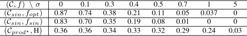
As argued at the beginning of this section, in a classical HO-DPA scenario, the evaluation process of a combining function must include an analysis in a noisy environment. Therefore, we analyzed the efficiency of the sine-based combining in the presence of noise. Namely, we added Gaussian noisesN1, N2∼
N(0, σ)to the Hamming weights in (31) and (33). We list in Table VIII the values of the correlation according to an increasing noise (withnequal to8).
TABLE VIII
CORRELATIONS FORCsinANDCprod?ACCORDING TOσ.
(C, f)\σ 0 0.1 0.3 0.4 0.5 0.7 1 5
(Csin, fopt) 0.87 0.74 0.38 0.21 0.11 0.05 0.037 0
(Csin, fsin) 0.83 0.70 0.35 0.19 0.08 0.01 0 0 Cprod?,H
0.36 0.36 0.34 0.33 0.32 0.29 0.24 0.03
It can be observed that the correlation for Csin quickly de-creases asσincreases. For a noise deviationσgreater or equal to
0.4(which is quite low) the product combining offers a greater correlation. This suggests that in a HO-DPA scenario (where the leakage is noisy), the sine-based combining function is not suitable.
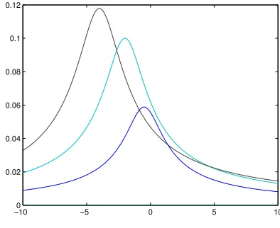
c) Final Comparison.: To conclude this section, Fig. 3 plots the correlations ρK with respect to the noise deviation σ∈[0,2]for the combining functions Csin,Cαprod? andCαdif f?, α∈ {1,2,3}. This plot underlines the previous conclusion: among the known combining functions, the improved product combining offers the best efficiency in a general leakage model.
V. CONCLUSION
In this paper, we have investigated higher order DPA at-tacks that combine several leakage signals to defeat masking countermeasures. We have first defined a theoretical framework allowing us to evaluate the efficiency of such an HO-DPA and we have shown how to optimize it according to the combining technique and the leakage model. This enabled us to study the existing combining techniques for second order DPA in the Hamming weight model with noise, paying particular attention to product combining and absolute difference combining. Our analysis allowed us to exhibit a way of significantly improving the product combining in this model and we showed that this improved product combining is more efficient than all the other techniques previously proposed in the literature.
0 0.5 1 1.5 2 0
0.1 0.2 0.3 0.4 0.5 0.6 0.7 0.8 0.9
Csin Cprod
Cdiff
Cdiff2 and Cdiff3 Cprod2 Cprod
3
Fig. 3. CorrelationρK for different combining functions according to the noise deviationσ.
Our work introduces the basis for a practically oriented analysis of HO-DPA attacks that may be used for future research. In particular, the framework proposed in this paper makes it possible to analyze the efficiency of new combining techniques in a general model. Moreover, our approach could be extended to the investigation HO-DPA of orders greater than two.
REFERENCES
[1] P. Kocher, J. Jaffe, and B. Jun, “Differential Power Analysis,” in
Advances in Cryptology – CRYPTO ’99, ser. Lecture Notes in Computer
Science, M. Wiener, Ed., vol. 1666. Springer, 1999, pp. 388–397. [2] S. Chari, J. Rao, and P. Rohatgi, “Template Attacks,” inCryptographic
Hardware and Embedded Systems – CHES 2002, ser. Lecture Notes in
Computer Science, B. Kaliski Jr., C¸ . Koc¸, and C. Paar, Eds., vol. 2523. Springer, 2002, pp. 13–29.
[3] W. Schindler, K. Lemke, and C. Paar, “A Stochastic Model for Dif-ferential Side Channel Cryptanalysis,” inCryptographic Hardware and
Embedded Systems – CHES 2005, ser. Lecture Notes in Computer
Science, J. Rao and B. Sunar, Eds., vol. 3659. Springer, 2005. [4] C. Archambeau, E. Peeters, F.-X. Standaert, and J.-J. Quisquater,
“Tem-plate Attacks in Principal Subspaces,” inCryptographic Hardware and
Embedded Systems – CHES 2006, ser. Lecture Notes in Computer
Science, L. Goubin and M. Matsui, Eds., vol. 4249. Springer, 2006, pp. 1–14.
[5] S. Chari, C. Jutla, J. Rao, and P. Rohatgi, “Towards Sound Approaches to Counteract Power-Analysis Attacks,” inAdvances in Cryptology –
CRYPTO ’99, ser. Lecture Notes in Computer Science, M. Wiener, Ed.,
vol. 1666. Springer, 1999, pp. 398–412.
[6] L. Goubin and J. Patarin, “DES and Differential Power Analysis – The Duplication Method,” inCryptographic Hardware and Embedded
Systems – CHES ’99, ser. Lecture Notes in Computer Science, C¸ . Koc¸
and C. Paar, Eds., vol. 1717. Springer, 1999, pp. 158–172.
[7] K. Schramm and C. Paar, “Higher Order Masking of the AES,” inTopics
in Cryptology – CT-RSA 2006, ser. Lecture Notes in Computer Science,
D. Pointcheval, Ed., vol. 3860. Springer, 2006, pp. 208–225. [8] J.-S. Coron, E. Prouff, and M. Rivain, “Side Channel Cryptanalysis of
a Higher Order Masking Scheme,” in Cryptographic Hardware and
Embedded Systems – CHES 2007, ser. Lecture Notes in Computer
Science, P. Paillier and I. Verbauwhede, Eds., vol. 4727. Springer, 2007, pp. 28–44.
[9] T. Messerges, “Securing the AES Finalists against Power Analysis Attacks,” inFast Software Encryption – FSE 2000, ser. Lecture Notes in Computer Science, B. Schneier, Ed., vol. 1978. Springer, 2000, pp. 150–164.
[10] M.-L. Akkar and C. Giraud, “An Implementation of DES and AES, Secure against Some Attacks,” inCryptographic Hardware and
C¸ . Koc¸, D. Naccache, and C. Paar, Eds., vol. 2162. Springer, 2001, pp. 309–318.
[11] T. Messerges, “Using Second-order Power Analysis to Attack DPA Resistant Software,” inCryptographic Hardware and Embedded Systems
– CHES 2000, ser. Lecture Notes in Computer Science, C¸ . Koc¸ and
C. Paar, Eds., vol. 1965. Springer, 2000, pp. 238–251.
[12] J. Waddle and D. Wagner, “Toward Efficient Second-order Power Analy-sis,” inCryptographic Hardware and Embedded Systems – CHES 2004, ser. Lecture Notes in Computer Science, M. Joye and J.-J. Quisquater, Eds., vol. 3156. Springer, 2004, pp. 1–15.
[13] M. Joye, P. Paillier, and B. Schoenmakers, “On Second-order Differential Power Analysis,” inCryptographic Hardware and Embedded Systems
– CHES 2005, ser. Lecture Notes in Computer Science, J. Rao and
B. Sunar, Eds., vol. 3659. Springer, 2005, pp. 293–308.
[14] E. Peeters, F.-X. Standaert, N. Donckers, and J.-J. Quisquater, “Im-proved Higher-order Side-Channel Attacks with FPGA Experiments,”
inCryptographic Hardware and Embedded Systems – CHES 2005, ser.
Lecture Notes in Computer Science, J. Rao and B. Sunar, Eds., vol. 3659. Springer, 2005, pp. 309–323.
[15] F.-X. Standaert, E. Peeters, and J.-J. Quisquater, “On the Masking Coun-termeasure and Higher Order Power Analysis Attacks,” inITCC ’05: Proceedings of the International Conference on Information Technology:
Coding and Computing (ITCC’05) - Volume I. IEEE Computer Society,
2005, pp. 562–567.
[16] E. Oswald, S. Mangard, C. Herbst, and S. Tillich, “Practical Second-order DPA Attacks for Masked Smart Card Implementations of Block Ciphers,” inTopics in Cryptology – CT-RSA 2006, ser. Lecture Notes in Computer Science, D. Pointcheval, Ed., vol. 3860. Springer, 2006, pp. 192–207.
[17] E. Brier, C. Clavier, and F. Olivier, “Correlation Power Analysis with a Leakage Model,” inCryptographic Hardware and Embedded Systems –
CHES 2004, ser. Lecture Notes in Computer Science, M. Joye and J.-J.
Quisquater, Eds., vol. 3156. Springer, 2004, pp. 16–29.
[18] S. Mangard, “Hardware Countermeasures against DPA – A Statistical Analysis of Their Effectiveness,” in Topics in Cryptology – CT-RSA 2004, ser. Lecture Notes in Computer Science, T. Okamoto, Ed., vol. 2964. Springer, 2004, pp. 222–235.
[19] S. Mangard, E. Oswald, and T. Popp,Power Analysis Attacks – Revealing
the Secrets of Smartcards. Springer, 2007.
[20] F.-X. Standaert, E. Peeters, G. Rouvroy, and J.-J. Quisquater, “An Overview of Power Analysis Attacks Against Field Programmable Gate Arrays,”IEEE, vol. 94, no. 2, pp. 383–394, 2006.
[21] E. Oswald and S. Mangard, “Template Attacks on Masking—Resistance is Futile,” inTopics in Cryptology – CT-RSA 2007, ser. Lecture Notes in Computer Science, M. Abe, Ed., vol. 4377. Springer, 2007, pp. 243–256.
[22] M. Joye and J.-J. Quisquater, Eds.,Cryptographic Hardware and
Em-bedded Systems – CHES 2004, ser. Lecture Notes in Computer Science,
vol. 3156. Springer, 2004.
[23] M. Wiener, Ed.,Advances in Cryptology – CRYPTO ’99, ser. Lecture Notes in Computer Science, vol. 1666. Springer, 1999.
[24] J. Rao and B. Sunar, Eds., Cryptographic Hardware and Embedded
Systems – CHES 2005, ser. Lecture Notes in Computer Science, vol.
3659. Springer, 2005.
[25] D. Pointcheval, Ed.,Topics in Cryptology – CT-RSA 2006, ser. Lecture Notes in Computer Science, vol. 3860. Springer, 2006.
APPENDIXI USEFULLEMMAS
Lemma 20: Letnbe a positive integer and letM be a random variable uniformly distributed overFn2. Then, we have:
EhH(M)2i= n
2
+n
4 (34)
Proof: SinceM is uniformly distributed over Fn2, we have
EhH(M)2i=E
n
X
i,j=1
M[i]M[j]
,
that is
EhH(M)2i=
n
X
i,j=1 i6=j
E[M[i]M[j]] +
n
X
i=1
E[M[i]] ,
For every i6=j, we have E[M[i]M[j]] = 14 and E[M[i]] = 12. Hence we deduce EhH(M)2
i
=n(n−1)×14+n×12 =n24+n. Lemma 21: Letnbe a positive integer and letMbe a random variable uniformly distributed overFn2. Then, for everyz ∈Fn2, we have:
E[H(z⊕M)H(M)] =−1
2H(z) +
n2+n
4 . (35)
Proof: From Property 2 we have
E[H(z⊕M)H(M)] =H(z)E[H(M)] +EhH(M)2i
−2E[H(z∧M)H(M)] . (36) SinceM is uniformly distributed, we have E[H(M)] = n2 and EhH(M)2i = n24+n (from Lemma 20). On the other hand, E[H(z∧M)H(M)] satisfies
E[H(z∧M)H(M)] =
n
X
i=0
z[i]E[M[i]H(M)] . (37)
SinceM is uniformly distributed overFn2, E[M[i]H(M)]is equal ton1EhH(M)2ii.e.ton+14 (from Lemma 20). Hence simplifying (36) leads to (35).
Lemma 22: Letmandnbe two integers and letrbe a positive integer:
X
k r m+k
!
s n+k
!
= r+s
r−m+n
!
. (38)
Proof: Lemma 22 is a well-known result whose proof can be found in [?].
APPENDIXII
PROOFS OFPROPOSITIONS14AND16
A. Proof of Proposition 14
Proof: For every pair(z, m)∈Fn2, Property 2 implies|H(z⊕ m)−H(m)|=|H(z)−2H(z∧m)|from which we deduce:
E[|H(z⊕M)−H(M)|] = H(z)
X
i=0
|H(z)−2i|P[H(z∧M) =i] . (39) Since M is uniformly distributed P[H(z∧M) =i] equals
2−H(z) H(iz)
. Hence we deduce
E[|H(z⊕M)−H(M)|] = 2−H(z)
bH(z) 2 c
X
i=0 H(z)
i
!
(H(z)−2i) . (40)
By symmetry, we have Pb
H(z) 2 c i=0
H(z) i
equal to
1 2
PH(z)
i=0
H(z) i
+ HH((zz))
2
(H(z) mod 2)
. Then P
i
H(z) i
=
2H(z)implies
bH(z) 2 c
X
i=0 H(z)
i
!
=
2H(z)−1+1 2
H(z) H(z) 2
!
On the other hand H(iz)
iequals H(z) H(iz−)−11which in a similar way gives
bH(2z)c X
i=0 H(z)
i
!
i=H(z)
2 2
H(z)−1
−H(z)
2
H(z)−1 H(z)−1
2
!
×(H(z) mod 2) . (42) Finally, (40), (41) and (42) lead to (25)
B. Proof of Proposition 16
Proof: Let φB and ΦB respectively denote the proba-bility density function and the probaproba-bility distribution function of B (that is ΦB(y) = P[B≤y] =
Ry
−∞φB(x) dx). As B has a gaussian distribution N(0, σ0), we have φB(x) =
1 √
2πσ0
exp(−x2/2σ02). Then we have: E[|s+B|] =
Z+∞ −∞
|s+x|φB(x) dx
= s
Z s −s
φB(x)dx +
Z s −s
xφB(x)dx
+2 Z +∞
s
xφB(x)dx .
Since the functionx7→xφB(x)is odd, the term
Rs
−sxφB(x) dx equals zero. Moreover, we haveRs
−sφB(x)dx= 2 ΦB(s)− 1 2
andR+∞
s xφB(x)dx=√σ20πexp
−s2/2σ20. Hence, we get E[|s+B|] = 2s
ΦB(s)−
1 2
+
√
2σ0
√
π exp
−s2/2σ20
. (43)
Finally, since B has a gaussian distribution N(0, σ0), its probability distribution function ΦB satisfies ΦB(y) =
1 2
1 +erf√y 2σ0
for everyy∈Rhence (43) directly implies