A Dependent Multilabel Classification Method Derived from the k-Nearest Neighbor Rule

Volume 2011, Article ID 645964,14pages doi:10.1155/2011/645964

Research Article

A Dependent Multilabel Classification Method Derived from

the

k

-Nearest Neighbor Rule

Zoulficar Younes (EURASIP Member),

1

_{Fahed Abdallah,}

1

Thierry Denoeux,

1

_{and Hichem Snoussi}

2

1_{Heudiasyc, UMR CNRS 6599, University of Technology of Compi`egne, 60205 Compi`egne, France}

2_{ICD-LM2S, FRE CNRS 2848, University of Technology of Troyes, 10010 Troyes, France}

Correspondence should be addressed to Zoulficar Younes,[email protected]

Received 17 June 2010; Revised 9 January 2011; Accepted 21 February 2011

Academic Editor: B¨ulent Sankur

Copyright © 2011 Zoulficar Younes et al. This is an open access article distributed under the Creative Commons Attribution License, which permits unrestricted use, distribution, and reproduction in any medium, provided the original work is properly cited.

In multilabel classification, each instance in the training set is associated with a set of labels, and the task is to output a label set whose size is unknowna priorifor each unseen instance. The most commonly used approach for multilabel classification is where a binary classifier is learned independently for each possible class. However, multilabeled data generally exhibit relationships between labels, and this approach fails to take such relationships into account. In this paper, we describe an original method for multilabel classification problems derived from a Bayesian version of thek-nearest neighbor (k-NN) rule. The method developed here is an improvement on an existing method for multilabel classification, namely multilabelk-NN, which takes into account the dependencies between labels. Experiments on simulated and benchmark datasets show the usefulness and the efficiency of the proposed approach as compared to other existing methods.

1. Introduction

Traditional single-label classification assigns an object to exactly one class, from a set ofQdisjoint classes.Multilabel classification is the task of assigning an instance simulta-neously to one or multiple classes. In other words, the target classes are not exclusive: an object may belong to an unrestricted set of classes, rather than to exactly one class. For multilabeled data, an instance may belong to more than one class not because of ambiguity (fuzzy membership), but because of multiplicity (full membership) [1]. Note that traditional supervised learning problems (binary or multi-class) can be regarded as special cases of the problem of multilabel learning, where instances are restricted to belonging to a single class.

Recently, multilabel classification methods have been increasingly required by modern applications where it is quite natural for some instances to belong to several classes at once. Typical examples of multilabel problems are text cat-egorization, functional genomics, and scene classification. In text categorization, each document may belong to multiple

topics, such asartsandhumanities[2–5]; in gene functional analysis, each gene may be associated with a set of functional classes, such as energy, metabolism, and cellular biogenesis

[6]; in natural scene classification, each image may belong to several image types at the same time, such asseaandsunset

[1].

A common approach to a multilabel learning problem is to transform it into one or more single-label problems. The best known transformation method is thebinary relevance

(BR) approach [7]. This approach transforms a multilabel classification problem withQpossible classes intoQ single-label classification problems. Theqth single-label classifica-tion problem (q ∈ {1,. . .,Q}) consists in separating the instances belonging to classωqfrom the others. This problem

is solved by training a binary classifier (0/1 decision) where each instance in the training set is considered to bepositive

if it belongs to ωq, andnegative otherwise. The output of

independently: when one label provides information about another, the binary classifier fails to capture this effect. For example, if a news article belongs to a “music” category, it is very likely that it also belongs to an “entertainment” category. Although the BR approach is generally criticized for its assumption of label independencies [8, 9], it is a simple, intuitive approach that has the advantage of having low computational complexity.

In [10], the authors present a Bayesian multilabel k -nearest neighbor (MLkNN) approach where, in order to assign a set of labels to a new instance, a decision is made separately for each label by taking into account the number of neighbors containing the label to be assigned. This method therefore fails to take into account the dependency between labels.

In this paper, we present a generalization of the MLk NN-based approach to multilabel classification problems where the dependencies between classes are considered. We call this method DMLkNN, for dependent multilabelk-nearest Neighbor. The principle of the method is as follows. For each unseen instance, we identify its k-NNs in the training set. According to the class membership of neighboring instances, aglobal maximum a posteriori (MAP) principle is used in order to assign a set of labels to the new unseen instance. Note that unlike MLkNN, in order to decide whether a particular label should be included among the unseen instance’s labels, the global MAP rule takes into account the numbers of different labels in the neighborhood, instead of considering only the number of neighbors having the label in question.

Note that this paper is an extension of a previously published conference paper [11]. Here, the method is more thoroughly interpreted and discussed. Extensive compar-isons on several real world datasets and with some state-of-the-art methods are added in the experimental section. In addition, we provide an illustrative example on a simulated dataset, where we explain step by step the principle of our algorithm.

The remainder of the paper is organized as follows.

Section 2 presents related work. Section 3 describes the principle of multilabel classification and the notion of label dependencies. Section 4 introduces the DMLkNN method and its implementation. Section 5 presents some experiments and discusses the results. Finally, Section 6

summarizes this work and makes concluding remarks.

2. Related Work

Several methods have been proposed in the literature for multilabel learning. These methods can be categorized into two groups. A first group contains theindirectmethods that transform a multilabel classification problem into binary classification problems (a binary classifier for each class or pairwise classifiers) [1,9] or into multi-class classification problem (each subset of classes is considered as a new class) [7]. A second group consists in extending common learning algorithms and making them able to manipulate multilabel datadirectly[12]. Some multilabel classification methods are briefly described below.

In [13], an adaptation of the traditional radial basis function (RBF) neural network for multilabel learning is presented. It consists of two layers of neurons: a first layer of hidden neurons representing basis functions associated with prototype vectors, and a second layer of output neurons related to all possible classes. The proposed method, named MLRBF, first performs a clustering of the instances corresponding to each possible class; the prototype vectors of the first-layer basis functions are then set to the centroids of the clustered groups. In a second step, the weights of the second-layer are fixed by minimizing a sum-of-squares error function. The output neuron of each class is connected to all input neurons corresponding to the prototype vectors of the different possible classes. Therefore, information encoded in the prototype vectors of all classes is fully exploited when optimizing the connection weights and predicting the label sets for unseen instances.

In [6], a multilabel ranking approach based on support vector machines (SVM) is presented. The authors define a cost function and a special multilabel margin and then propose an algorithm named RankSVM based on a ranking system combined with a label set size predictor. The set size predictor is computed from a threshold value that separates the relevant from the irrelevant labels. The value is chosen by solving a learning problem. The goal is to minimize a ranking loss function while having a large margin. RankSVM uses kernels rather than linear dot products, and the optimization problem is solved via its dual transformation.

In [12], an evidence-theoretick-NN rule for multilabel classification is presented. This rule is based on an evidential formalism for representing uncertainties in the classification of multilabeled data and handling imprecise labels, described in detail in [14]. The formalism extends all the notions of Dempster-Shafer theory [15] to the multilabel case, with only a moderate increase in complexity as compared to the classical case. Under this formalism, each piece of evidence about an instance to be classified is represented by a pair of sets: a set of classes that surely apply to the unseen instance, and a set of classes that surely do not apply to this instance.

A distinction should be made between multilabel and

multiple-label learning problems. Multiple-label learning [16] is a semisupervised learning problem for single-label classification where each instance is associated with a set of labels, but where only one of the candidate labels is the true label for the given instance. For example, this situation occurs when the training data is labeled by several experts and, owing to conflicts and disagreements between the experts, a set of labels, rather than exactly one label, is assigned to some instances. The set of labels of an instance contains the decision (the assigned label) made by each expert about this instance. This means that there is an ambiguity in the class labels of the training instances.

Another learning problem is multi-instance multilabel

the document in question, while the document may deal with several topics at the same time, such ascultureandsociety.

In [18],dynamic conditional random fields(DCRFs) are presented for representing and handling complex interac-tion between labels in sequence modeling, such as when performing multiple, cascaded labeling tasks on the same sequence. DCRFs are a generalization of conditional random fields. Inference in DCRFs can be done using approximate methods, and training can be done by maximuma posteriori

estimation.

3. Multilabel Classification

3.1. Principle. LetX = Rd _{denote the domain of instances}

and let Y = {ω1,ω2,. . .,ωQ} be the finite set of labels.

The multilabel classification problem can be formulated as follows. Given a setD = {(x1,Y1), (x2,Y2),. . ., (xn,Yn)}of ntraining examples, independently drawn fromX×2Y, and identically distributed, wherexi ∈XandYi ⊆Y, the goal

of the learning system is to build a multilabel classifierH :

X →2Yin order to assign a label set to each unseen instance. As for standard classification problems, we can associate with the multilabel classifierH a scoring function f : X×

Y → R, which assigns a real number to each instance/label combination (x,ω)∈X×Y. The scoref(x,ω) corresponds to the probability that instance xbelongs to classω. Given any instancexwith its known set of labelsY⊆Y, the scoring functionf is assumed to give larger scores for labels inYthan it does for those not inY. In other words,f(x,ωq)> f(x,ωr)

for anyωq ∈Y andωr ∈/ Y. The scoring function f allows

us to rank the different labels according to their scores. For an instance x, the higher the rank of a label ω, the larger the value of the corresponding score f(x,ω). Note that the multilabel classifierH(·) can be derived from the function

f(·,·) via thresholding:

H(x)=ω∈Y| f(x,ω)≥t, (1)

wheretis a threshold value.

3.2. Label Dependencies in Multilabel Applications. In multi-label classification, the assignment of classωto an instancex

may provide information about that instance’s membership of other classes. Label dependencies exist when the prob-ability of an instance belonging to a class depends on its membership of other classes. For example, a document with the topic politicsis unlikely to be labeled asentertainment, but the probability that the document belongs to the class

economicis high.

In general, relationships between labels are high order or even full order, that is, there is a relation between a label and all remaining labels, but these relations are more difficult to represent than second-order relations, that is, relations that exist between pairs of labels. The dependencies between labels can be represented in the form of a contingency matrix mat that allows us to express only second-order relations between labels. Let Hq1 denote the hypothesis that instance xbelongs to classωq ∈ Y. Given a multilabeled datasetD

with Qpossible labels, mat[q] [r] = Pr(Hq1 | Hr1), where

6 4 5 3 2 1

1 2 3 4 5 6 0

0.1 0.2 0.3 0.4 0.5 0.6 0.7

Figure1: Contingency matrix for the emotion dataset.

q and r ∈ {1,. . .,Q} with q /=r, indicates the second-order relationship between labels ωq and ωr. Pr(Hq1 | Hr1)

represents the proportion of data in D belonging to ωr

to which label ωq is also assigned. mat[q] [q] = Pr(Hq1)

indicates the frequency of labelωqin the datasetD.Figure 1

shows the contingency matrix for the emotion dataset (Q=

6) used in the experiments inSection 5. In this dataset, each instance represents a song and is labeled by the emotions evoked by this song. We can see inFigure 1that mat[1] [4]=

Pr(H1₁ | H4₁) = 0, meaning that labels ω1 and ω4 cannot

occur together. This is easily interpretable, asω1corresponds

to “amazed-surprised” whileω4corresponds to “quiet-still”,

and these two emotions are clearly opposite. We can also see that mat[5] [4] = Pr(H5₁ | H4₁) = 0.6, which means that

ω5, representing “sad-lonely”, frequently coexists in the label

sets withω4. We can deduce from these examples that labels

in multilabeled datasets are often mutually dependent, and exploiting relationships between labels will be very helpful in improving classification performance.

4. The DMLkNN Method for

Multilabel Classification

We use the same notation as in [10] in order to facilitate comparison with the MLkNN method. Given an instancex

and its associated label setY ⊆ Y, letNk

x denote the set of

thek closest training examples ofx in the training dataset

Daccording to a distance function d(·,·), and letyxbe the Q-dimensional categoryvector ofx whose qth component indicates whetherxbelongs to classωq:

yx

q=

⎧ ⎨ ⎩

1, ifωq∈Y,

0, otherwise, ∀q∈ {1,. . .,Q}. (2)

Let us represent by cx the Q-dimensional membership

counting vector ofx, theqth component of which indicates how many examples amongst thek-NNs ofxbelong to class

ωq:

cx

q= xi∈Nxk

yxi

4.1. MAP Principle. Let x now denote an instance to be classified. Like in allk-NN based methods, when classifying a test instance x, the set Nk

x of its k nearest neighbors

should first be identified. Under the multilabel assumption, the counting vector cx is computed. As mentioned before,

let Hq1denote the hypothesis thatxbelongs to classωq, and

Hq₀ the hypothesis thatx should not be assigned toωq. Let

Eqj (j ∈ {0, 1,. . .,k}) denote the event that there are exactly j instances inNk

x belonging to classωq. To determine the qth component of the category vectoryx for instancex, the

MLkNN algorithm uses the following MAP [10]:

yx

q=arg max

b∈{0,1}

Pr

Hq_b|Eq_c

x(q)

, (4)

while for the DMLkNN algorithm, the following MAP is used:

yx

q=arg max

b∈{0,1}

Pr

⎛ ⎝_Hq

b|

ωl∈Y

Elcx(l)

⎞ ⎠

=arg max

b∈{0,1}

Pr

⎛ ⎝_Hq

b|E q cx(q),

ωl∈Y\{ωq}

El_cx(l)

⎞ ⎠_.

(5)

In contrast to decision rule (4), we can see from (5) that the assignment of labelωqto the test instancexdepends not only

on the event that there are exactlycx(q) instances having label ωqinNxk, that is, E

q

cx(q), but also on

ωl∈Y\{ωq}E l

cx(l), which is

the event that there are exactlycx(l) instances having label ωl in Nxk, for each ωl ∈ Y\ {ωq}. Thus, it is clear that

label correlation is taken into account in (5), since all the components of the counting vector cx are involved in the

assignment or not of labelωqtox, which is not the case in

(4).

4.2. Posterior Probability Estimation. Regarding the counting vectorcx, the number of possible events

ωl∈YE l

cx(l)is upper

bounded by (k+ 1)Q. This means that, in addition to the complexity problem, the estimation of (5) from a relatively small training set will not be accurate. To overcome this difficulty, we will adopt a fuzzy approximation for (5). This approximation is based on the event Fl_j, j ∈ {0, 1,. . .,k}, which is the event that there are approximately j instances inNk

x belonging to classωl, that is, Flj, denotes the event that

the number of instances inNk

x that are assigned labelωlis in

the interval [j−δ;j+δ], whereδ∈ {0,. . .,k}is afuzziness

parameter. As a consequence, we can derive a fuzzy MAP rule

yx

q=arg max

b∈{0,1}

Pr

⎛ ⎝_Hq

b|

ωl∈Y

Flcx(l)

⎞

⎠_{. (6)}

To remain closer to the initial formulation and for compari-son with MLkNN, (6) will be replaced by the following rule:

yx

q=arg max

b∈{0,1}

Pr

⎛ ⎝_Hq

b|E q cx(q),

ωl∈Y\{ωq}

Fl_cx(l)

⎞ ⎠_{. (7)}

For large values of δ, the results of our method will be similar to those of MLkNN. In fact, forδ =k, the MLkNN algorithm is a particular case of the DMLkNN algorithm, whereωl∈Y\{ωq}F

l

cx(l)will becertain, because for eachωl ∈

Y\ {ωq}, the number of instances inNxkbelonging to class ωlwill surely be in the interval [j−k;j+k]. For small values

of δ, the assignment or not of labelωq to test instance x

will not only depend on the number of instances inNk x that

belong to labelωq, but also on the number of instances inNxk

belonging to the remaining labels.

Using Bayes’ rule, (4) and (7) can be written as follows:

yx

q=arg max

b∈{0,1}

PrHq_bPr

Eq_c

x(q)|H

q b

Pr

Eq_c

x(q)

=arg max

b∈{0,1}

PrHq_bPr

Eq_c

x(q)|H

q b . (8) yx

q=arg max

b∈{0,1}

PrHq_bPr

Eq_c

x(q),

ωl∈Y\{ωq}F l cx(l)|H

q b

Pr

Eq_c

x(q),

ωl∈Y\{ωq}F l cx(l)

=arg max

b∈{0,1}

PrHq_bPr

⎛ ⎝Eq

cx(q),

ωl∈Y\{ωq}

Fl cx(l)|H

q b

⎞ ⎠.

(9)

To rank labels inY, aQ-dimensional real-valued vector

rxcan be calculated. Theqth component ofrxis defined as

the posterior probability Pr(Hq1|E q cx(q),

ωl∈Y\{ωq}F l cx(l))

rx

q=Pr

⎛ ⎝_Hq

1|E

q cx(q),

ωl∈Y\{ωq}

Fl_cx(l)

⎞ ⎠

=Pr

Hq1

Pr

Eq_c

x(q),

ωl∈Y\{ωq}F l cx(l)|H

q 1

Pr

Eq_c

x(q),

ωl∈Y\{ωq}F l cx(l)

=

PrHq1

Pr

Eq_c

x(q),

ωl∈Y\{ωq}F l cx(l)|H

q 1

b∈{0,1}Pr

Hq_bPr

Eq_c

x(q),

ωl∈Y\{ωq}F l cx(l)|H

q b

.

(10)

For comparison, the real-valued vectorrx for MLkNN has

the following expression:

r_xq=Pr

Hq₁|Eq_c

x(q)

=

PrHq1

Pr

Eq_c

x(q)|H

q 1 Pr Eq

cx(q)

=

PrHq₁Pr

Eq

cx(q)|H

q 1

b∈{0,1}Pr

Hq_bPr

Eq_c

x(q)|H

q b

.

[yx,rx]=DMLkNN(D,x,k,s,δ)

%Computing the prior probabilities and the number of instances belonging to each class (1) Forq=1,. . .,Q

(2) Pr(Hq1)=(

m

i=1yxi(q))/(n); Pr(H q

0)=1−Pr(H

q

1);

(3) u(q)=n

i=1yxi(q);u(q)=n−u(q); EndFor

%For each test instancex

(4) IdentifyN(x) andcx

%Counting the training instances whose membership counting vectors satisfy the constraints (15) (5) Forq=1,. . .,Q

(6) v(q)=0;v(q)=0 EndFor

(7) Fori=1,. . .,n

(8) IdentifyN(xi) andcxi

(9) If cx(q)−δ≤cxi(q)≤cx(q) +δ,∀q∈YThen

(10) Forq=1,. . .,Q

(11) If cxi(q)==cx(q)Then

(12) If yxi(q)==1Then v(q)=v(q) + 1;

Else v_{(q)=v(q) + 1;}

EndFor EndFor

%Computingyxandrx (13) Forq=1,. . .,Q (14) Pr(Eqcx(q),

ωl∈Y\{ωq}F l cx(l)|H

q

1)=(s+v(q))/(s×Q+u(q));

(15) Pr(Eqcx(q),

ωl∈Y\{ωq}F l cx(l)|H

q

0)=(s+v(q))/(s×Q+u(q));

(16) yx(q)=arg maxb∈{0,1}Pr(Hqb)Pr(E q cx(q),

ωl∈Y\{ωq}F l cx(l)|H

q b)

(17) rx(q)= Pr(H q

1)Pr(E

q cx(q),

ωl∈Y\{ωq}F l cx(l)|H

q

1)

b∈{0,1}Pr(Hqb)Pr(E q cx(q),

ωl∈Y\{ωq}F l cx(l)|H

q b) EndFor

Algorithm1: DMLkNN algorithm.

In order to determine the category vector yx and the

real-valued vector rx of instance x, we need to

deter-mine the prior probabilities Pr(Hl

b) and the likelihoods

Pr(Eqcx(q),

ωl∈Y\{ωq}F l cx(l)|H

q

b), for eachq∈ {1,. . .,Q}, and b∈ {0, 1}. These probabilities are estimated from a training datasetD.

Given an instance x to be classified, the output of the DMLkNN method for multilabel classification is determined as follows:

H(x)=ωq∈Y|yx

q=1,

fx,ωq

=rx

q, for eachωq∈Y.

(12)

Algorithm 1 shows the pseudocode of the DMLkNN algorithm. The value of δ may be selected through cross-validation and provided as input to the algorithm. The prior probabilities Pr(Hq_b),b = {0, 1}, for each classωq are first

calculated and the instances belonging to each label are counted (steps (1) to (3)):

PrHq1

= 1

n n

i=1 yxi

q,

PrHq₀=1−PrHq₁.

(13)

Recall that n is the number of training instances. u(q) is the number of instances belonging to class ωq, and u(q)

indicates the number of instances not havingωqin their label

sets:

uq=

n

i=1 yxi

q,

uq=n−uq.

(14)

For test instance x, the k-NNs are identified and the membership counting vector cx is determined (step (4)).

To decide whether or not to assign the label ωq to x, we

must determine the likelihoods Pr(Eq_cx(q),ωl∈Y\{ωq}F l cx(l) |

Hq_b), b ∈ {0, 1}, using the training instances such that their corresponding membership counting vectors satisfy the following constraints:

cxi

q=cx

q,

cx(l)−δ≤cxi(l)≤cx(l) +δ, for eachωl∈Y\

ωq

.

(15)

1 2

1 2

1

1 2 2

1

1 2 3 1

1 3

1

(a)

1 2

1

1

1 2 2

1

1 23 1

1 3

1

(b)

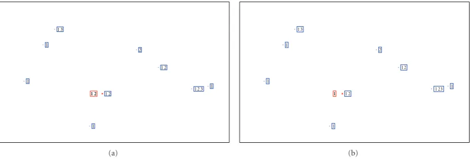
Figure2: Estimated label set (in bold) for a test instance using the DMLkNN (a) and MLkNN (b) methods.

remaining instances satisfying the previous constraints and not havingωq in their sets of labels is stored inv(q). The

likelihoods Pr(Eq_cx(q),ωl∈Y\{ωq}F l cx(l) | H

q

b), b ∈ {0, 1}, are

then computed

Pr

⎛ ⎝_Eq

cx(q),

ωl∈Y\{ωq}

Fl_cx(l)|Hq1

⎞

⎠₌ s+v(l)

s×Q+u(l),

Pr

⎛ ⎝Eq

cx(q),

ωl∈Y\{ωq}

Fl cx(l)|H

q 0

⎞

⎠₌ s+v(l)

s×Q+u_(l),

(16)

where s is a smoothing parameter [19]. Smoothing is commonly used to avoid zero probability estimates. When

s = 1, it is called Laplace smoothing. Finally, the category vectoryx and the real-valued vectorrx to rank labels inY

are calculated using (9) and (10), respectively (steps (13) to (17)).

Note that, in the MLkNN algorithm, only the first con-straint in (15) is considered when computing the likelihoods Pr(Eq_cx(q) | Hq_b), b ∈ {0, 1}. As a result, the number of examples in the learning set satisfying this constraint is larger than the number of examples satisfying (15). MLkNN and DMLkNN should therefore not necessarily be compared using the same smoothing parameter.

4.3. Illustration on a Simulated Dataset. In this subsection, we illustrate the behavior of the DMLkNN and MLkNN methods using simulated data.

The simulated dataset contains 1019 instances in R2

belonging to three possible classes, Y = {ω1,ω2,ω3}.

The data were generated from seven Gaussian distribu-tions with means (0, 0), (1, 0), (0.5, 0), (0.5, 1), (0.25, 0.6), (0.75, 0.6), (0.5, 0.5), respectively, and equal covariance matrix 1 00 1

. The number of instances in each class is chosen arbitrarily (see Table 1). Taking into account the geometric distribution of the Gaussian data, the instances of each set were, respectively, assigned to label(s)

{ω1},{ω2},{ω1,ω2},{ω3},{ω1,ω3},{ω2,ω3},{ω1,ω2,ω3}.

Figure 2 shows the neighboring training instances and the estimated label set for a test instancexusing DMLkNN and MLkNN. For both methods,kwas set to 8, and Laplace

smoothing (s =1) was used. For DMLkNN,δwas set to 1. Below we describe the different steps in the estimation of the label set ofxusing the DMLkNN and MLkNN algorithms applied to the test data. For the sake of clarity we recall some definitions of events already given above. The membership counting vector of the test instance iscx=(7, 3, 2). Using the

DMLkNN method, in order to estimate the label set ofx, the following probabilities need to be computed from (9):

yx(1)=arg max b∈{0,1}

PrH1_bPrE1₇, F2₃, F3₂|H1_b,

yx(2)=arg max b∈{0,1}

PrH2_bPrE2₃, F1₇, F3₂|H2_b,

yx(3)=arg max b∈{0,1}

PrH3_bPrE3₂, F1₇, F2₃|H3_b.

(17)

We recall that E17is the event that there are seven instances in

Nk

x which have labelω1, and F23is the event that the number

of instances inNk

x belonging to labelω2is in the interval [3− δ; 3 +δ]=[2, 4]. In contrast, for estimating the label set of the unseen instance using the MLkNN method, the following probabilities must be computed from (8):

y_x(1)=arg max

b∈{0,1}

PrH1_bPrE1₇|H1_b,

y_x(2)=arg max

b∈{0,1}

PrH2_bPrE2₃|H2_b,

y_x(3)=arg max

b∈{0,1}

PrH3_bPrE3₂|H3_b.

(18)

First, the prior probabilities are computed from the training set according to (13):

PrH11

=0.4527, PrH10

=0.5473,

PrH2 1

=0.5038, PrH2 0

=0.4962,

PrH3₁=0.4396, PrH3₀=0.5604.

(19)

DMLkNN, this is done according to steps (7) to (15), as shown inAlgorithm 1and explained inSection 4.2.)

PrE17, F23, F32|H11

=0.0478, PrE17, F23, F32|H10

=0.0139,

PrE2₃, F1₇, F₂3|H2₁=0.0237, PrE2₃, F1₇, F₂3|H2₀=0.0218,

PrE32, F17, F23|H31

=0.0394, PrE32, F17, F23|H30

=0.1161,

PrE1₇|H1₁=0.1108, PrE1₇|H1₀=0.0431,

PrE23|H21

=0.1231, PrE23|H20

=0.1746,

PrE32|H31

=0.0655, PrE32|H30

=0.0593.

(20)

Using the prior and the posterior probabilities, the category vectors associated to the test instance by the DMLkNN and MLkNN algorithms can be calculated

yx(1)=1, yx(1)=1,

yx(2)=1, yx(2)=0,

yx(3)=0, yx(3)=0.

(21)

Thus, the estimated label set for instancexgiven by the DMLkNN method is Y = {ω1,ω2}, while that given by

MLkNN is Y = {ω1}. The true label set for x is Y =

{ω1,ω2}. Here, we can see that no error has occurred when

estimating the label set of x using the DMLkNN method, while for MLkNN the estimated label set is not identical to the ground truth label set. Seven training instances in Nk

x have class ω1 in their label sets, while only three

instances belong to ω2. In fact, the existence of classω1 in

the neighborhood of x gives some information about the existence or not of class ω2 in the label set ofx. If we take

a look at the training dataset, we remark that 14.7% of instances belong toω1, 15.9% toω2, and 29.8% toω1 and ω2 simultaneously. Thus, the probability that an instance

belongs to both classesω1andω2is approximately twice the

probability that it belongs to only one of the two classes. DMLkNN is able to capture the relationship between classes

ω1andω2, while MLkNN is not able to capture this relation.

This example shows that the DMLkNN method, which takes into account the dependencies between labels, may improve the classification performance and estimate the label sets of test instances with greater accuracy.

5. Experiments

In this section, we report a comparative study between DMLkNN and some state-of-the-art methods on several datasets collected from real world applications, and using different evaluation metrics.

5.1. Evaluation Metrics. There exist a number of evaluation criteria that evaluate the performance of a multilabel learn-ing system, given a setD = {(x1,Y1),. . ., (xn,Yn)}ofntest

Table1: Summary of the simulated data set.

Label set Number of instances

{ω1} 150

{ω2} 162

{ω1,ω2} 304

{ω3} 262

{ω1,ω3} 43

{ω2,ω3} 78

{ω1,ω2,ω3} 20

examples. We now describe some of the main evaluation criteria used in the literature to evaluate a multilabel learning system [3,7]. The evaluation metrics can be divided into two groups: prediction-based and ranking-based metrics. Prediction-based metrics assess the correctness of the label sets predicted by the multilabel classifierH, while ranking-based metrics evaluate the label ranking quality depending on the scoring function f. Since not all multilabel classifica-tion methods compute a scoring funcclassifica-tion, predicclassifica-tion-based metrics are of more general use.

5.1.1. Prediction-Based Metrics

Accuracy. The accuracy metric is an average degree of similarity between the predicted and the ground truth label sets of all test examples:

Acc (H,D)=1 n

n

i=1

Yi∩Yi

Yi∪Yi

, (22)

whereYi=H(xi) denotes the predicted label set of instance xi.

F1-Measure. The F1-measure is defined as the harmonic mean of two other metrics known as precision (Prec) and recall (Rec) [20]. The former computes the proportion of correct positive predictions while the latter calculates the proportion of true labels that have been predicted as positives. These metrics are defined as follows:

Prec (H,D)= 1 n

n

i=1

Yi∩Yi

_Y

i

,

Rec (H,D)= 1 n

n

i=1

Yi∩Yi

|Yi| ,

F1(H,D)=2·Prec·Rec

Prec + Rec = 1

n n

i=1

2Yi∩Yi

|Yi|+Yi .

(23)

Hamming Loss. This metric counts prediction errors (an incorrect label is predicted) and missing errors (a true label is not predicted)

HLoss (H,D)= 1 n

n

i=1

1

Q

Table2: Characteristics of datasets.

Dataset Domain Number of instances Feature vector dimension Number of labels Label cardinality Label density Distinct label sets

Emotion Music 593 72 6 1.868 0.311 27

Scene Image 2407 294 6 1.074 0.179 15

Yeast Biology 2417 103 14 4.237 0.303 198

Medical Text 978 1449 45 1.245 0.028 94

Enron Text 1702 1001 53 3.378 0.064 753

Table3: Characteristics of the webpage categorization dataset.

Number of instances

Feature vector dimension

Number of labels

Label cardinality

Label density

Distinct label sets

Arts and Humanities 5000 462 26 1.636 0.063 462

Business and Economy 5000 438 30 1.588 0.053 161

Computers and Internet 5000 681 33 1.508 0.046 253

Education 5000 550 33 1.461 0.044 308

Entertainment 5000 640 21 1.420 0.068 232

Health 5000 612 32 1.662 0.052 257

Recreation and Sports 5000 606 22 1.423 0.065 322

Reference 5000 793 33 1.169 0.035 217

Science 5000 743 40 1.451 0.036 398

Social and Science 5000 1047 39 1.283 0.033 226

Society and Culture 5000 636 27 1.692 0.063 582

where Δstands for the symmetric difference between two sets.

Note that the values of the prediction-based evaluation criteria are in the interval [0, 1]. Larger values of the first four metrics correspond to higher classification quality, while for the Hamming loss metric, the smaller the symmetric difference between predicted and true label sets, the better the performance [7,20].

5.1.2. Ranking-Based Metrics. As stated before, this group of criteria is based on the scoring function f(·,·) and evaluates the ranking quality of the different possible labels [6,10]. Let rankf(·,·) be the ranking function derived from f and

taking values in{1,. . .,Q}. For each instance xi, the label

with the highest scoring value has rank 1, and if f(xi,ωq)> f(xi,ωr), then rankf(xi,ωq)<rankf(xi,ωr).

One-Error. The one-error metric evaluates how many times the top-ranked label, that is, the label with the highest score, is not in the true set of labels of the instance:

OErrf,D=1

n n

i=1

arg max

ω∈Y

f(xi,ω)

/ ∈Yi

, (25)

where for any propositionH,Hequals to 1 ifHholds and 0 otherwise. Note that, for single-label classification problems, the one-error is identical to ordinary classification error.

Coverage. The coverage measure is defined as the average number of steps needed to move down the ranked label list in order to cover all the labels assigned to a test instance:

Covf,D= 1 n

n

i=1

max

ω∈Yi

rankf(xi,ω)−1. (26)

Ranking Loss. This metric calculates the average fraction of label pairs that are reversely ordered for an instance:

RLossf,D

= 1

n n

i=1

1

|Yi|Yi

×ωq,ωr

∈Yi×Yi| f

xi,ωq

≤ f(xi,ωr),

(27)

whereYidenotes the complement ofYiinY.

Table4: Experimental results (mean±std) on the emotion dataset.

DMLkNN MLkNN BRkNN MLRBF RankSVM

Acc+ _{0.562± 0.029 0.536±0.032}• _0.551±0.030• _0.548±0.029• _0.476±0.027•

Prec+ _{0.691± 0.032 0.674±0.033}• _0.689±0.033◦ _0.686±0.037◦ _0.601±0.031•

Rec+ _{0.653± 0.030 0.622±0.041}• _0.637±0.031• _0.639±0.032• _0.589±0.032•

F1+ _{0.671± 0.028 0.648±0.033}• _0.663±0.029• _0.662±0.031• _0.592±0.027•

HLoss− _{0.189± 0.015 0.197±0.015}• _0.190±0.016◦ _0.191±0.015◦ _0.221±0.016• OErr− 0.266±0.033• 0.285±0.035• 0.261±0.036• 0.255± 0.045 0.313±0.039•

Cov− _{1.762± 0.111 1.803±0.115}• _1.789±0.125• _1.765±0.120◦ _1.875±0.117•

RLoss− 0.161±0.019• 0.167±0.021• 0.190±0.017• 0.159± 0.021 0.181±0.021• AvPrec+ _0.804±0.019◦ _0.794±0.022• _0.798±0.020• _{0.809± 0.024 0.779±0.020}•

AvRank 1.4 4 2.5 2.1 5

+(−)

: the higher (smaller) the value, the better the performance.

•(◦)_{: statistically significant (nonsignificant) difference of performance as compared to the best result in bold, based on two-tailed pairedt-test at 5%}

significance.

Table5: Experimental results (mean±std) on the scene dataset.

DMLkNN MLkNN BRkNN MLRBF RankSVM

Acc+ _{0.676± 0.015 0.668±0.020}• _0.658±0.018• _0.631±0.016• _0.521±0.016•

Prec+ _{0.704± 0.017 0.695±0.021}• _0.684±0.019• _0.652±0.017• _0.505±0.019•

Rec+ _{0.677± 0.015 0.669±0.022}◦ _0.661±0.018• _0.644±0.018• _0.660±0.017•

F1+ _{0.692± 0.016 0.683±0.023}• _0.672±0.019• _0.649±0.017• _0.526±0.017•

HLoss− _{0.084± 0.004 0.087±0.003}◦ _0.092±0.005• _0.086±0.003◦ _0.135±0.004• OErr− 0.219±0.017• 0.228±0.016• 0.245±0.018• 0.206± 0.015 0.279±0.017• Cov− 0.461±0.035◦ 0.476±0.035• 0.558±0.042• 0.451± 0.041 0.939±0.041• RLoss− _{0.071± 0.007 0.077±0.009}◦ _0.110±0.009• _0.072±0.008◦ _0.118±0.009• AvPrec+ _0.869±0.010◦ _0.865±0.009• _0.843±0.011• _{0.876± 0.009 0.801±0.011}•

AvRank 1.3 2.5 3.5 2.5 5

+(−)

: the higher (smaller) the value, the better the performance.

•(◦)_{: statistically significant (nonsignificant) difference of performance as compared to the best result in bold, based on two-tailed pairedt-test at 5%}

significance.

ranked above a particular labelωq∈Yiwhich actually are in Yi:

AvPrecf,D

= 1

n n

i=1

1

|Yi|

× ωq∈Yi

ωr∈Yi|rankf(xi,ωr)≤rankf

xi,ωq

rankf

xi,ωq

.

(28)

For the ranking-based metrics, smaller values of the first three metrics correspond to better label ranking quality, while AvPrec(f,D) =1 means that the labels are perfectly ranked for all test examples [6].

5.2. Benchmark Datasets. Given a multilabeled datasetD = {(xi,Yi), i=1,. . .,n}withxi∈XandYi⊆Y, the following

measures give some statistics about the “label multiplicity” of the datasetD[7]:

(i) The label cardinality of D, denoted by LCard(D), indicates the average number of labels per instance:

LCard (D)=1 n

n

i=1

|Yi|. (29)

(ii) The label density of D, denoted by LDen(D), is defined as the average number of labels per instance divided by the number of possible labelsQ:

LDen (D)=LCard(D)

Q . (30)

(iii) DL(D) counts the number of distinct label sets

appeared in the datasetD:

DL(D)=Yi⊆Y| ∃xi∈X: (xi,Yi)∈D. (31)

Several real datasets were used in our experi-ments. The datasets used are from different appli-cation domains, namely, text categorization, bioin-formatics and multimedia applications (music and image). These datasets can be downloaded from

(i) Theemotion dataset, presented in [21], consists of 593 songs annotated by experts according to the emotions they generate. The emotions are: amazed-surprised, happy-pleased, relaxing-calm, quiet-still, sad-lonely, and angry-fearful. Each emotion corresponds to a class. Consequently there are 6 classes, and each song was labeled as belonging to one or several classes. Each song was also described by 8 rhythmic features and 64 timbre features, resulting in a total of 72 features. The number of distinct label sets is equal to 27, the label cardinality is 1.868, and the label density is 0.311.

(ii) Thescene dataset consists of 2407 images of natural scenery. For each image, spatial color moments are used as features. Images are divided into 49 blocks using a 7 × 7 grid. The mean and variance of each band are computed corresponding to a low-resolution image and to computationally inexpensive texture features, respectively [1]. Each image is then transformed into a 49×3×2 = 294-dimensional feature vector. A label set is manually assigned to each image. There are 6 different semantic types: beach,

sunset, field, fall-foliage, urban, and mountain. The average number of labels per instance is 1.074, thus the label density is 0.179. The number of distinct sets of labels is equal to 15.

(iii) The yeast dataset contains data regarding the gene functional classes of the yeast Saccharomyces cere-visiae [6]. It includes 2417 genes, each of which is represented by 103 features. A gene is described by the concatenation of microarray expression data and a phylogenetic profile and is associated with a set of functional classes. There are 14 possible classes and there exist 198 distinct label combinations. The label cardinality is 4.237, and the label density is 0.303.

(iv) The medical dataset consists of 978 examples, each example represented by 1449 features. This dataset was provided by theComputational Medicine Center

as part of a challenge task involving the automated processing of free clinical text, and is the dataset used in [8]. The average cardinality is 1.245, and the label density is 0.028 with 94 distinct label sets.

(v) TheEnron email dataset consists of 1702 examples, each represented by 1001 features. It comprises email messages belonging to users, mostly senior management of theEnron Corp. This dataset was used in [8]. 753 distinct label combinations exist in the dataset. The label cardinality is 3.378, and the label density is 0.064.

Table 2 summarizes the characteristics of the emotion, scene, yeast, medical, and Enron datasets.

(vi) The webpage categorization dataset was investigated in [10, 22]. The data were collected from the “http://www.yahoo.com/” domain. Eleven different

webpage categorization subproblems are considered, corresponding to 11 different categories: Arts and Humanities, Business and Economy, Computers and Internet, Education, Entertainment, Health, Recre-ation and Sports, Reference, Science, Social and Science, and Society and Culture. Each subproblem consists of 5000 documents. Over the 11 subprob-lems, the number of categories varies from 21 to 40 and the instance dimensionality varies from 438 to 1.047.Table 3shows the statistics of the different subproblems within the webpage dataset.

5.3. Experimental Results. The DMLkNN method was com-pared to two other binary relevance-based approaches, namely, MLkNN and BRkNN. The model parameters for DMLkNN are the number of neighbors k, the fuzziness

parameter δ, and the smoothing parameter s. Parameter tuning can be done via cross-validation. For fair comparison,

kwas set to 10 for the three methods, andswas set to 1, as in [10]. Note that as stated inSection 4.2, the parameterδ

should be set to a small value. Whenkis set to 10, extensive experiments have shown that the valueδ=2 generally gives good classification performances for DMLkNN.

In addition to the two k-NN based algorithms, our method was compared to two other state-of-the-art multi-label classification methods that have been shown to have good performances: MLRBF [13], derived from radial basis function neural networks, and RankSVM [6], based on the traditional support vector machine. As used in [13], the fraction parameter for MLRBF was set to 0.01 and the scaling factor to 1. For RankSVM, polynomial kernel was used as reported in [6].

For all k-NN based algorithms, the Euclidean distance was used. Note that usually, when feature variables are numeric and are not of comparable units and scales, that is, there are large differences in the ranges of values encountered (such as in the emotion dataset), the distance metric implicitly assigns greater weight to features with wide ranges than to those with narrow ranges. This may affect the nearest neighbors search. In such cases, feature normalization is recommended to approximately equalize the ranges of features so that they will have the same effect on distance computation [23]. In addition, we may remark that in the cases of the medical, and Enron datasets, the dimensions of feature vectors are very large as compared to the number of training instances (seeTable 2). We applied theχ2 _{statistic approach for feature selection on these two}

datasets, and we retained 20% of the most relevant features [24].

Five iterations of ten-fold cross-validation were per-formed on each dataset. Tables 4, 5, 6, 7, and 8 report the detailed results in terms of the different evaluation metrics for the emotion, scene, yeast, medical and Enron datasets, respectively. On the webpage dataset, ten-fold cross validation was performed on each subproblem, andTable 9

reports the average results.

Table6: Experimental results (mean±std) on the yeast dataset.

DMLkNN MLkNN BRkNN MLRBF RankSVM

Acc+ _{0.511± 0.011 0.508±0.014}◦ _0.510±0.010◦ _0.510±0.011• _0.492±0.014•

Prec+ _{0.726± 0.014 0.714±0.015}• _0.693±0.014• _0.703±0.013• _0.585±0.021•

Rec+ _0.586±0.012◦ _0.578±0.017• _{0.599 ±0.014 0.594±0.012}◦ _0.547±0.019•

F1+ _{0.623± 0.011 0.612±0.014}• _0.615±0.014• _0.616±0.011• _0.556±0.015•

HLoss− _{0.192± 0.005 0.194±0.005}◦ _0.199±0.005• _0.197±0.005• _0.202±0.008•

OErr− 0.226± 0.021 0.230±0.017◦ 0.243±0.019• 0.239±0.019• 0.240±0.023•

Cov− 6.240± 0.104 6.275±0.100• 6.631±0.152• 6.489±0.136• 6.997±0.368•

RLoss− _{0.165± 0.007 0.167±0.006}◦ _0.210±0.009• _0.175±0.008• _0.183±0.011• AvPrec+ _{0.770± 0.010 0.765±0.010}• _0.754±0.011• _0.758±0.011• _0.753±0.014•

AvRank 1.2 2.4 3.5 2.6 4.8

+(−)

: the higher (smaller) the value, the better the performance.

•(◦)_{: statistically significant (non-significant) difference of performance as compared to the best result in bold, based on two-tailed pairedt-test at 5%}

significance.

Table7: Experimental results (mean±std) on the medical dataset.

DMLkNN MLkNN BRkNN MLRBF RankSVM

Acc+ _0.634±0.039• _0.609±0.052• _0.565±0.049• _{0.689±0.029 0.501±0.041}• Prec+ _0.692±0.037• _0.667±0.048• _0.628±0.048• _{0.709±0.031 0.522±0.040}•

Rec+ _{0.724± 0.041 0.628±0.053}• _0.574±0.048• _0.701±0.025• _0.556±0.038•

F1+ _{0.708± 0.037 0.646±0.050}• _0.599±0.051• _0.703±0.027◦ _0.531±0.036•

HLoss− _0.015±0.001• _0.015±0.002• _0.016±0.002• _{0.011±0.002 0.019±0.002}• OErr− 0.212±0.044• 0.220±0.052• 0.271±0.048• 0.153±0.048 0.215±0.028• Cov− 2.454±0.567• 2.514±0.538• 3.218±0.763• 1.449±0.296 3.310±0.781• RLoss− _0.035±0.010• _0.037±0.009• _0.099±0.028• _{0.022±0.009 0.049±0.019}• AvPrec+ _0.831±0.026• _0.826±0.033• _0.799±0.029• _{0.898±0.038 0.791±0.028}•

AvRank 1.7 3 4.2 1.3 4.7

+(−)

: the higher (smaller) the value, the better the performance.

•(◦)_{: statistically significant (non-significant) difference of performance as compared to the best result in bold, based on two-tailed pairedt-test at 5%}

significance.

are given in the tables. A two-tailed paired t-test at 5% significance level was performed in order to determine the statistical significance of the obtained results in comparison with the best performances indicated in bold. In addition, for each dataset, the methods were ranked in decreasing order of performance. The average ranks over the different evaluation criteria are reported in the tables.

To give some idea about the computational complexity of the different algorithms,Table 10provides the corresponding runtime statistics (in seconds) on the different datasets, using train/test experiments. All the algorithms were implemented in Matlab 7.4 and executed on the same computer (Intel Core Duo 2.13 GHz, 2 Go RAM).

Using the Sign test, a statistical comparison between the classifiers was made over the different datasets cited above.

Table 11 reports the average ranking on each evaluation metric.

From the experimental results presented, the following observations can be made:

(i) DMLkNN performs better than MLkNN with respect to all evaluation metrics and on all datasets. In addition, DMLkNN performs better than BRkNN

and is very competitive with the remaining methods that are based on more sophisticated classifiers (SVM and RBF). When the results obtained on the different datasets are averaged, DMLkNN gives the best per-formances with respect to all evaluation metrics apart fromOne-errorandAverage-precision. The next best results are obtained from MLRBF.