Volume 2011, Article ID 495394,10pages doi:10.1155/2011/495394
Research Article
A Fast Algorithm for Selective Signal Extrapolation with
Arbitrary Basis Functions
J¨
urgen Seiler (EURASIP Member) and Andr´e Kaup (EURASIP Member)
Chair of Multimedia Communications and Signal Processing, University of Erlangen-Nuremberg, Cauerstraße 7, 91058 Erlangen, Germany
Correspondence should be addressed to J¨urgen Seiler,[email protected]
Received 7 July 2010; Revised 1 December 2010; Accepted 18 January 2011
Academic Editor: Ana P´erez-Neira
Copyright © 2011 J. Seiler and A. Kaup. This is an open access article distributed under the Creative Commons Attribution License, which permits unrestricted use, distribution, and reproduction in any medium, provided the original work is properly cited.
Signal extrapolation is an important task in digital signal processing for extending known signals into unknown areas. The Selective Extrapolation is a very effective algorithm to achieve this. Thereby, the extrapolation is obtained by generating a model of the signal to be extrapolated as weighted superposition of basis functions. Unfortunately, this algorithm is computationally very expensive and, up to now, efficient implementations exist only for basis function sets that emanate from discrete transforms. Within the scope of this contribution, a novel efficient solution for Selective Extrapolation is presented for utilization with arbitrary basis functions. The proposed algorithm mathematically behaves identically to the original Selective Extrapolation but is several decades faster. Furthermore, it is able to outperform existent fast transform domain algorithms which are limited to basis function sets that belong to the corresponding transform. With that, the novel algorithm allows for an efficient use of arbitrary basis functions, even if they are only numerically defined.
1. Introduction
The extrapolation of signals is a very important area in digital signal processing, especially in image and video signal processing. Thereby, unknown or not accessible samples are estimated from known surrounding samples. In image and video processing, signal extrapolation tasks arise for example, in the area of concealment of transmission errors as described in [1] or for prediction in hybrid video coding as shown in [2].
In general, signal extrapolation can be regarded as under-determined problem as there are infinitely many different solutions for the signal to be estimated, based on the known samples. According to [3], sparsity-based algorithms are well suited for solving underdetermined problems as these algorithms are able to cover important signal characteristics, even if the underlying problem is underdetermined. These algorithms can be applied well to image and video signals, as in general natural signals are sparse [4] in certain domains, meaning that they can be described by only few coefficients.
As has been shown in [5,6], out of the group of sparse algorithms the greedy sparse algorithms are of interest, as these algorithms are able to robustly solve the problem. One algorithm out of this group is for example, Matching Pursuits from [7]. Another powerful greedy sparse algorithm is the Selective Extrapolation (SE) from [8]. SE iteratively generates a model of the signal to be extrapolated as weighted superposition of basis functions. In the past years, this extrapolation algorithm also has been adopted by several others like [9,10] to solve extrapolation problems in their contexts.
do not emanate from discrete transforms or overcomplete basis function sets or even only numerically defined basis functions are regarded, such transform domain algorithms cannot exist.
Although Fourier basis functions have proven to form a good set for a wide range of signals, there also exist signals where other basis function sets lead to better extrapolation results. This may happen when the support area on which the extrapolation is based is very unequal or in the case when very steep signal changes occur as for example, in artificial signals. Figure1shows three examples for such signals. The left column shows the original signal, the second column shows a distorted signal with the area to be extrapolated marked in black. The signals in the third column result from applying FSE which utilizes Fourier basis functions. In the last column, Selective Extrapolation is carried out with different basis function sets. In the first row, the basis function set results from the union of the functions from the Discrete Cosine Transform (DCT) [12] and the Walsh-Hadamard Transform (WHT) [13]. In the second row, a binarized version of DFT functions is used in order to reconstruct the steep changes in this artificial signal. In the third row, the basis function set emanates from the union of DFT functions and binarized DFT functions. The three examples have in common that the used basis function sets produce significantly better subjective as well as objective results than the Fourier-based extrapolation does. But they have also in common that for such sets no efficient transform domain implementation can exist which would be necessary for a fast implementation.
Within the scope of this contribution we want to introduce a novel spatial domain solution for SE which is called Fast Selective Extrapolation (FaSE). This algorithm is able to generate a model of the signal for arbitrary basis functions in the same way as the original SE, even in the case that the basis function set does not possess any structure and the basis functions are only numerically defined or in the case that an overcomplete basis function set is regarded. But at the same time, the algorithm is very fast as it can efficiently trade computational complexity versus memory consumption. The paper is organized as follows: first, SE will be reviewed for the general case of complex-valued basis functions. With that, an overview of the algorithm is given and the computationally most expensive steps are pointed out. After that, the novel Fast Selective Extrapolation is presented in detail and its complexity is compared to SE. Finally, simulation results are given for proving the abilities of the novel algorithm.
2. Review of Selective Extrapolation
For the presentation of Selective Extrapolation (SE), a scenario as shown in Figure 2 is regarded. There, signal parts which have to be extrapolated are subsumed in loss areaB. For extrapolating the signal, surrounding correctly received signal parts are used. These signal parts form the support areaA. The two areas together form the so-called extrapolation area L which is of sizeM ×N samples and
Original
SE with alternative basis
functions
PSNR=21.58 dB PSNR=24.43 dB
PSNR=21.82 dB PSNR=32.46 dB
PSNR=22.3 dB PSNR=23.27 dB Distorted
SE with Fourier basis
functions
Figure1: Examples for image signals where Fourier basis functions provide insufficient extrapolation quality. In every row, original signal, distorted signal, and extrapolated signals are shown. Extrap-olation is carried out either with DFT basis functions or alternative ones. Top row: union of DCT and WHT basis functions. Mid row: binarized DFT basis functions. Bottom row: union of DFT and binarized DFT basis functions.
is depicted by the spatial coordinatesm and n. The signal in L is denoted by s[m,n] but is only available in the support areaA. The extrapolation of square blocks is used for presentational reasons at this point only. In general, arbitrarily shaped regions can be extrapolated. In addition to that, in general, the used basis functions can as well be larger than the regarded extrapolation area. In such a case, the extrapolation area has to be padded with zeros to be of the same size as the basis functions. But, for presentational reasons we also assume that the extrapolation area and the basis functions have the same size subsequently.
As described in [8], SE aims at generating a parametric modelg[m,n] for signals[m,n] in whole areaL. The model
g[m,n]=
k∈
ckϕk[m,n] (1)
emanates from a weighted superposition of the basis func-tionsϕk[m,n] which are defined over completeLand are indexed byk. Set contains the indices of all basis functions used for model generation. As not all possible basis functions are used for the model, set is a subset of dictionarywhich
holds all basis functions. In order to control the weights of the individual basis functions, one expansion coefficient ck
is assigned to each basis functionϕk[m,n]. The challenge is
This is achieved by successively approximating signals[m,n] in support areaAand identifying the dominant basis func-tions of the signal. In doing so, the signal can be continued well into area B if an appropriate set of basis functions is used.
Initially, modelg(0)[m,n] is set to zero and with that the initial approximation residual
r(0)[m,n]=s[m,n] (2)
is equal to the original signal. At the beginning of each iteration, in general theν-th iteration, a weighted projection of the residual onto each basis function is conducted. For every basis function, this leads to the projection coefficient
p(ν)
k =
(m,n)∈Lr(ν−1)[m,n]ϕ∗k[m,n]w[m,n]
(m,n)∈Lϕ∗k[m,n]w[m,n]ϕk[m,n] , ∀k, (3)
which results from the quotient of the weighted scalar product between the residual and the basis function and the weighted scalar product between the basis function and itself. In this context, the weighting function
w[m,n]=
⎧ ⎨ ⎩
ρ[m,n], for (m,n)∈A
0, for (m,n)∈B (4)
has two tasks. Firstly, it is used to mask area B from the calculation of the scalar product as there is no information available about the signal. Secondly, using the function ρ[m,n] can control the influence different samples have on the model generation depending on their position. For instance, samples far away from loss area B can get a smaller weight and due to this weaker influence on the model generation compared to the samples close to areaB. In [14], an exponentially decreasing weight
ρ[m,n]=ρ√(m−((M−1)/2))2+(n−((N−1)/2))2
(5)
is proposed withρcontrolling the decay.
After the projection coefficients have been calculated for all basis functions, one basis function has to be selected to be added to the model in the actual iteration. The choice falls on the basis function that minimizes the weighted distance
e(ν)
k =
(m,n)∈L
r(ν−1)[m,n]−p(ν)
k ϕk[m,n]
2 w[m,n]
(6)
between the approximation residual r(ν−1)[m,n] and the projectionpk(ν)ϕk[m,n] onto the according basis function. In this process, again weighting functionw[m,n] from above is used. Hence, the indexu(ν)of the basis function to be added in theν-th iteration is
u(ν)=arg min
k
e(ν)
k
=arg max
k ⎛ ⎝ p(ν)
k
2
(m,n)∈L
ϕ∗
k[m,n]w[m,n]ϕk[m,n]
⎞ ⎠.
(7)
m n
Support areaA Loss areaB
Figure 2: Extrapolation area L consisting of loss area B and support areaA.
Subsequent to the basis function selection, the corre-sponding weight has to be determined. In this process, it has to be noted that although the basis functions may have been orthogonal with respect to the complete extrapolation area L they cannot be anymore if the scalar products are evaluated in combination with the required weighting function. This effect which has not been considered in the original paper from [8] is called orthogonality deficiency and is described in detail in [15]. In [16], fast orthogonality deficiency compensation is proposed to efficiently estimate the expansion coefficient by taking only the fractionγof the projection coefficient:
cu(ν)=γ·pu(ν(ν)). (8)
The factorγ is between zero and one and depends on the extrapolation scenario, as described in detail in [16].
After one basis function has been selected and the corresponding weight has been determined, the model and the residual have to be updated by adding the selected basis function to the model generated so far:
g(ν)[m,n]=g(ν−1)[m,n] +c
u(ν)ϕu(ν)[m,n]. (9)
The approximation residual can be updated in the same way and results in
r(ν)[m,n]=r(ν−1)[m,n]−c
u(ν)ϕu(ν)[m,n]. (10)
The above described iterations are repeated until the pre-defined number ofIiterations is reached. Finally, areaBis cut out of the model and is used for replacing the lost signal.
input:distorted signals[m,n], weighting functionw[m,n], basis functionsϕk[m,n]
/∗Initial residual is equal to original signal∗/
r[m,n]=s[m,n], ∀(m,n)
for allν=1,. . .,Ido
/∗Projection onto basis functions∗/
for allk=0,. . .,| | −1do
pk=
(m,n)∈Lr[m,n]ϕ∗k[m,n]w[m,n]
(m,n)∈Lϕ∗k[m,n]w[m,n]ϕk[m,n]
end for
/∗Basis function selection∗/
u=arg maxk(|pk|2(m,n)∈Lϕ∗k[m,n]w[m,n]ϕk[m,n]) /∗Expansion coefficient estimation∗/
c=γpu
/∗Model and residual update∗/
g[m,n]=g[m,n] +cϕ u[m,n], ∀(m,n)
r[m,n]=r[m,n]−cϕ u[m,n], ∀(m,n)
end for
/∗Replace distorted signal parts∗/
for all(m,n)∈Bdo
s[m,n]=g[m,n]
end for
output:extrapolated signals[m,n]
Algorithm1: Selective Extrapolation for arbitrary basis functions.
3. Fast Selective Extrapolation
In order to solve the dilemma of the huge computational complexity of SE, we propose a novel formulation of this algorithm that also operates in the spatial domain but is as fast as transform domain algorithms which have been mentioned at the beginning. With that, the advantages of both approaches are combined: the high speed of transform domain algorithms and the independence from certain basis function sets, offered by the spatial domain SE algorithm. The high speed of the novel algorithm results from the fact that the weighted scalar products only have to be evaluated once, prior to the first iteration. In the successive iterations they can be replaced by a recursive calculation. The novel algorithm is called Fast Selective Extrapolation (FaSE) and is outlined in detail for the general complex-valued scenario subsequently. If only real-valued signals and basis functions are regarded, the conjugate complex operations can just be discarded.
Although the principal behavior of FaSE is similar to SE, the residualr[m,n] in the spatial domain is not regarded, but rather the weighted scalar products between the residual and the basis functions. This yields
R(ν)
k =
(m,n)∈L
r(ν)[m,n]ϕ∗
k[m,n]w[m,n], ∀k (11)
for depicting the weighted scalar product between the residual and the basis function with index k in the ν-th iteration. This scalar product has to be evaluated only once
explicitly. This has to be done for the initial step, where the residual is equal to the original signal, leading to
R(0)
k =
(m,n)∈L
s[m,n]ϕ∗k[m,n]w[m,n], ∀k. (12)
After the initial R(0)k have been determined, all subsequent calculations can be carried out with respect to the weighted scalar products and no explicit evaluation of the scalar products is necessary anymore.
UsingR(kν)and exploiting the fact that the square root is a monotonic increasing function for positive arguments, the basis function selection from (7) can be simplified to
u(ν)=arg max
k
R(ν−1)
k
(m,n)∈Lϕ∗k[m,n]w[m,n]ϕk[m,n]
.
(13)
Using expression R(uν(−ν)1)for the weighted scalar product
between the selected basis function and the residual from the previous iteration, the estimate for the expansion coefficient results in
cu(ν)=γ
R(ν−1)
u(ν)
(m,n)∈Lϕu∗(ν)[m,n]w[m,n]ϕu(ν)[m,n]. (14)
For the subsequent iterations, the weighted scalar prod-ucts can be updated by applying definition (11) on the residual update from (10), yielding
R(ν)
k =
(m,n)∈L
r(ν−1)[m,n]−c
u(ν)ϕu(ν)[m,n]
×ϕ∗
k[m,n]w[m,n]
=R(ν−1)
k −cu(ν)
(m,n)∈L
ϕ∗
k[m,n]w[m,n]ϕu(ν)[m,n].
(15)
Obviously, the weighted scalar product between the residual and a certain basis function can be easily updated from one iteration to the other by subtracting the weighted scalar product between the actual basis function and the selected one, further weighted by the estimated expansion coefficient. Since the update only incorporates the weighted scalar product between two basis functions and is independent of the actual residual, it can be carried out very fast by calculating the different weighted scalar products of all basis functions in advance.
This novel formulation of the SE algorithm has two advantages. First of all, the residual now does not have to be calculated explicitly in every iteration step anymore, and the weighted scalar products between the residual and the basis functions are updated. But more important is the fact that the most complex calculations can be carried out in advance and can be tabulated. Namely, these are the weighted scalar products between every two basis functions and one over the square root of the weighted scalar product between a basis function and itself. This leads to the matrix
C(k,l)=
(m,n)∈L
ϕ∗
k[m,n]w[m,n]ϕl[m,n], ∀k,l (16)
containing the weighted scalar products between every two basis functions and the vector
Dk= 1
(m,n)∈Lϕ∗k[m,n]w[m,n]ϕk[m,n]= 1
C(k,k) , ∀k
(17)
holding the inverse of the square root of the weighted scalar products. Obviously, C(k,l) and Dk are independent of the input signal and the residual. Hence, they only have to be calculated once and do not have to be calculated for every extrapolation process. Thus, they can either be computed at the beginning of the extrapolation process or read from storage. During the whole computation, they are kept in memory. Furthermore, as C(k,l) is of size ||
2
and Dk
has length ||, the memory consumption is manageable
without any problems. Here, the expression||expresses the
cardinality of dictionary that contains all possible basis
functions. Regarding the two equations above, one can see that they both depend on the weighting function. If different weighting functions are used,C(k,l)andDkhave to be adapted
according to the weighting function. But, regarding typical signal extrapolation tasks as for example, error concealment
or prediction, the same patterns or only a small number of different patterns occur. Therefore, this also is not a problem, asC(k,l)andDkcan be calculated for the different
patterns in advance as well. During the generation ofC(k,l),
the complex symmetry of this matrix can be exploited and only (||
2 +|
|)/2 weighted scalar products have to be
actually calculated.
Using these precalculated and tabulated values, the basis function selection from (13) can be rewritten as
u(ν)=arg max
k
R(ν−1)
k ·Dk. (18)
In addition to that, the estimation of the expansion coeffi-cient from (14) can also be expressed very compactly by
cu(ν)=γRu(ν(−ν)1)D2u(ν). (19)
Furthermore, the update of the weighted scalar products between the residual and all possible basis functions from (15) can also be formulated very efficiently by
R(ν)
k =R(kν−1)−cu(ν)C(k,u(ν)), ∀k. (20)
Regarding the three equations above, one can recognize that instead of evaluating the weighted scalar products in every iteration step explicitly, only one value has to be read from memory for every calculation. Thus, the very high computational load from the original spatial domain SE is traded against an increased memory consumption. But as the memory consumption still is easily manageable this is a quite reasonable exchange.
The novel FaSE implementation has the further advan-tage that no divisions are required. With that, this implemen-tation is suited more for fixed point or integer implementa-tions than the original SE. In such a scenario,Dk could be
calculated with high accuracy and then quantized to integer or fixed point values. Thus, no expensive divisions have to be carried out within the iteration loop and the effect of error propagation due to a restricted word length can be reduced. Depending on the architecture on which the extrapolation is carried out and the regarded application, it may be preferable to store 1/C(k,k) instead of 1/
C(k,k) and to calculate | · |2 instead of| · |. By using this modification, the complexity could be reduced a little bit more if the platform on which the extrapolation runs directly supports the relevant operations. Nevertheless, at this point a sufficiently high computational accuracy is assumed for the above outlined calculations. For a hardware implementation or an implementation on a digital signal processor, finite-word length effects have to be considered and further research is necessary for determining the required bit-depth of the tables and the impact of fixed-point arithmetic.
input:basis functionsϕk[m,n], weighting functionw[m,n]
for allk=0,. . .,| | −1do for alll=k,. . .,| | −1do
C(k,l)=
(m,n)∈Lϕ∗k[m,n]w[m,n]ϕl[m,n]
C(l,k)=C∗(k,l)
end for
Dk=C1 (k,k)
end for
output:tabulated valuesC(k,l)andDk
Algorithm2: Generation of the tabulated valuesC(k,l)andDk.
that only very simple operations have to be performed which can furthermore be processed very fast. The only computational expensive operation is the initial calculation ofR(0)k , but compared to the original SE, this complex step has to be carried out only once instead of in every iteration.
4. Complexity Evaluation
Regarding the two previous sections, one can recognize that FaSE is able to outperform the original SE since the computational complexity within the iteration loop is reduced and since as many calculations as possible are carried out in advance and are tabulated. To quantify the complexity of SE and FaSE, the number of operations is regarded that is necessary for generating the model by each of the algorithms. In Table1for SE, FaSE, and the table generation for FaSE, the number of operations is listed, depending on the extentM,N of extrapolation areaL, dictionary size||, and the number
of iterations I to be carried out. Here, the operations are separated into three groups, the number of multiplications (MUL), the number of additions (ADD), and the number of other operations (OTHER) like divisions, comparisons or the calculation of a square root. As the general case of complex-valued signals and basis functions is regarded, MUL and ADD describe complex-valued multiplications and additions. For presentational reasons, a further separation of these operations into real-valued operations is omitted.
The computationally most expensive step in SE is the projection onto the basis functions. For the weighted projection of the residual onto a single basis function, 4MN complex-valued multiplications, 2MN additions and one division are required. Since SE has to project the residual in each iteration onto every of the || basis functions,
these numbers have to be further multiplied byI· ||. For
selecting the basis function to be added, in every iteration (2MN + 1)||multiplications, MN||additions and||
comparisons and absolute value calculations are required and the model and residual update consumes 2MN + 1 multiplications and 2MN additions. Due to this, the overall complexity of SE with respect to the number of iterations is proportional to O(I ·MN · ||). In contrast to this,
FaSE has to evaluate the weighted scalar product between the input signal and the basis functions only once, prior
Table1: Number of required operations for model generation by SE and FaSE and for generating the tables.
SE
MUL I·(6MN· | |+| |+ 2MN+ 1)
ADD I·(3MN· | |+ 2MN)
OTHER 3I· | |
FaSE
MUL 2MN· | |+I·(2| |+MN+ 1)
ADD MN· | |+I·(| |+MN)
OTHER 2I· | |
FaSE table generation
MUL (| |2+| |)·MN
ADD (| |2+| |)·MN/2
OTHER (| |2+| |)·MN/2 +| |
to the iterations. This calculation requires only 2MN · ||
complex-valued multiplications and MN · || additions.
Within every iteration, only 2||+MN+ 1 complex-valued
multiplications,||+MN additions, and||comparisons
and absolute value calculations have to be carried out. As
||andMNare of the same magnitude, the computational
complexity of FaSE increases proportional to O(I · ||)
with respect to the number of iterations. For generating the tables, one has to consider that the weighted scalar products between every two basis functions have to be evaluated, resulting in a complexity that is proportional to O(MN· ||
2), as shown in Table1.
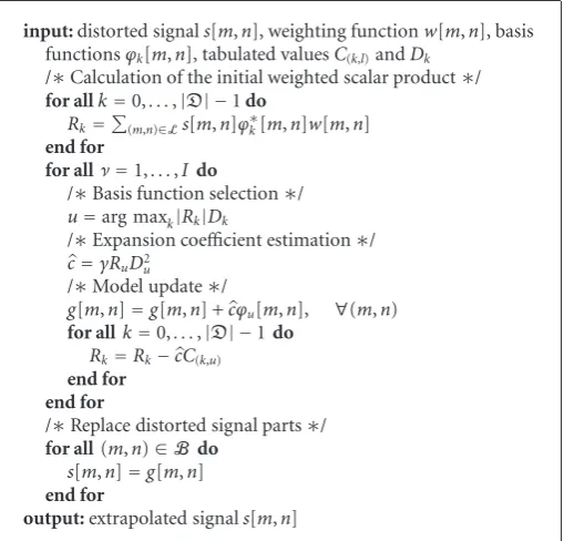
input:distorted signals[m,n], weighting functionw[m,n], basis functionsϕk[m,n], tabulated valuesC(k,l)andDk
/∗Calculation of the initial weighted scalar product∗/
for allk=0,. . .,| | −1do
Rk=(m,n)∈Ls[m,n]ϕ∗k[m,n]w[m,n]
end for
for allν=1,. . .,Ido
/∗Basis function selection∗/
u=arg maxk|Rk|Dk
/∗Expansion coefficient estimation∗/
c=γRuD2u
/∗Model update∗/
g[m,n]=g[m,n] +cϕu[m,n], ∀(m,n)
for allk=0,. . .,| | −1do
Rk=Rk−cC (k,u)
end for end for
/∗Replace distorted signal parts∗/
for all(m,n)∈B do
s[m,n]=g[m,n]
end for
output:extrapolated signals[m,n]
Algorithm3: Fast Selective Extrapolation for arbitrary basis functions.
5. Results for Arbitrary Basis Functions
In order to support the complexity evaluation from the previous section, the processing time for SE and FaSE is further examined. The first results presented are for arbitrary two-dimensional basis functions. In this case, only the original SE and the novel FaSE can be used, as transform domain algorithms like FSE cannot deal with arbitrary basis functions. For the runtime evaluation, the model generation has been implemented in C, compiled with gcc 4.3.2 and optimizations -O3, and the simulations have been carried out on an Intel Core2 Quad @ 2.83 GHz, equipped with 8 GB RAM. In order to reduce the influence from the operating system, multiple runs of the simulations have been conducted and the computation has been limited to the usage of only one single core.
For the simulations, a block of size 16 ×16 samples is extrapolated from its surrounding samples. Furthermore, different sizes of extrapolation areaLbetween 48×48 and 96×96 samples are regarded. Figure4 shows the extrap-olation time per block for different numbers of candidate basis functions and for 250 iterations performed for model generation. For this plot, the cardinality of the dictionary is selected to be of the same size as the extrapolation area. Thus,varies between|| = 2304 basis functions of size
48×48 and || = 9216 basis functions of size 96×96.
Comparing the two curves of SE and FaSE, one can easily recognize that FaSE is about 250 times faster than the original SE, independently of the problem size. This is due to the fact that for FaSE the computationally expensive weighted scalar products only have to be evaluated once, namely, prior to the first iteration. In the later iterations, the expensive steps can be avoided by making use of the tabulated values and
106 107 108 109 1010 1011 1012
Iterations
Oper
ations
SE FaSE
Table generation
0 500 1000 1500 2000 2500 3000 3500 4000
Figure3: Operations per block for model generation by SE and FaSE and operations necessary for generating tabulatedC(k,l) and Dk. For comparison, the operations for generating the tables are
drawn over the complete iterations range although they have to be calculated only once. Spatial sizesM = 64 andN = 64 and dictionary size| | =4096.
2000 3000 4000 5000 6000 7000 8000 9000 10−1
10−2
10−3 100 101
CPU-time/block
(s)
SE FaSE
Dictionary size|D| 102
Figure 4: Processing time over dictionary size for 2D model generation with arbitrary real-valued basis functions and 250 iterations. The size of the extrapolation area is chosen so thatMN= | |holds for every data point.
0 50 100 150 200 250
100 101
10−2
CPU-time/block
(s)
SE FaSE
Iterations 10−1
Figure5: Processing time over iterations for 2D model generation with arbitrary real-valued basis functions of size 64×64 and dictionary size| | =4096.
for an extrapolation scenario of size 64×64 samples. Taking into account the logarithmic axis, one can recognize that the processing time per block more or less linearly increases for SE, whereas for FaSE the processing time per block increases only very slowly. The results correspond well to the analytical complexity evaluation, and the speed gain of FaSE over SE is of the same magnitude as shown in the previous section. Apparently, Figure 3 cannot be directly translated into the processing time shown in Figure 5, since not all regarded operations consume the same processing time and since the analytical evaluation cannot account for optimizations introduced by the compiler.
Figure 6 shows the processing time for generating the tables for different dictionary sizes || and for different
Table2: Average results for extrapolation of 126 blocks of size 16×
16 samples in every image of the Kodak test image database.
Algorithm PSNR Processing time per block TV [17] 22.40 dB 0.54 sec SFG [18] 23.63 dB 15.29 sec SDI [19] 21.60 dB 0.0003 sec
FaSE 23.82 dB 0.38 sec
0.2 0.4 0.6 0.8 1 1.2 1.4 1.6 1.8 2 101
102 103
CPU-time
(s)
MN=48×48
MN=56×56
MN=80×80
MN=96×96
MN=64×64
Dictionary size|D| ·104
Figure6: Processing time for generating tables over dictionary size
| |for extrapolation areas of different sizesMN.
sizes of extrapolation areaL. Comparing these results with the ones shown in Figure 5 one can recognize that for an extrapolation area of size 64×64, a dictionary size of
|| =4096 and 250 iterations, the table generation only
takes as long as SE would roughly need for extrapolating 6 blocks. This corresponds well to the theoretical results presented in the analytical evaluation. The discrepancy follows from the fact that different operations consume unequal amounts of processing time while in the analytical evaluation only the absolute number of operations has been counted.
FaSE provides the highest extrapolation quality among the considered algorithms only with SFG coming close. But at the same time, it is the second fastest algorithm.
6. Modifications for Transform-Based
Basis Function Sets
As aforementioned, for FaSE the weighted scalar products only have to be evaluated prior to the first iteration. In the case that the regarded basis function set contains a subset of basis functions that emanate from a discrete transform as for example, functions of the DCT or the DFT, the explicit evaluation of the weighted scalar products can be simplified by replacing the summation over the product between the weighted signal and the basis function by the corresponding transform coefficient of the weighted signal which can be achieved through a fast transform. To give an example, the idea that the basis function set contains some basis functions which emanate from the DFT will be extended. In this case, a basis function is defined by
ϕk[m,n]=ej(2π/M)μkmej(2π/N)ηkn (21)
with vertical frequencyμkand horizontal frequencyηk. Then, the summation from (12) can be expressed by the DFT
(m,n)∈L
s[m,n]ϕ∗k[m,n]w[m,n]=DFT{s[m,n]w[m,n]}|μk,ηk
(22)
at frequency μk,ηk. Thus, the weighted scalar products for many basis functions can be efficiently evaluated simul-taneously by making use of fast transforms like the Fast Fourier Transform [20] or, respectively, a fast transform that is appropriate to the regarded basis functions. It has to be noted that the utilization of fast transforms is only reasonable if a large number of transform domain coefficients has to be calculated at the same time. The fast transforms only speed up the parallel calculation of many coefficients. The calculation of just a single coefficient would take as long as the explicit evaluation of the weighted scalar product. The above-described property could also be used for speeding up the table generation in (16). Regarding again the example of a subset of DFT basis functions, the product between a basis function and a conjugate complex second one is equal to a basis function where the horizontal and vertical frequency results from the difference of the original frequencies:
ϕ∗
k[m,n]ϕl[m,n]
=e−j(2π/M)μkme−j(2π/N)ηknej(2π/M)μlmej(2π/N)ηln
=ej(2π/M)(μl−μk)mej(2π/N)(ηl−ηk)n.
(23)
Hence, (16) can also be expressed by the corresponding coefficients from the DFT. For other transform-based basis function sets, similar properties exist.
In addition to the results for arbitrary basis functions shown in Section 5, the performance of FaSE and SE is compared to a transform domain algorithm. For this, FSE
**
* *
* * *
*
*
*
*
*
0 100 200 300 400 500
Iterations 10−4
10−3 10−2 10−1 100 101
CPU-time/block
(s)
SE FSE FaSE
Figure7: Processing time over iterations for 2D model generation with DFT basis functions,| | =4096.
is regarded that utilizes Fourier functions for extrapola-tion. Here the circumstance has to be considered, that, as described in [8], FSE does not generate a complex-valued model. FSE selects in every iteration step one basis function and its corresponding conjugate complex one, in such a way that the model is always real-valued. Hence, in most cases two basis functions are selected in an iteration, with the exception of the real-valued constant basis function and the function with the highest possible alternation. Thus, the number of iterations has to be doubled for SE and FaSE for a fair comparison as they select only one basis function per iteration. Figure7shows the processing time per block for the different approaches with|| = 4096 Fourier basis
functions of size 64×64. For these simulations, the initial scalar products for FaSE are expressed by the transform coefficients according to (22). Although FaSE needs twice the number of iterations as FSE for generating the model, it is still significantly faster than FSE and furthermore several magnitudes faster than the original spatial domain SE.
7. Conclusion
Within the scope of this contribution, we presented Fast Selective Extrapolation for image and video signal extrap-olation. For this, Selective Extrapolation, a powerful signal extrapolation algorithm has been reviewed and its most complex parts have been identified. The novel algorithm behaves mathematically identical to the original algorithm but is able to outspeed the original algorithm by several decades by effectively trading memory consumption versus processing time. Furthermore, the novel algorithm is able to outperform existent fast transform domain extrapolation algorithms which are even limited to certain basis function sets. With that, it opens the door for further research on car-rying out the extrapolation with different basis function sets. Up to now, the extrapolation only has been computationally manageable for special basis function sets that are based on discrete transforms. But by using Fast Selective Extrap-olation, the extrapolation can be carried out for arbitrary basis functions which may even be only numerically defined. This ability allows for further research on extrapolation with signal adapted basis functions, obtained through the Karhunen-Lo`eve Transform [21, 22], which has not been computationally feasible up to now.
Although the algorithm has been introduced only for two-dimensional data sets, it can be extended straightfor-wardly to three dimensions by making use of the ideas from [23] and four dimensions by using [24]. There, a three-dimensional or, respectively, a four-dimensional model is generated in the same way as described above for two dimensions.
References
[1] T. Stockhammer and M. M. Hannuksela, “H.264/AVC video for wireless transmission,” IEEE Wireless Communications, vol. 12, no. 4, pp. 6–13, 2005.
[2] I. Richardson,H.264 and MPEG-4 Video Compression, John Wiley & Sons, West Sussex, UK, 2003.
[3] B. A. Olshausen and D. J. Field, “Sparse coding with an overcomplete basis set: a strategy employed by V1?”Vision Research, vol. 37, no. 23, pp. 3311–3325, 1997.
[4] E. Cand`es, N. Braun, and M. Wakin, “Sparse signal and image recovery from compressive samples,” inProceedings of the 4th IEEE International Symposium on Biomedical Imaging (ISBI ’07), pp. 976–979, April 2007.
[5] J. A. Tropp, “Greed is good: algorithmic results for sparse approximation,” IEEE Transactions on Information Theory, vol. 50, no. 10, pp. 2231–2242, 2004.
[6] V. N. Temlyakov, “Weak greedy algorithms,” Advances in Computational Mathematics, vol. 12, no. 2-3, pp. 213–227, 2000.
[7] S. G. Mallat and Z. Zhang, “Matching pursuits with time-frequency dictionaries,”IEEE Transactions on Signal Process-ing, vol. 41, no. 12, pp. 3397–3415, 1993.
[8] A. Kaup, K. Meisinger, and T. Aach, “Frequency selective signal extrapolation with applications to error concealment in image communication,”International Journal of Electronics and Communications, vol. 59, no. 3, pp. 147–156, 2005.
[9] J. L. Herraiz, S. Espa˜na, E. Vicente et al., “Frequency selective signal extrapolation for compensation of missing sata in sino-grams,” inProceedings of the IEEE Nuclear Science Symposium Conference Record (NSS/MIC ’08), pp. 4299–4302, October 2008.
[10] M. Friebe and A. Kaup, “Fading techniques for error concealment in block-based video decoding systems,”IEEE Transactions on Broadcasting, vol. 53, no. 1, pp. 286–295, 2007. [11] J. Cooley, P. Lewis, and P. Welch, “The finite Fourier trans-form,”IEEE Transactions on Audio and Electroacoustics, vol. 17, no. 2, pp. 77–85, 1969.
[12] N. Ahmed, T. Natarajan, and K. R. Rao, “Discrete cosine transfom,”IEEE Transactions on Computers, vol. 23, pp. 90–93, 1974.
[13] J. L. Walsh, “A closed set of orthogonal functions,”American Journal of Mathematics, vol. 55, pp. 5–24, 1923.
[14] K. Meisinger and A. Kaup, “Minimizing a weighted error criterion for spatial error concealment of missing image data,” inProceedings of the International Conference on Image Processing (ICIP ’04), vol. 5, pp. 813–816, 2004.
[15] J. Seiler, K. Meisinger, and A. Kaup, “Orthogonality deficiency compensation for improved frequency selective image extrap-olation,” inProceedings of the Picture Coding Symposium (PCS ’07), Lisboa, Portugal, 2007.
[16] J. Seiler and A. Kaup, “Fast orthogonality deficiency compen-sation for improved frequency selective image extrapolation,” inProceedings of the IEEE International Conference on Acous-tics, Speech and Signal Processing (ICASSP ’08), pp. 781–784, 2008.
[17] J. Dahl, P. C. Hansen, S. H. Jensen, and T. L. Jensen, “Algo-rithms and software for total variation image reconstruction via first-order methods,”Numerical Algorithms, vol. 53, no. 1, pp. 67–92, 2010.
[18] X. Li, “Variational bayesian image processing on stochastic fac-tor graphs,” inProceedings of the IEEE International Conference on Image Processing (ICIP ’08), pp. 1748–1751, October 2008. [19] Z. Alkachouh and M. G. Bellanger, “Fast DCT-based spatial
domain interpolation of blocks in images,”IEEE Transactions on Image Processing, vol. 9, no. 4, pp. 729–732, 2000.
[20] J. Cooley and J. Tukey, “An algorithm for the machine calcula-tion of complex Fourier series,”Mathematics of Computation, vol. 19, no. 90, pp. 297–301, 1965.
[21] K. Karhunen, “ ¨Uber lineare Methoden in der Wahrschein-lichkeitsrechnung,”Annales Academiae Scientiarum Fennicae, vol. 37, pp. 3–79, 1947.
[22] M. Lo´eve, “Al´eatoires de second order,” inProcessus Stochas-tiques et Moevement Brownien, P. L´evy, Ed., Hermann, Paris, France, 1948.
[23] K. Meisinger and A. Kaup, “Spatiotemporal selective extrapo-lation for 3-D signals and its applications in video communi-cations,”IEEE Transactions on Image Processing, vol. 16, no. 9, pp. 2348–2360, 2007.
[24] U. Fecker, J. Seiler, and A. Kaup, “4-D frequency selective extrapolation for error concealment in multi-view video,” in