R E S E A R C H
Open Access
Modeling and optimization of the line-driver
power consumption in xDSL systems
Martin Wolkerstorfer
1*, Steffen Trautmann
2, Tomas Nordstr ¨om
1,3and Bakti D Putra
1Abstract
Optimization of the power spectrum alleviates the crosstalk noise in digital subscriber lines (DSL) and thereby reduces their power consumption at present. In order to truly assess the DSL system power consumption, this article presents realistic line driver (LD) power consumption models. These are applicable to any DSL system and extend previous models by parameterizing various circuit-level non-idealities. Based on the model of a class-AB LD we analyze the multi-user power spectrum optimization problem and propose novel algorithms for its global or approximate solution. The thereby obtained simulation results support our claim that this problem can be simplified with negligible performance loss by neglecting the LD model. This motivates the usage of established spectral optimization algorithms, which are shown to significantly reduce the LD power consumption compared to static spectrum management.
Keywords: Digital subscriber lines, Energy-efficient, Line driver, Optimization
Introduction
This article analyzes the modeling and optimization of the power consumption in multi-carrier digital sub-scriber line (DSL) transceivers. The line-driver (LD) power consumption accounts for the largest part in the DSL power budget and scales with the transmit power (TP) [1-3]. With few exceptions [2,4,5], previous study has therefore focussed on minimizing the transmit sum-power [3,6-8] through sum-power spectral optimization, also known as dynamic spectrum management (DSM) [9]. A key feature of this objective is its separability by subcarriers, which is a prerequisite for the Lagrange decomposition [10] of the DSM problem. This decom-position results in low-complexity and even distributed DSM implementations [11-13].
We hypothesize that although TP minimization does not assume knowledge of the underlying LD power con-sumption, it achieves energy-efficiency at a negligible per-formance loss compared to a TP optimization taking the LD explicitly into account. In order to support this claim and to realistically assess energy savings by DSM it is indispensable to have an accurate model of the LD power
*Correspondence: [email protected]
1FTW Telecommunications Research Center Vienna, Donau-City-Straße1, A-1220 Vienna, Austria
Full list of author information is available at the end of the article
consumption as a function of the TP. Hence, after provid-ing more background information in Section ‘Background information’, we begin in Section ‘Line driver models’ by deriving accurate such models, which are applicable for any DSL technology and different LD classes. While we deem a proof of our hypothesis intractable, we exemplar-ily provide analytical and numerical evidence supporting our hypothesis based on the proposed enhanced class-AB LD model in Sections ‘Optimization models and analysis’ and ‘Empirical optimization study’, respectively. For that purpose we propose two novel numerical approaches for LD power optimization which are based on successive geometric programming (GP) [14,15] and difference-of-convex-functions programming (DCP) [16], respectively. These techniques help us to motivate the selected scenario for simulation of a DSL network with realistic parameters under the two DSM heuristics in [2,3], cf. the introduc-tion in Secintroduc-tion ‘Empirical optimizaintroduc-tion study’ for a more concise overview of our contributions. The results are rounded off in Section ‘Average performance evaluation’ by simulations demonstrating the LD power saving poten-tial by energy-efficient multi-user DSM compared to static spectrum management and rate-maximizing DSM. Our conclusions are provided in Section ‘Conclusions’.
Background information Energy-efficiency in DSL
In the last ten years, the power consumption of informa-tion and communicainforma-tion technology (ICT) has become an issue on top of our agendas, reflecting our concern on global warming, CO2 emissions and energy sustainability. The telecommunication sector is responsible for 25% of the ICT’s energy consumption [17] and therefore energy efficiency has naturally become an issue for industry, stan-dardization, as well as governmental bodies. For example, the share of the fixed broadband access in the telco’s energy consumption for 2020 is estimated at around 14% [17]. A related initiative by the European commission aims at a power reduction of 50% in broadband equipment by 2015 [18].
The power consumption of a DSL transceiver can be divided according to its three major parts: the digital front-end(the modem’s digital signal processing); the ana-log front-end(responsible for the conversion between the analog and the digital domain, including filters); and the line driver(the power amplifier driving the line). Depend-ing on the used transmission profile (e.g., bandwidth) the LD power consumption can be somewhere between 30% and 60% of the modem’s total power consumption [1-3]. The main focus for energy saving in DSL therefore lies on the LD power consumption [1,4]. Approaches for reduc-ing the power consumption in DSL can be classified into three categories [19]: the optimization of hardware com-ponents; dynamic rate adaptation (e.g., by spectral opti-mization); and low-power modes. Our focus is on the first two approaches, as we a) model the power consumption of an energy-efficient LD type, and b) study energy-efficient DSM based on derived LD power consumption models, leading to lowered transmit rates. We refer to [20,21] for an introduction to LD design for DSL and to [1,22-25] for an overview of various energy saving techniques for DSL.
Line driver modeling
Current DSL systems rely on so called class-AB LDs as these provide a high degree of linearity over a large signal bandwidth. The main drawback of this type of amplifier however lies in its relatively low efficiency. Fur-thermore, the typical DSL signal exhibits a high crest factor (CF) with high peak values in comparison to its root-mean-square (rms) value. Even though those peak values occur with very low probability, the fixed supply voltage of a Class-AB LD must be sufficiently high to provide distortion-free amplification of the highest signal peaks. This implies that significant power savings could be obtained by modulating the supply voltage to follow the envelope of the amplified signal, as done in so-called class-H LDs. Class-G LDs [20] are class-AB LDs where the supply rail is switched, e.g., between a lower and a higher voltage levelVL andVH, respectively. The design
of a class-G LD can be differentiated by whether multi-ple supplies or internal charge pumps are used to provide the multiple supply voltages. In the former design the sec-ond supply voltage is typically not directly available on a DSL line card. An additional, costly DC-DC converter is required which must be included in the LD efficiency cal-culation. A class-H LD can be seen as a class-G LD with an infinite number of supply rails, consequently leading to a higher efficiency at the cost of a more complicated supply design. Altogether we consider the class-G design based on internal charge pumps as the most promising compromise between efficiency and complexity.
As motivated in Section ‘Introduction’, for the evalu-ation and optimizevalu-ation of the LD power consumption a realistic functional model is needed which maps the modem’s TP to its LD power consumption. An empirical model based on power measurements of a class-AB LD in ADSL2+ was presented in [2]. However, this model is not applicable to other DSL technologies or systems with different physical parameters. A circuit-level model for an LD of class-AB and G with two supplies has been pre-sented in [4], based on the models in [26]. However, these models do not precisely account for the non-idealities of the voltage supply chain [27] (e.g., transformer loss, impedance synthesize factor, etc.) and the power loss in the hybrid circuit. Therefore, in Section ‘Class-AB line-driver power model’, we derive an enhanced class-AB LD power consumption model based on [26] that can be applied to any DSL profile, and in Section ‘Class-G line-driver power model’, we propose a novel model for a class-G LD with charge pumps.
Line driver models
Class-AB line-driver power model
In this section, we enhance the functional class-AB LD model in [26] based on a circuit analysis, cf. Figure 1. The total power consumed by a class-AB LD is given as
PLD(AB)=Pu+Pdiss+PHybrid, (1)
wherePuis the output power measured at the LD output
of a line indexed byu ∈ U,Pdissis the total power
dissi-pated inside the LD, andPHybridis the power consumed
by the hybrid circuit. The level ofPHybridstrongly depends
on the hybrid implementation and topology and ranges from a few mW to several tens of mW. By the reformula-tion detailed in Appendix 1 the LD power consumpreformula-tion in (1) can be equivalently written as
PLD(AB)=Vs·
IQ+
2 π
Pu
Rline
+PHybrid, (2)
where Vs is the supply voltage of the LD, IQ is the
qui-escent current, andRline as defined in Appendix 1 is the transformed resistance of the line, cf. Figure 1. In the ideal case the supply voltageVs can be designed to cover the
output voltage swing CF·Vrms,idealdescribed by the
sig-nal crest factorCF and the ideal rms LD output voltage Vrms,ideal[26].
However, a more realistic representation of Vs should
include several impairments that will generally be present in real implementations and significantly influence the LD efficiency:
1) The achievable signal swing at the LD output is reduced from its theoretical maximum valueVsby a voltage dropVdrop. Its value is typically in the range between 2 and 4 V, and determined by the design and the underlying technology of the LD output stage. 2) The resistances of the copper coils and other
non-idealities cause an additional voltage drop over the transformer. This loss in effective signal power on the line is called transformer lossTLand can reach 0.2 to 0.5 dB for EP5 and EP7 transformers as used in xDSL central office (CO) applications. 3) Another voltage drop occurs in the termination
circuitry. Impedance synthesis is a commonly used concept in LD system integration [28] to reduce this
loss. More precisely, only a small part of the effective receive signal termination is provided by an external resistor, while the main part is actively generated by the LD itself. The impedance synthesis factorm- that is the ratio between the external resistor value and the over-all termination resistance - also determines the receive signal attenuation and cannot be made arbitrarily small. Therefore, a voltage drop by a factor
m/(m+1)must be included in the calculation of the required LD supply voltage. While for VDSL2 systems a reasonable choice ofmlies in the range from 3 to 6, for pure ADSL/ADSL2+ systems a more aggressive choice ofmin the range from 6 to 20 is possible.
Using Vrms,ideal =
Pu·Rline these additional factors
can be accommodated in the form
Vs=CF·
ˆ
Pu·Rline·TL·
m+1
m +VDrop, (3)
where Pˆu is the maximum transmitted power. Figure 2
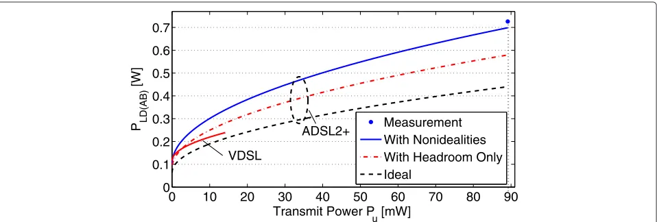
depicts an exemplary measurement of a real ADSL2+ LD’s power consumption, as well as the class-AB LD power consumption modelain (2), using (a) the mentioned ideal relationVs = CF·Vrms,ideal, (b) the relationVs = CF·
Vrms,ideal+Vdropwith headroomVdropas used in [4], and
(c) the relation derived in (3). From this plot it is visible that there is a considerable amount of LD power con-sumption that has not been taken into account by previous models.
Based on the wide deployment of class-AB LDs and the simple functional shape of our model we will focus on this LD type when analyzing the effect of the LD on energy-efficient DSM in Sections ‘Optimization models and analysis’, ‘Empirical optimization study’, and ‘Average performance evaluation’. Another energy-saving approach mentioned in Section ‘Energy-efficiency in DSL’ is the
0 10 20 30 40 50 60 70 80 90
0 0.1 0.2 0.3 0.4 0.5 0.6 0.7
Transmit Power P
u [mW]
P LD(AB)
[W]
Measurement With Nonidealities With Headroom Only Ideal
VDSL
ADSL2+
deployment of more energy-efficient LDs, as analyzed in the following section.
Class-G line-driver power model
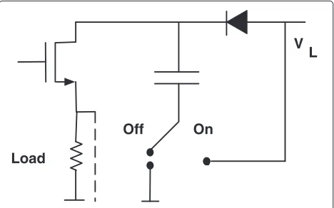
Based on our discussion in Section ‘Line driver modeling’, we study in this section class-G LDs with a set of inter-nal charge pumps. We refer to Appendix 2 for a model of an LD with two supply voltages that includes the non-idealities discussed in Section ‘Class-AB line-driver power model’ into the model in [4,26]. The basic principle of a charge pump is exemplified in Figure 3. A pair of such charge pumps is used to generate the high class-G sup-ply voltageVH from a single LD supply voltage which at
the same time serves as the low class-G supply voltage VL. Under ideal conditions, a maximum voltage ratio of
VH/VL = 3 can be achieved. However, taking
techno-logical limitations and various internal voltage drops into account, assuming a ratio ofVH/VL ≈ 2 is more
realis-tic. The total power consumption of a class-G LD with internal charge pumps is defined as
PLD(G-CP)=PLow,CP+PHigh,CP+PQ,CP+PHybrid, (4)
wherePLow,CPis the LD power consumption value of an
equivalent class-AB LD running continuously at the low voltage supply, andPHigh,CPrefers to the additional power
consumption when the LD is switching to the high volt-age supply.PQ,CPis the quiescent power dissipation. The
voltage levelVHis thought of as the summation ofVLand
VH −VL, with the latter being generated by the charge
pumps when needed. The consumed LD power at the low voltageVLis in analogy to (2) defined as
PLow,CP=VL·
2 π
Pu
Rline. (5)
Extending the ideal rms voltageVrms,ideal=
Pu·Rline
with the non-idealities of Section ‘Class-AB line-driver
V L
Off On
Load
Figure 3Class-G LD: Basic principle behind an internal charge pump.
power model’ we obtain the rms LD output voltage (that is, before impedance synthesis and transformer) as
Vrms=
PuRline·TL·
m+1
m . (6)
In analogy to the ideal class-G case [26] the mean average deviation (MAD) of the LD output voltage for the cases when the Gaussian distributed output signal is below and above the thresholdVth=(VL−Vdrop)is given
as
VMAD,Low =
2 πVrms
⎛ ⎝1−e−
V2
th 2Vrms2
⎞
⎠, (7)
and
VMAD,High =
2 πVrmse
− Vth2
2Vrms2 , (8)
respectively. Note that the fraction of timeμcp(Pu)∈[ 0, 1]
the charge pump is used is higher than the time the out-put signal exceeds the thresholdVth, the reason being the
additional ramp-up / ramp-down phases between the low and the high supply. Therefore the output signal’s MAD during charge pump usage is a combination of that when the signal is below and aboveVth, respectively, weighted
by the corresponding probabilities. The output signal’s MAD under the assumption of operating below and above the threshold is given by VMAD,Low/(1−2Q(VVrmsth))and
VMAD,High/(2Q(VrmsVth), respectively. Correspondingly we
define the dynamic powerPHigh,CPas
PHigh,CP= (9)
VH−VL
RlineTLmm+1
μA·VMAD,Low+μB·VMAD,High
·ρ,
where
μA= μcp(Pu)−2Q( Vth Vrms)
1−2Q(VrmsVth ) , (10)
μB=1,Q(·)is the Q-function,ρis the recharge loss, and
the termRlineTLmm+1represents the total resistance at the LD output. Comparing the total dynamic power (the sum of (5) and (9)) to that under a class-G design with two sup-plies (the sum of (30a) and (31) in Appendix 2) we find that the latter one is obtained by settingμA = 0 andρ = 1. We emphasize thatμcp(Pu)depends not only on the
out-put power, but, for example, also on the transformer ratio, the DSL profile, or the way in which the charge pump is loaded. The quiescent power consists, differently to that in class-AB LDs, of three main components, given as
The termPQ,Low=VL·IQis the quiescent power
dissi-pation of an equivalent class-AB LD continuously working atVL. The additional quiescent power dissipation of the
LD when working at the high voltage supply is defined as
PQ,High=(VH−VL)·IQ·μcp(Pu)·ρ. (12)
The third term in (11) splits into
PQ,classG= (13)
VL+(VH−VL)·μcp(Pu)·ρ
·IQ,classG+LclassG,
whereIQ,classGis the additional quiescent current in
class-G mode andLclassG[W] refers to further fixed losses in the
class-G circuitry.
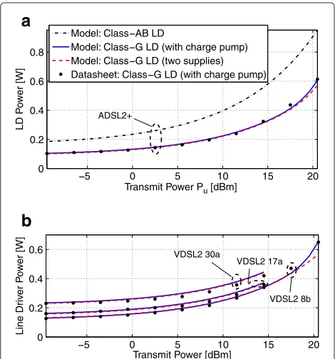
In Figure 4, we compare the power consumption data provided for a real class-G LD with charge pumps in [29] to the three discussed LD models: our model of a class-G LD with charge pumps in this section, the model of a class-G LD with two power supplies in Appendix 2, and the model of a class-AB LD modeled by Equations (2) and (3), respectivelyb. In Figure 4a we see that under an ADSL2+ profile the power consumption predicted by our model of a class-G LD with charge pumps lies between that
calcu-5 0 5 10 15 20 0
0.2 0.4 0.6 0.8
Transmit Power Pu [dBm]
LD P
o
w
er [W]
Model: Class AB LD
Model: Class G LD (with charge pump) Model: Class G LD (two supplies) Datasheet: Class G LD (with charge pump)
ADSL2+
a
5 0 5 10 15 20 0
0.2 0.4 0.6
Transmit Power [dBm]
Line Dr
iv
er P
o
w
er [W] VDSL2 30a
VDSL2 8b VDSL2 17a
b
Figure 4Comparison of class-G LD power models to a real class-G LD with charge pumps.Our model of a class-G LD with charge pumps shows a higher (lower) power consumption compared to an ideal class-G (class-AB) design. It accounts for additional power losses at high transmit powers that are also observable in a real class-G implementation. However, all three LD power models show a similar shape as a function of transmit powerPubelow 14.5dBm.
lated by the models of a class-AB LD and a class-G LD with two supplies. Figure 4b shows that the class-G LD models lead to similar power estimates for transmit pow-ers below 14.5dBm. This is explicable by the fact that a low transmit power leads to low probabilitiesμcp(Pu)and μ2S(Pu)of using the high supply in the class-G LD with
charge pumps and with two supplies (see Appendix 2), respectively. Correspondingly we can approximate the power consumption of a class-G LD for low transmit power values by that of a class-AB LD in (5) that operates at the low supply voltage. However, near the maximum output power the novel class-G LD model with charge pumps significantly deviates from the class-G LD model with two supplies, similarly as the consumption of the real LD described in [29]. For example, at the maximum trans-mit power of 20.5dBm the two-supply class-G LD model underestimates the power consumption of the LD in [29] by as much as 44mW for ADSL2+ or 83mW for VDSL2 8b. Regarding for instance the curves for VDSL2 30a we find that the real consumption values are partially below the class-G LD models for higher transmit powers. This can be explained by the deviation of the quiescent current into the load [28] which is circuit and transmit power depen-dent. Differently, all the presented LD models (as well as those in [4,26]) assume a constant quiescent current IQ
that is independent of the transmit power.
In summary, the class-G design with charge pumps yields substantial energy savings compared to a class-AB LD while sparing us the DC-DC conversion needed for class-G LDs with two supplies. Furthermore, the pre-sented LD power models have a qualitatively similar func-tional shape for transmit power values below 14.5dBm as they are all based on the elementary class-AB power relation in (2). In the following sections, we focus on the class-AB LD and analyze our hypothesis of Section ‘Introduction’ on the difference between LD power and TP optimization.
Optimization models and analysis
In this section, we want to formally develop some insight into whena difference between LD power and TP opti-mization in terms of the achieved class-AB LD power might occur, how large it is, and whether this difference truly occurs under realistic network conditions.
DSL system model and notation
of all users jointly. The achievable rate per DMT-symbol ruc(pc) for useru ∈ U = {1,. . .,U}on subcarrier c ∈
C = {1,. . .,C} as a function of the signal to interfer-ence and noise ratio (SINR) is modeled by the common gap-approximation [30]
rcu(pc)=log2 ⎛ ⎜ ⎜ ⎜ ⎜ ⎝1+
Hcuupuc
i∈U\u
Hui c pic+Ncu
⎞ ⎟ ⎟ ⎟ ⎟
⎠, (14)
where pc =[p1c,. . .,pUc]T, puc is the power assigned to
subcarrier c of user u, and the terms Hcuu and Hcui are the direct channel transfer coefficient of user uand the cross-channel transfer coefficient from user i to user u on subcarrier c, respectively. DSM implementations in standard-compliant DSL systems, including crosstalk esti-mation functionality, have been reported in [31,32]. The term indicates the SNR-gap to capacity depending on the modulation scheme, the targeted bit-error rate, the coding gain, and the noise margins, whileNu
c represents
the total received background noise power on subcarrier cof useru, including white thermal noise, alien-crosstalk, and radio-frequency interference.
Based on Section ‘Line driver models’, the LD power consumption of a class-AB LD as a function of the total TPPu=c∈Cpuc of useruis given in the form
fuLD(Pu)= ˆwu
Pu+ ˘wu, (15)
where the parameterswˆu∈R+andw˘u ∈R+are depen-dent on the hardware and system modelc. In the following optimization study, we will use two key features of this function: a) it is monotonously increasing, and b) concave inPu(orpuc,c∈C, respectively).
Optimization problems
Similarly as in previous DSL studies [11,33] we mathemat-ically formulate the problem of minimizing the transmit sum-power in DSL in the form
JTP=minimize
puc,u∈U,c∈C
u∈U
c∈C
puc (16a)
subject to
c∈C
ruc(pc) Ru, ∀u∈U, (16b)
c∈C
puc ˆPu, ∀u∈U, (16c)
0≤puc ≤ ˆpuc, ∀c∈C,∀u∈U, (16d)
rcu(pc)≤ ˆB, ∀c∈C,∀u∈U, (16e)
where pˆcu,c ∈ C,u ∈ U, denotes the PSD mask, Bˆ the maximum number of bits that can be allocated to a single subcarrier, and Ru and Pˆu the target-rate per
DMT-symbol and the maximum sum-power of user u, respectively. In practice numerous other objectives may be targeted besides energy consumption, including for exam-ple sum-rate [33], fairness [34], service coverage [35], the energy-per-bit [8], or weighted combinations thereof [6]. However, our choice of focusing on energy-minimization subject to rate-constraints will allow us to study various defined rate combinations. Similarly to (16), based on the model in (15) the problem of minimizing the total LD power consumption in DSL can be stated as
JLD=minimize
pu c,u∈U,c∈C
u∈U
c∈C
pu
c (17a)
subject to Constraints (16b)–(16e), (17b)
where for simplicity of exposition we assume identical LD models for all users. This allows us to omit the added con-stantw˘uand the factorwˆu,u ∈ U, as they have no
influ-ence on the optimal solution. Note that the latter factors can easily be reintroduced under the numerical optimiza-tion approaches in Secoptimiza-tion ‘Empirical optimizaoptimiza-tion study ’. For instance, heterogeneous LD models are considered for the simulations in Section ‘An experiment in real-sized DSM problems using heuristics’. For brevity we will denote the optimal per-user sum-power values for the problems in (16) and (17) byPTP∈RU+andPLD∈RU+, respectively.
Analysis of the optimization problems in (16) and (17) Before turning to the numerical optimization of the
prob-lems in (16) and (17) we analyze their solutions and the difference between their solutions in terms of LD power independently of their exact solution value. To begin with we define the set of possible solutions (the “power-region”).
Definition 1(Power-region).The power-region associ-ated with the problems in (16) and (17) is defined as the set
P = {P∈RU| ∃puc,c∈C,u∈U,feasible for constraints (16b)–(16e),Pu=
c∈C
puc}. (18)
Proposition 1. The sum-power vectors PTP and PLD
the power-regionP as defined in (18), i.e.,P ∈ P,P = PTP,PPTPandP∈P,P=PLD,PPLD.
Proof.The proof simply follows from the monotonicity of the objectives in (16a) and (17a), respectively.
Proposition 1 also suggests a practical heuristic approach for LD power optimization, namely through a sequence of weighted sum-power minimizations with weights based on the projected gradients of the objective functionsfuLD(Pu), cf. [36] where a similar idea was applied
for a rate-utility maximization problem. However, while in [36] a non-concave maximization was performed over the rate-region, here we face a concaveminimizationproblem over the power-region.
The following proposition identifies the smallest lem instances where a difference between the two prob-lems in terms of LD power may occur, and which we will further study in Section ‘Empirical optimization study’.
Proposition 2.Differences between the optimal solu-tions of the problems in (16) and (17) in terms of LD power can only occur for U≥2and C≥2.
See Appendix 3 for a proof.
Next, we define the relative gain by LD power opti-mization in (17) compared to TP miniopti-mization in (16) as
ξ = ˆ
wu∈UPTP
u −
PLD u
ˆ
wu∈UPTP
u +U· ˘w
, (19)
where in the nominator we have the difference in LD power between the two optimization approaches we are interested in, and in the denominator the LD power under the TP minimization. In other words, the relative gain in (19) tells us how much more energy-efficient LD power optimization is compared to classical TP minimization. In the following we derive a bound onξ for any number of usersUand subcarriersCwith powerspucsumming to the total powerPu=c∈Cpuc. More precisely, we have
u∈U
PTP
u ≤JLD≤
u∈U
PTP
u , (20)
where the first inequality holds due to the monotonicity and concavity of the model in (15), and the optimality of
u∈UPuTP in (16), and the second inequality holds due
to feasibility of a solution to the problem in (16) for the problem in (17). Using (20) in (19) we obtain the bound
ξ ≤ ˆ
wu∈UPTP
u −
u∈UPTPu
ˆ
wu∈UPTP
u +U· ˘w
, (21)
which is only dependent on the solution of the problem in (16) and illustrated in Figure 5. Expanding our intu-ition from Proposintu-ition 2, we see that this simple bound does not allow for any LD power reduction by direct LD power optimization in (17) compared to TP minimization in (16) when all but one user transmit with very low power (e.g., below -20 dBm). Note however that Figure 5 does not allow us to make any conclusions on possible differ-ences when all lines operate in a high-power regime. For example, if the solution to the TP minimization problem in (16) demands all users to use maximum sum-power, by sum-power optimality in (16) the same must hold in the LD power minimization problem in (17) and so the differ-ence between the two must actually vanish, differently to what the bound in (21) indicates. Using Jensen’s inequal-ity we can even bound (21) independently of the solution
PTP, giving
ξ ≤
1−√1 U
⎛
⎜
⎝1+ w˘ √
U
ˆ
wu∈UPˆu ⎞ ⎟ ⎠
−1
. (22)
The gain ξ forU = 2 users is for instance bounded by 1−1/√U (≈ 30%). The bounds in (21) and (22) are identical whenPTPu = ˆPu=P,∀u∈U.
In this section, we have located the solutions of our two optimization problems on the boundary of a power-region and identified potentially insightful problem instances. In the following section, we will use this information to study the real gainξby directly optimizing the LD power model through numerical methods.
Empirical optimization study
We will use three approaches to obtain insights into the differences between TP and LD power minimiza-tion in terms of the LD power consumpminimiza-tion founded on the functional model in (15): The first one is based on an efficient but possibly suboptimal successive geometric
programming (GP) approximation used in order to iden-tify problem parameters under which differences between the optimal solutions of the two optimization problems occur. While it is known [15] that the TP optimization problem can be approached by GP, our contribution is to recognize this fact for the LD power optimization prob-lem. The second approach is based on the globally optimal solution of both problems in (16) and (17). Global opti-mality is a necessary property to study the power-region in Definition 1 and the location of the solutions to the problems in (16) and (17) in this region. Furthermore, it allows us to provide an exemplary scenario where prov-ably a difference between the solutions of the two opti-mization problems occurs. For solving these non-convex and rate-constrained LD power and TP optimization problems we found it necessary to develop a problem-specific algorithm. It deviates in various aspects from the approaches proposed for related rate-maximization problems in [37,38], e.g., it allows for an optimization over all subcarriers including a non-convex constraint set, and uses improved branching and bounding tech-niques. The third approach is by the heuristic succes-sive convex approximation algorithms proposed in [2,11], respectively. These two algorithms allow to study problem instances of realistic size and channel parameters.
DSM based on successive SINR-approximation and geometric programming
Geometric programs (GP) are a class of problems which is not convex but can easily be converted into a con-vex form by logarithmic transformations [14]. This opti-mization model was applied to power control in [15,39], where also successive GP approximations were proposed for non-convex problems based on monomial [14] or SINR approximations [11]. For a short introduction to GP and the corresponding problem transformation of the LD power optimization problem in (17) we refer to Appendix 4.
As mentioned above our motivation for applying suc-cessive GP is to solve numerous small problem instances (U = C = 2) in order to identify problem param-eters which lead to a substantial gain ξ by LD power optimization compared to TP optimization. We gener-ated numerous problem instances of (16) and (17) by setting Hc21 and Hc12 to all combinations out of the set {−90,−67.5,−45,−22.5, 0}dB, and for each of these com-binations forming all target-rate comcom-binations sampling the users’ possible rates at 20 equi-distant rate-levels from 0 to the maximum achievable rate (i.e., 400 rate-combinations)d. After running successive GP for the
prob-lems in (16) and (17) we re-initialize the algorithm with the obtained result for the respective other problem and keep the best solution found for each probleme. Also, we multiply the per-user sum-powers by a factor of 500
before applying the LD power model in order to obtain a more realistic estimate of the LD power savingsf. The
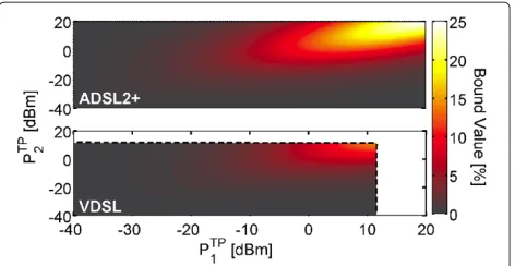
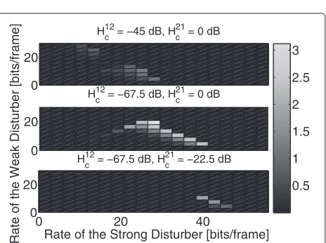
result of this experiment can be summarized as follows: Significant values ofξ occurred under unsymmetric set-tings of target-rates and crosstalk coefficients, especially so when the stronger disturber is the one having the larger target-rate, cf. Figure 6. Intuitively this kind of setup results in one user operating with low sum-power (where the derivative of the LD power model in (15) is high) while the user with the larger target-rate operates with higher sum-power (corresponding to a lower derivative of the LD power model in (15)). From a sum-power perspective it may make sense to allow the strong disturber to inter-fere with the weak disturber due to his higher target-rates. However, from an LD power perspective the user with the low target-rates is worth protecting more due to the larger derivative of the LD power model at low sum-power values, cf. the LD power model in Figure 2.
In the following section, we select a specific scenario based on these insights for further investigation.
Global solutions of non-convex LD power optimization problems using difference-of-convex-functions programming (DCP)
Difference-of-convex-functions programming (DCP) [40] is a widely applicable approach in global optimization where non-convex objective and constraint functions are reformulated as the difference of convex functions, cf. [37,38] for recent applications in power control. Simi-larly to the reformulation shown in [37,38] for a rate-maximization problem, the rate-constraints in (16b) can be equivalently written as
−
c∈C
rucpc+Ru=gu(p)−hu(p)≤0,u∈U, (23)
0 20
Rate of the Weak Disturber [bits/frame]
0 20
0 20 40
0 20
Rate of the Strong Disturber [bits/frame] 0.5 1 1.5 2 2.5 3
H12
c = −45 dB, H 21 c = 0 dB
H12c = −67.5 dB, H21c = −22.5 dB H12
c = −67.5 dB, H 21 c = 0 dB
where
gu(p)= −
c∈C
log
⎛
⎝Huuc pcu+
j∈U\{u}
Hujcpcj+Nuc
⎞ ⎠+Ru,
(24)
hu(p)= −
c∈C
log
⎛
⎝
j∈U\{u}
Hujcpcj+Nuc
⎞
⎠, u∈U,
(25)
are convex functions. Writing the objective in (17a) formally as 0 − h0(p) with convex function h0(p) =
−u∈U
c∈Cpuc we can write the problem in (17) as
the following DCP problem [40],
minimize
puc,u∈U,c∈C
−h0(p) (26a)
subject to gu(p)−hu(p)≤0, u∈U (26b)
Constraints (16c)–(16e). (26c)
While in previous applications of DCP in the area of power control [37,38] the problem was in fact solved as a concave minimization problem over a convex straint set, we have additionally complicating DCP con-straints in (26b). Correspondingly we developed a more general solution approach, namely a box-based branch-and-reduce algorithm initialized by a successive GP [15] solution, cf. Appendix 5 for details. Note that this DCP algorithm can similarly be applied to (optimally) solve the TP problem in (16).
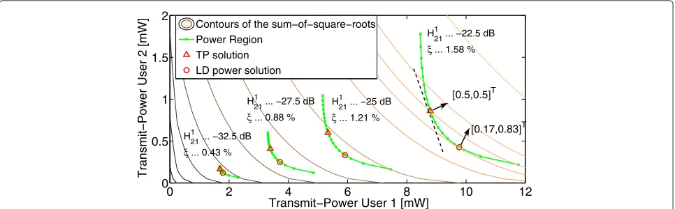
We use the developed global optimal algorithm to inves-tigate the power-region as given in Definition 1. For reasons of tractability we restrict ourselves to a specific scenario (U = C = 2) identified using the heuristic in Section ‘DSM based on successive SINR-approximation
and geometric programming’g. In Figure 7, we show the power-regions and the solutions of the problems in (16) and (17) for varying crosstalk parameter H21
c .
First, we see that both solutionsPTPandPLDlie on the power-region, as predicted by Proposition 1. However, the solutions lie on different contour lines of the function
u∈U√Pu, meaning that they provably differ in terms of
LD power consumption. While the TP solution minimizes [ 0.5, 0.5]·P over the power-region, the LD power opti-mal solution minimizes [ 0.17, 0.83]·P. In other words, the LD power optimum is attainable by a weighted sum-power optimization with specific weights. Searching for these weights is in fact the idea behind the projected gradient heuristic indicated in Section ‘Analysis of the optimization problems in (16) and (17)’. With a decreas-ing parameterH121 the needed sum-powers for constant target-rates decrease, leading to a decrease of the achiev-able gain ξ by LD power optimization compared to TP minimization, cf. Figure 7.
An experiment in real-sized DSM problems using heuristics In this section, we compare solutions obtained by two DSM heuristics and static spectrum management (SSM) in terms of their LD power: (a) the successive convex approximation algorithm [3] for the problem in (16) which is based on the convex approximationr˜uc(pc)of the
rate-functionrcu(pc)as given in Appendix 4 and introduced in
[11] for a rate-maximization problem in DSL; (b) the suc-cessive LP approximation algorithm in [2] for the problem in (17) which mainly differs from the above approxima-tion heuristic in that the approximaapproxima-tion is linear and the approximated problems are not solved iteratively but jointly for all users, and (c) single-user water-filling con-sidering a static background noise including the highest possible crosstalk noise based on the other systems trans-mitting at PSD mask. A novelty we introduce for the comparison of suboptimal DSM algorithms is that after
0 2 4 6 8 10 12
0 0.5 1 1.5 2
Transmit−Power User 1 [mW]
Transmit−Power User 2 [mW]
Contours of the sum−of−square−roots Power Region
TP solution LD power solution
H
21
1 ... −22.5 dB ξ ... 1.58 %
[0.5,0.5]T
[0.17,0.83]T
H
21 1
... −25 dB
ξ ... 1.21 % H1
21 ... −27.5 dB ξ ... 0.88 % H1
21 ... −32.5 dB ξ ... 0.43 %
obtaining the result of a DSM scheme we initialize the respective other DSM algorithm with this result and keep the best solutions in terms of LD power and TP objec-tive, respectively. The purpose of this strategy is to avoid the dependency of the comparison on the initialization which might have been chosen in favor of one of the algorithmsh. The difference to the initialization approach in Section ‘DSM based on successive SINR-approximation and geometric programming’ is that we cross-initialize two heuristics, while in Section ‘DSM based on successive SINR-approximation and geometric programming’ we applied a single heuristic to two different problems.
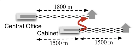
Based on the insights of the two previous sections we design a network scenario with realistic parameters where we would expect a difference in LD power between the two considered optimization approaches. This is with respect to the selected channel model (a 99% worst-case model [30]), the network topology (a near-far scenario with one CO deployed line and 7 cabinet deployed dis-turbers), the bandplan (showing strong crosstalk with the CO deployed line, see below), the target-rates (low rates for the CO deployed victim line and high rates for the cab-inet lines), and the selected DSL systems (the LD power model for the VDSL cabinet lines has a lower slope than that for the ADSL2+ CO line, cf. Figure 2). More precisely, we consider the near-far downstream scenario shown in Figure 8 with 8 lines deployed in the same cable bundle, where 7 VDSL lines are deployed from a cabinet and one ADSL2+ line is deployed from the CO. We set the param-eters of the ADSL2+ line in accordance with the standard in [41] (using the non-overlapping bandplan with ISDN in Annex A) and of the VDSL lines according to [42] with a total SNR gap of = 12.3 dB in both systemsi. The
assigned target-rates are 1, 2, or 3 Mbps and 10, 13, 16, or 19 Mbps for the CO and cabinet deployed lines, respec-tively, and we investigate all 12 combinations of these target-ratesj.
We observed that due to the heuristic nature of both algorithms the LD power optimization did not always give a better total LD power than the TP optimization (corre-sponding to a negative gainξ in (19)). In summary, the gain ξ in (19) was in the studied 12 scenarios between −0.01% and+0.01%. DSM gives a more substantial LD
Central Office Cabinet
1500 m 1800 m
1500 m
Figure 8Constructed network example with 7 cabinet-deployed lines disturbing a single CO-deployed line.
power reduction compared to SSM between 20% and 40%. While this result is no definite answer to whether or not LD power optimization makes a difference compared to TP optimization, it is another indication that in practice the difference may be assumed negligible, which motivates the simplification of the optimization in this direction. However, multi-user DSM bares a substantial potential for energy-reduction compared to SSM, as we shall study further in a larger set of scenarios in the following section.
Average performance evaluation
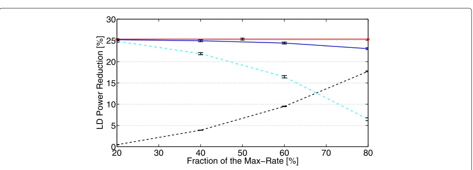
Differently to the previous section we will next study the possible LD power reduction by TP optimization (DSM) compared to SSM in 300randomlygenerated net-work topologies with simulation parameters as specified in Section ‘An experiment in real-sized DSM problems using heuristics’. More precisely, we study two deploy-ment scenarios, where the first one consists of 15 ADSL2+ lines with loop-lengths uniformly sampled between 800 m and 1600 m. The second type of scenarios consists of 15 VDSL cabinet-deployed lines with loop-lengths between 300 and 800 mk. We compare the TP optimization algo-rithm in [3] and the SSM algoalgo-rithm as described in the previous section. Target-rates are set by multiplying the (scenario dependent) maximum achievable per-user rates as achieved by the heuristic in [2] by factors of {0.2, 0.4, 0.6, 0, 8}. Differently to above, the crosstalk chan-nel model is based on measurements in [43], where we perform a random cable selection for each network sam-ple. Summarizing, the simulation setup does not exag-gerate the inter-user crosstalk (e.g., by near-far scenarios or worst-case crosstalk couplings) and therefore provides a realistic evaluation of the energy savings by multi-user DSM compared to SSM.
Next, we present the average LD power consumption results together with 99% confidence intervals according to a student t-test. The average LD power consumption in the ADSL2+ scenarios obtained by the sum-rate maximiz-ing DSM algorithm in [2] leads already to an LD power reduction compared to (spectral mask and sum-power constrained) full-power transmission of 38.70% (±0.97%), which has to be compared to the maximum possible sav-ings by TP reduction (which is obtained by reducing the TP to zero) of 85.69%. Hence, even rate-maximizing DSM can be regarded as an energy saving technology, as already argued in [44]. In the VDSL scenarios the sum-rate max-imization leads to an LD power reduction compared to full-power transmission of 9.10% (±0.46%). The maxi-mum possible savings are now only 32.14%, due to the lower sum-power constraint as enforced by the spectral mask, cf. the LD model for VDSL in Figure 2.
20 30 40 50 60 70 80 0
20 40 60 80
Fraction of the Max−Rate [%]
LD Power Reduction [%]
Zero TP vs. Max−Rate DSM EE−DSM vs. Max−Rate DSM EE−SSM vs. Max−Rate DSM EE−DSM vs. EE−SSM
Figure 9LD power savings achieved by various TP optimization strategies in ADSL2+.
scenarios multi-user DSM gives (on average) more than 70% LD power reduction at 80% of the maximum rates compared to sum-rate maximizing DSM, whereas SSM only results in less than 11% LD power reduction. Hence, DSM gives substantial improvements compared to SSM, most noticeable at higher rates. In the VDSL scenarios the conclusions are qualitatively similar. However, as shown in Figure 10, the LD power reduction at 80% of the max-imum rates is now only 23%, whereas SSM results in less than 7% LD power reduction.
Conclusions
We derive novel realistic models of the line-driver (LD) power consumption in class-AB and G LDs as a func-tion of the transmit power (TP) in digital subscriber lines (DSL). These models include non-idealities of the power supply and therefore result in more accurate, higher figures of LD power consumption. Based on the functional shape of the class-AB LD model we exemplarily study its optimization by dynamic spectrum management (DSM).
Multi-user DSM was seen to give substantial energy sav-ings compared to static spectrum management in a large set of DSL scenarios. Furthermore, through an empirical simulation study we were able to identify small DSM prob-lem instances where the TP and the LD power optima provably differ in terms of LD power consumption. How-ever, we were not able to reproduce this difference in sim-ulations for systems of practical size, which suggests that the multi-user DSM problem can be simplified by opti-mizing TP instead of LD power at negligible performance loss.
Appendix 1
Derivation of the class-AB LD model
In this appendix, we detail the derivation of (2) based on (1), adapted from [26]. The output power in (1) is defined as
Pu=
Vrms,ideal2
Rline , (27)
20 30 40 50 60 70 80
0 5 10 15 20 25 30
Fraction of the Max−Rate [%]
LD Power Reduction [%]
whereVrms,ideal=
E{|VO|2},VO∼N(0,Vrms,ideal2 )is the
normal distributed output voltage (cf. Figure 1), Rline = Rline/n2is the transformed resistance of the line, andnis
the transformer ratio. The average dissipated powerPdiss
can be decomposed into the quiescent powerPQand the
dissipated power associated with the voltage drop in the class-AB design [46], according to
Pdiss+Pu=PQ+E
(Vs− |VO|)|
VO|
Rline
+Pu (28a)
=PQ+
Vs
RlineE{|VO|} (28b)
=Vs·IQ+
Vs
Rline
2
πVrms,ideal, (28c)
whereVsis the supply voltage and in (28a) we use (27), cf.
[26] for details. Equation (2) derives by (1) and using (27) in (28c).
Appendix 2
Model of a class G LD with two supplies
The power consumption of a class-G LD with two supply voltages is given as
PLD(G−2S)=PLow,2S+PHigh,2S+PQ,2S+PHybrid, (29)
wherePLow,2SandPHigh,2Sare the consumed powers when
the supply voltage is VL and VH, respectively, PQ,2S = (VL(1−μ2S(Pu))+VHμ2S(Pu))·IQis the quiescent power,
andμ2S(Pu)∈[ 0, 1] is the fraction of time the high supply
voltage is active. Assuming a thresholdVth=(VL−Vdrop)
for switching between the two supplies, where Vdrop is
the voltage drop in the class-AB design, and that the LD’s output voltageVOis Gaussian distributed [26] with zero
mean and varianceV2
rms, we haveμ2S(Pu) = 2Q(VVrmsth),
Q(·) denoting the Q-function. Furthermore, PLow,2S is
computable as (see [26] for a similar derivation)
PLow,2S=
2VL
RlineTLmm+1
Vth
0
x √
2πVrms
e− x2
2Vrms2 dx
(30a)
=VL·
2 π
Pu
Rline ·
⎛ ⎝1−e
−(VL−Vdrop)2
2PuRline(TL mm+1)2 ⎞
⎠, (30b)
where the termRlineTLmm+1in (30a) accounts for the total LD output resistance, and in (30b) we use the definition ofVrmsin (6). Similarly, the power consumption when the
supply with the higher voltage levelVHis active is derived
as
PHigh,2S=VH·
2 π
Pu
Rline ·e
−(VL−Vdrop)2
2PuRline(TL mm+1)2
. (31)
These formulas are equivalent to those shown in [4,26], with the exception of the quiescent power calculation and the consideration of the resistance Rline at the primary transformer side, the voltage dropVdrop, the transformer
loss TL, and the synthesis factormin the computation of the voltage-level probabilities. Not included in (29) are the extra power losses due to the necessary DC-DC conver-sion, cf. the discussion in Section ‘Line driver modeling’.
We note that the dynamic power (the sum of (30a) and (31)) can also be written as the sum of the power con-sumed by a supply always working atVL, and that of a
supply delivering(VH −VL)during a fractionμ2S(Pu)of
the time, cf. the class-G LD model with charge pump in Section ‘Class-G line-driver power model’ that is based on this interpretation.
Appendix 3
Proof of Proposition 2
Proof. For U = 1 and arbitrary C the objective in (17a) is simply a single non-linear, monotonously increas-ing function (a square-root) of the user’s sum-power, and omitting this function does therefore not change the opti-mum of the problem in (17) [47], yielding an identical formulation as of the transmit power minimization prob-lem in (16). In the case of C = 1 and arbitrary U the target-rates in (16b) uniquely define the minimal per-user transmit powers necessary to support the target-rates [48]. However, as the LD power model in (15) as a func-tion of the per-user transmit sum-power is monotonously increasing, any other power allocation feasible in (17b) than this minimal one would have a higher LD power consumption, and the minimum TP solution for the prob-lem in (16) is therefore also optimal in the LD power minimization problem in (17).
Appendix 4
A geometric programming (GP) approach for LD power optimization
GPs consist of posynomial objective and inequality con-straints, as well as monomial equality constraints. Posyn-omial functions are sumsKk=1fk(p) of monomial
func-tionsfk(p):RCU+ →Rof the formfk(p)=ck·p
αk1
1 ·p
αk
2 2 · . . .·pα
k CU
UC, whereck ≥0 andαki ∈R, 1≤i≤CU. We refer
to [14] for a more detailed introduction to GPs. Introduc-ing auxiliary variablestu,u∈U, for the sum-power terms
c∈Cpucin (17a) we obtain the equivalent formulation
minimize
puc,tu,u∈U,c∈C
u∈U
√
tu (32a)
subject tot−u1·
c∈C
puc ≤1,∀u∈U, (32b)
According to the definitions above, the objective in (32a) is a posynomial function and the auxiliary constraints in (32b) have posynomial form [14]. As noted in [15] the constraints in (16b) can also be written as posynomial constraints when using for instance the SINR approxi-mation [11] ruc(pc) ≈ ˜ruc(pc) = αuclog2(SINRuc(p˜c))+ βcu,c ∈ C,u ∈ U, where SINRuc is the SINR in (14) and p˜uc,c ∈ C,u ∈ U, is the approximation point. To see this, one needs to introduce additional variables˜tuc, c ∈ C,u ∈ U, replacing the total noise(i∈U\uHcuipic+ Ncu) user u receives on subcarrier c. The thereby cre-ated additional constraints ˜tuc ≥ (i∈U\uHcuipic+ Ncu), c ∈ C,u ∈ U, are posynomial expressions. Under these additional variables the constraints in (16c) and (16d)-(16e) can be seen to be already given in posynomial and monomial form, respectively. Hence, we have that the problem in (32) can be approximated as a GP which is efficiently and optimally solvable by convex optimization software [49].
Appendix 5
A box-based branch-and-reduce algorithm
Algorithm 1 schematically describes the proposed scheme for global optimization of the DCP problem in (26). The idea behind the method is to first enclose the set defined by the mask-constraints in (26c) by a box, cf. Line 2, and to successively split this set (“branching”) into smaller boxes, cf. Line 4. We observed that box-based branch-ing repeatedly outperforms simplicial branchbranch-ing [50]. We believe this is due to the conservative initial search space in simplicial branching, which is a simplex with cor-ner points 0,(u∈U,c∈Cpˆuc)eu,u ∈ U, where eu is the
u’th unit vector. Lower bounds on the objective value in any box are computed by linear programming (LP) after linearly approximating (underestimating) all convex func-tions gu(p) and all concave functions −hu(p),u ∈ U,
cf. Line 5. The fact that such a linear underestimation of convex and concave functions can easily be found [50] is the key advantage of the DCP formulation in (26). Differ-ently to [50] we propose to apply linear approximations of all convex functionsgu(p),u ∈ U, not only on a single
point but on various points in the considered box, e.g., in regular intervals between the center point and each cor-ner point. Based on the lower-bounds and the best feasible solution found so far (the “incumbent”) the created boxes are either further split or discarded if the lower-bound lies above the upper bound, cf. Line 8. More precisely, in [37] a transformation of variables into dB-scale was pro-posed. Similarly we perform the branching (bisection) in dB-scale, which has the advantage that we still consider the full search-space beginning at a power allocation of zero. More precisely, in Line 4, we subdivide a box along its longest edge in dB-scale. In case the value of the mini-mal element in splitting dimension is zero we use a lower
value based on a fixed ratio to the value of the maximal element in splitting dimension.
Another technique integrated in Algorithm 1 is that of range reduction [51,52]. Briefly speaking, bounds of con-straints in the LP used to compute lower bounds can be tightened based on the obtained optimal dual vari-ables associated with these constraints and the current incumbent solution, cf. [51,52] for details. Note that we omitted any local search step for improving the incumbent solution as is typically done in continuous BnB methods [52]. We believe the incumbent initialization in Line 1 by the successive geometric programming described in Appendix 4 is tight enough for the considered applications to make such a local search in the BnB process redun-dant. We refer to [50] for a detailed description of a basic simplicialbranch-and-bound algorithm applied to a gen-eral DCP problem, and to [51] for an introduction to the range-reduction technique, as well as to [53] for an appli-cation of range reduction in a specific DCP problem with DCP functions in the objective only.
Algorithm 1 Box-based Branch-and-Reduce Algorithm
1: Initialize the incumbent using a heuristic solution based on successive geometric programming, cf. Section ‘DSM based on successive
SINR-approximation and geometric programming’. 2: Initialize the first open, currently active box with
minimal and maximal corner-points0∈RUCand
ˆ
p∈RUC.
3: while{Any box is open}do
4: Branching: Generate two new open boxes by
splitting the currently active box in half in dB-scale in the dimension of its longest edge.
5: Bounding: Compute objective lower bounds for
both new boxes using an underestimating LP [50] to the DCP problem in (26) with reduced variable ranges [51].
6: Reduction: Try a range-reduction based on the current incumbent solution [51], and repeat the lower-bound LP if a range-reduction was achieved.
7: Incumbent Update: Update the incumbent
by testing the2CU−1new corner points created through branching and the LP solutions for feasibility in (26).
8: Pruning: Close all boxes with a lower bound above the incumbent solution.
9: Selection: Choose the open box with the lowest lower bound as the new active box.
Endnotes
aThe parameters chosen for ADSL2+ areR
line = 100,
n=1.25, CF= 5.3,Pˆu = 19.5dBm, TL= 0.5dB,m=5,
for VDSL deviating from these values areIQ = 11.1mA
andPˆu=11.5dBm.
bThe selected profiles correspond to downstream ADSL2+
(Annex A) [41] and VDSL2 [45] profiles 8b (Annex A), 17a (Annex B), and 30a. The chosen parameters com-mon to all LD models areRline = 100,n = 1.4 (as in
[29]),Pˆu = 20.5dBm (14.5dBm) for ADSL2+ and VDSL2
profile 8b (VDSL2 profile 17a and 30a), TL = 0.5dB, m = 5,Vdrop = 5V, andPHybrid = 0. For the class-AB
model we assume CF = 5.3. The quiescent currents IQ ∈ 0.95∗ {7.6, 9.8, 12, 18}mA for the four profiles were
selected according to the values suggested in [29] and scaled by a factor of 0.95 that accounts for the diversion of quiescent current to the load [28]. While for the class-AB LD the optimal supply voltage in (3) is assumed, for the class-G LD with two supplies we considerVH =24V, and
for the LD with charge pumps we setVH=24V+Vdrop,cp,
IQ,classG= 0.3mA,LclassG =0mW, andρ =1.5dB, where
Vdrop,cp = 2V represents an additional voltage drop due
to the charging circuitry and a margin necessary due to the permanent discharging of the charge pump capac-itors. For both class-G LD types we setVL = 12V and
assume a threshold for switching between high and low supply ofVth=VL−Vdrop. The usage probabilityμcp(Pu)
is obtained through simulations for different values ofPu.
The charge pump is assumed to be active for a time-frame of 0.11μs (ADSL2+ and VDSL2 8b), 0.04μs (VDSL2 17a) or 0.05μs (VDSL2 30a) when Vrms exceeds Vth.
Addi-tionally it is assumed to be active for 0.35μs and 0.5μs before and after this time-frame, which accounts for the charging and discharging of the charge pump capacitors, respectively.
cThe specific parameters assumed throughout the rest
of the article are those mentioned in Section ‘Class-AB line-driver power model’ with the exception ofn = 1.2, CF = 5, and the power limitPˆu = 19.9dBm used for
ADSL2+ lines.
dThe remaining relevant parameters areHuu
c = 1, =
12.3dB, =4.3125·103[Hz],Nu
c = 10−140/10· [mW],
ˆ
puc =10−40/10· [mW],u∈U,c∈C,Bˆ = ∞.
eThis sequential re-initialization process is stopped in
case the best solution found for both problems does not improve for more than three consecutive iterations.
fBy multiplication with 500 we heuristically scale the
transmit sum-power values to that of a system with 1000 subcarriers in order to obtain LD power values through our LD power model which are somewhat comparable to those under more realistic system parameters in the following sections.
gThe relevant selected parameters are those of
Section ‘DSM based on successive SINR-approximation and geometric programming’ with the exception of R1 = 41.36[bits/frame], R2 = 5.9[bits/frame],
Hc12 = −67.5dB and the initial value Hc21 = −22.5dB, c∈C= {1, 2}.
hThe sequential re-initialization process is stopped if no
improvement of the best solution found by any of the algorithms was detected for two consecutive iterations. The PSD for the TP optimization and its first approx-imation was initialized at a low level of −120dBm per subcarrier and user. The trust-region used in the LD power optimization scheme in [2] is set to−70dBm per subcarrier and user after being initialized with the solu-tion of the sequential TP minimizasolu-tion algorithm in [3].
iWe consider the bandplan setting for
fiber-to-the-exchange, mask variant B, and un-notched mask M2, which would not be used in practice in this form due to the high ingress noise into ADSL lines but serves our purpose to imitate the insightful scenarios found in Section ‘DSM based on successive SINR-approximation and geometric programming’.
jThe maximum rate for the VDSL lines in the considered
scenario as found by the LD power optimization algo-rithm [2] is approximately 19.9Mbps.
kSimulation parameters for both DSL technologies are as
specified in Section ‘An experiment in real-sized DSM problems using heuristics’, except that for VDSL we use the bandplan specified in [42] for fiber-to-the-cabinet, mask variant A-M1.
Competing interests
The authors declare that they have no competing interests.
Acknowledgements
This work has been funded by BMVIT/FFG under the program FIT-IT. The Competence Center FTW Forschungszentrum Telekommunikation Wien GmbH was funded within the program COMET—Competence Centers for Excellent Technologies by BMVIT, BMWA, and the City of Vienna. The COMET program was managed by the FFG.
Author details
1FTW Telecommunications Research Center Vienna, Donau-City-Straße1,
A-1220 Vienna, Austria.2Lantiq A GmbH, Siemensstraße 4, A-9500 Villach,
Austria.3Centre for Research on Embedded Systems, Halmstad University, Box 823, SE-30118 Halmstad, Sweden.
Received: 16 February 2012 Accepted: 30 August 2012 Published: 25 October 2012
References
1. K Hooghe, M Guenach, inIEEE Global Communications Conference 2011 (Globecom’11). Towards energy-efficient packet processing in access nodes (Houston, Texas, USA, 2011), pp. 1–6
2. M Guenach, C Nuzman, J Maes, M Peeters, inInternational Workshop on Green Communications, IEEE GLOBECOM, vol. 2009. Trading Off Rate and Power Consumption in DSL Systems (Honolulu, Hawaii, 2009), pp. 1–5 3. M Wolkerstorfer, D Statovci, T Nordstr ¨om, inIEEE International Conference
on Communications Systems 2008 (ICCS’08). Dynamic Spectrum Management for Energy-Efficient Transmission in DSL (Guangzhou, China, 2008), pp. 1015–1020