R E S E A R C H
Open Access
Contribution of statistical tests to
sparseness-based blind source separation
Si Mohamed Aziz Sba¨ı
1,2*, Abdeldjalil A¨ıssa-El-Bey
1,2and Dominique Pastor
1,2Abstract
We address the problem of blind source separation in the underdetermined mixture case. Two statistical tests are proposed to reduce the number of empirical parameters involved in standard sparseness-based underdetermined blind source separation (UBSS) methods. The first test performs multisource selection of the suitable time–frequency points for source recovery and is full automatic. The second one is dedicated to autosource selection for mixing matrix estimation and requires fixing two parameters only, regardless of the instrumented SNRs. We experimentally show that the use of these tests incurs no performance loss and even improves the performance of standard
weak-sparseness UBSS approaches.
Keywords: Underdetermined blind source separation, Sparse signals, Time–frequency domain, Noise variance estimation, Weak sparseness, Random distortion testing
Introduction
Source separation is aimed at reconstructing multiple sources from multiple observations (mixtures) captured by an array of sensors. In what follows, we assume these sensors to be linear, which is acceptable in many applica-tions. The problem is said to beblindwhen the observa-tions are linearly mixed by the transfer medium and no prior knowledge on the transfer medium or the sources is available. Blind source separation (BSS) is an impor-tant research topic in a variety of fields, including radar processing [1], medical imaging [2], communication [3,4], speech and audio processing [5]. BSS problems can be classified according to the nature of the mixing process (instantaneous, convolutive) and the ratio between the number of sources and the number of sensors of the problem (underdetermined, overdetermined).
If the sources are assumed to be statistically indepen-dent, solutions to the BSS problem are calculated so as to optimize separation criteria based on higher order statis-tics [6,7]. Otherwise, when the sources have temporal coherency [8], are nonstationary [9], or possibly cyclosta-tionary [10], the separation criteria to optimize are based on second-order statistics.
*Correspondence: [email protected]
1Institut T´el´ecom; T´el´ecom Bretagne; UMR CNRS 3192 Lab-STICC, Technopˆole Brest Iroise CS 83818 29238 Brest, France
2Universit`e europ`eenne de Bretagne, Rennes, France
Although BSS algorithms exist in great profusion, the underdetermined case (UBSS for underdetermined blind source separation), where the number of sensors is smaller than the number of sources, is less addressed than the overdetermined case, where the number of sensors is greater than or equal to the number of sources. Therefore, the UBSS problem is still challenging.
In the UBSS case, one way to deal with the lack of information is to use an expectation-maximization-based method [11] to obtain a maximum likelihood estima-tion of the mixing matrix and sources. However, such an approach requires prior knowledge of the source dis-tributions. In contrast, sparseness-based methods solve the UBSS problem [12-20] without prior knowledge on the source distribution, by exploiting the sparse-ness of the non-stationary sources in the time–frequency domain. Roughly speaking, sparseness-based approaches [21] involve transforming the mixtures into an appropri-ate representation domain. The transformed sources are then estimated thanks to their sparseness and, finally, the sources are reconstructed by inverse transform. A source is said to be sparse in a given signal representation domain if most of its coefficients, in this domain, are (almost) zero and only a few of them are big.
In the instantaneous mixture case, where each obser-vation consists of a sum of sources with different signal
intensity in presence of noise, the sparseness-based meth-ods introduced in [12-17], among others, rely on param-eters that are chosen empirically. The general question addressed in this article is then to what extent this empiri-cal parameter choice can be by-passed thanks to statistiempiri-cal methods, specifically designed to cope with sparse repre-sentations. This question is particularly relevant because a whole family of sparseness-based UBSS algorithms relies on assumptions very similar to those employed in theoret-ical frameworks dedicated to the detection and estimation of sparse signals. Our contribution to this question is then the following.
The UBSS algorithms proposed in [12-17] estimate the unknown mixing matrix by assuming the presence of only one single source at each time–frequency point. In prac-tice, a selection of time–frequency points that probably pertain to one single source is expected to improve per-formance of the mixing matrix estimation. The mixing matrix estimate is then used to recover the source signals. Rejecting time–frequency points of noise alone and, thus, selecting and processing the time–frequency points where the possibly multiple sources are present only, should also improve the overall performance of the methods. Our contribution is then to perform the selection processes mentioned in the foregoing, by considering them as sta-tistical decision problems and reducing the number of empirical parameters for better robustness. Sparseness hypotheses are then particularly suitable for detecting the time–frequency points needed by the separation proce-dure, whereas such hypotheses are useless for selecting the time–frequency points used by the mixing matrix estimation.
More specifically, Section “Main steps of standard UBSS methods” recalls the source recovery and mixing matrix estimation steps in classical UBSS methods based on sparseness assumptions. By so proceeding, we highlight the empirical parameters required by these steps. Then, Section “Statistical tests for sparseness-based UBSS” is the main core of the article because it introduces the statistical tests for the selection of the time–frequency points needed by source recovery and mixing matrix estimation. For source recovery, the selection of the time– frequency points relies on a weak notion of sparseness, exploited through an estimate-and-plug-in detector: We begin by estimating the noise standard deviation via thed-dimensional amplitude trimmed estimator (DATE), recently introduced in [22], especially designed for cop-ing with noisy representations of weakly-sparse signals; then, the noise standard deviation estimate is used instead of the unknown true value in the expression of a statis-tical test, specifically designed for noisy representations of weakly-sparse signals as well. For the mixing matrix estimation, the physics of the signal suggest introducing a novel strategy. Indeed, the problem is to select time–
frequency points whose energy is big enough in noise to consider that they pertain to one single source. We thus introduce a tolerance above which the energy of these rel-evant points must be regardless of noise. A statistical test involving this tolerance and based on signal norm testing (SNT) recently introduced in [23] is then used to select these points in presence of noise.
Summarizing, we thus extend significantly [24], by introducing three new features of importance. First, we replace the modified complex essential supremum esti-mate (MC-ESE) of the noise standard deviation by the DATE, which is as accurate, relies on an even stronger the-oretical background and has a computational cost signifi-cantly lower. Second, the selection of the time–frequency points of interest for source recovery is performed by using a thresholding test, as in [24], but the value of the detection threshold is determined automatically on the basis of the results provided in [25] for the detection of sig-nals satisfying the weak-sparseness model in noise. Third, the mixing matrix estimation is carried out by taking the physical nature of the signals into account.
In Section “Simulation results”, we apply the statisti-cal tests of Section “Statististatisti-cal tests for sparseness-based UBSS” to several standard UBSS methods [15,16,18,26,27] in the instantaneous mixture case. We thus show that our statistical algorithms reduce the number of empiri-cal parameters and improve the overall performance of the UBSS methods under consideration. For instance, by using these statistical algorithms, the subspace-based method presented in [15] can be significantly automatized so as to involve two parameters only. These two parame-ters are adjusted once for all possible SNRs, in contrast to standard UBSS methods.
In Section “Discussion”, these results are discussed. In particular, the convolutive mixture case is addressed for its importance in practice. Some perspectives of this work are then presented in the concluding Section “Conclusion and perspectives”.
Main steps of standard UBSS methods Principles
We consider the instantaneous mixing system:
x(t)=As(t)+n(t), (1)
wheretranges in some finite set of sampling times such that, for every t in this set of sampling times, s(t) = [s1(t),s2(t),. . .,sN(t)]T is the vector of the N sources,
x(t) =[x1(t),x2(t),. . .,xM(t)]T is the M-dimensional
mixture vector,A =[a1,a2,. . .,aN] is the complexM× N mixing matrix and n(t) =[n1(t),n2(t),. . .,nM(t)]T
is additive noise. It is assumed that (nk(t))1≤k≤M are
independent of the sources. In the sequel, we address the underdetermined case where N > M. Without loss of generality, we assume that the column vectors ofAhave all unit norm, i.e.,ai =1 for alli∈ {1, 2,. . .,N}.
Time–frequency signal processing provides effective tools for analyzing nonstationary signals, whose fre-quency contents vary in time. It involves representing signals in a 2D space, that is, the joint time–frequency domain, hence providing a distribution of the signal energy versus time and frequency simultaneously. The sparseness of the time–frequency coefficients of the source signals is one of the main keys to solve the UBSS problem.
One well-known time–frequency representation and most used in practice is the short-time discrete Fourier transform (STFT). The mixing process can be modeled in the time–frequency domain via the STFT as:
Sx(t,f)=ASs(t,f)+Sn(t,f) , (2)
where Sx(t,f), Ss(t,f) and Sn(t,f)) are the vectors of the STFT coefficients at time–frequency bin(t,f)of the mixtures, the sources and noise, respectively.
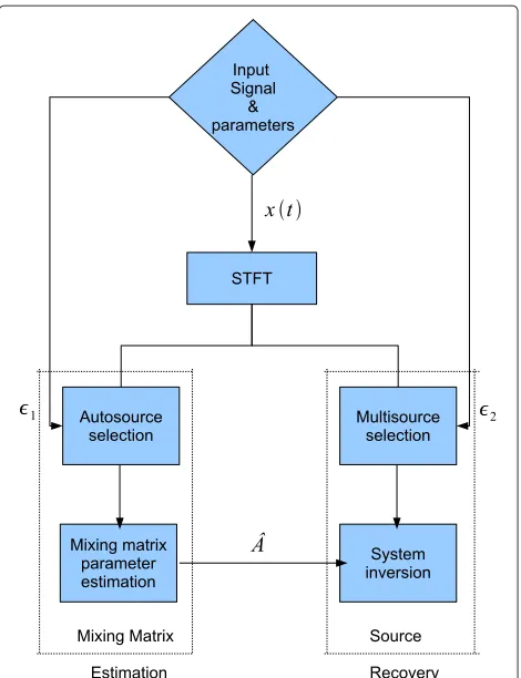
Given x(t), our purpose is to recover s(t) or equiva-lentlySs(t,f). As formalized in [28], the UBSS problem is generally decomposed in two separate subproblems. First, in the so called mixing matrix estimation, the nor-malized columns(ai)1≤i≤N are estimated so as to obtain
an estimate ofA. Then, on the basis of this estimate, the second step called signal recovery, provides a solution to Equation (2). Figure 1 presents the flowchart of such a two-step approach.
We now detail the mixing matrix estimation and the source recovery based on sparseness assumptions.
Mixing matrix estimation
The UBSS methods based on sparse signal representations in the time–frequency domain share the following main assumption:
Assumption 1. For each source, there exists a set of time– frequency points where this source exists alone.
The elements of this set can be assumed to be iso-lated time–frequency points as in degenerate unmix-ing estimation technique (DUET) [15,26] or to form a time–frequency box as in time–frequency ratio of mix-tures (TIFROM) [16] and time–frequency CORRelation (TIFCORR) [27]. Assumption 1 is often reasonable thanks to the sparseness of the time–frequency representation of the sources, especially when this number of sources is moderate.
As mentioned above, the first step in UBSS methods is to estimate the mixing matrix A to achieve source recovery. In most two-step source separation algorithms
Figure 1Flowchart of standard two-step BSS algorithms.
[12,13,15-18] an autosource selection is performed. By autosource selection, it is meant the detection of regions where only one source occurs. The methods for estimating
Aon the basis of Assumption 1 can then be summarized as follows.
Jourjine et al. [26] present the DUET method, which is restricted to two mixtures (M = 2). They address the anechoic case, where source transmission attenuations and delays between sensors are taken into account. The columns of the mixing matrix are estimated by finding picks in a 2Dhistogram of amplitude-delay estimates.
In [16], the mixing matrix estimation of the TIFROM method is based on the complex ratios SSxj(t,f)
xk(t,f), where,
given m ∈ {1, 2,. . .,M}, Sxm(t,f) stands for the mth
coordinate of Sx(t,f). These ratios are computed for each time–frequency point and for two arbitrarily chosen indicesjandk in{1, 2,. . .,M}. A first limitation of this method is to assume non-null matrix coefficients. A sec-ond limitation is the use of an empirical threshold to select the smallest empirical variances of these ratios.
The subspace-based UBSS (SUBSS) method [15] relies on another type of mixing matrix estimation. Letkstand for the set of all the time–frequency points(t,f)where the
kth source is present andstand for the union of all these setsk fork = 1, 2,. . .,N. According to Assumption 1,
the setskare non-empty and so is. For(t,f)∈k, (2)
reduces to
Sx(t,f)=Ssk(t,f)ak+Sn(t,f). (3)
According to this result, the mixing matrix can be esti-mated as follows. First, all the spatial direction vectors
d(t,f) = Sx(t,f)
Sx(t,f), with (t,f) ∈ , are clustered by
using an unsupervised clustering algorithm and taking into account that the number of sources is supposed to be known. Since (3) shows that for all the time–frequency points (t,f) of k, the STFT vectors Sx(t,f)have same spatial direction ak, the column vectors of the mixing
matrix A are then estimated as the centroids of the
N classes returned by the clustering algorithm. In [15], A¨ıssa-El-Bey et al. propose the use of thek-means algo-rithm but other techniques could be employed. The set required for the clustering procedure is determined by comparing the ratioSx(t,f)/max
ξ Sx(t,ξ )to a
thresh-old height, whose value is chosen empirically.
Source recovery
This section presents a number of techniques used in the source recovery stage of two-step UBSS algorithms. In the underdetermined case, the system (2) has less equations than unknowns, and thus it has (in general) infinitely many solutions. In order to recover the original sources, additional assumptions are needed.
The DUET method [26] assumes the sources to be (approximately) W-disjoint orthogonal in the time– frequency domain, that is, the supports of the STFTs of any two sources present in the observations are dis-joints. The source recovery is performed by partitioning the time–frequency plane using the mixing parameter estimates. This procedure assigns a source to each time– frequency point, even if this point is due to noise alone, which is detrimental to the method overall performance.
Although TIFROM and TIFCORR do not require the sources to beW-disjoint orthogonal for source recovery, they however suffer from the same limitation as DUET in that they also assign time–frequency points of noise alone to sources.
Bofill and Zibulevsky [18] use the 1-norm
minimiza-tion to recover the sources. In the noiseless case, this can be accomplished by solving the convex optimization
min Ss(t,f)
Ss(t,f)1 subject to Sx(t,f)=ASs(t,f), (4)
where·1is the1norm. In presence of noise, the
fore-going constraint must be modified so as to take the noise standard deviation into account. In practice, this noise standard deviation is unknown and must be estimated.
For the SUBSS approach in [15], the source recovery is based on the following assumptions:
Assumption 2. The number of active sources at any(t,f)
is strictly less than the number M of sensors.
Assumption 3. Any M × M sub-matrix of the mixing matrix has full rank, that is, for all J ⊂ {1, 2,. . .,N}with cardinality less than M,(aj)j∈J are linearly independent.
The subspace approach then performs multisource selection, that is, the selection of time–frequency points pertaining to a mixture and then, identifies the sources present at a multisource time–frequency points. Thanks to Assumption 2, the method then involves solving the resulting locally overdetermined linear problem. By con-struction, the methods requires rejecting time–frequency points of noise alone. In [15], the time–frequency points with energy below some empirically chosen threshold are rejected.
Statistical tests for sparseness-based UBSS
This section is the main core of the article since it is dedicated to a series of improvements brought to the clas-sical UBSS methods presented in Section “Main steps of standard UBSS methods”. These improvements concern the selection of the time–frequency points of interest for source separation (multisource selection) and the selec-tion of the time–frequency points suitable for mixing matrix estimation (autosource selection). The crux of the approach followed bellow is to consider the aforemen-tioned selections of time–frequency points as statistical testing problems of accepting or rejecting the presence of sources in noise. These two hypothesis testing problems are different in that mixing matrix estimation requires selecting points where only one single source is present, whereas this constraint is useless for denoising and source recovery.
The issue in these binary hypothesis testing prob-lems is twofold. On the one hand, the observation in each problem has unknown distribution because basi-cally the possible source signal distributions are them-selves unknown. On the other hand, the noise standard deviation is unknown as well. Because of this lack of prior knowledge, standard likelihood theory or extensions such as generalized likelihood ratios or invariance-based approaches do not apply.
a statistical test, also designed for noisy sparse signal representations.
For mixing matrix estimation, we exploit the physical nature of the signals to detect the time–frequency points where one single source is present. For signals with high overlapping rate, SNT is appropriate to select such time– frequency points. When the signals have low overlapping rate, we directly use the time–frequency points provided by the source recovery procedure.
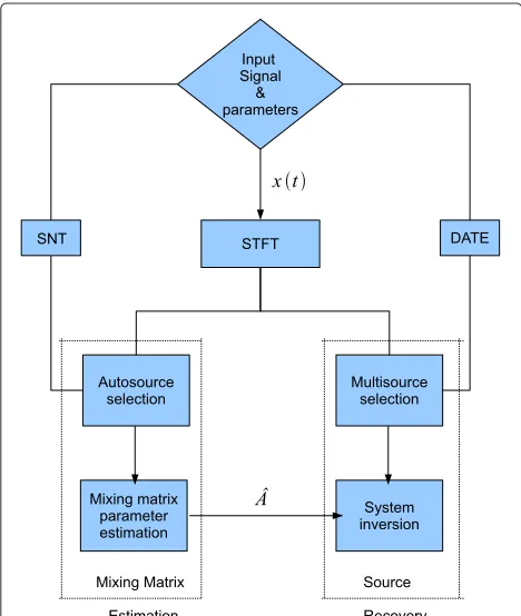
Figure 2 presents the flowchart of the proposed approach based on the DATE and SNT.
Weak-sparseness-based time–frequency detection for source recovery (multisource selection)
Recovering sources involves detecting the time– frequency points that pertain to signals. Therefore, time–frequency points due to noise alone are useless to recover sources. Detecting the time–frequency points appropriate for source recovery thus amounts to deciding whether any given time–frequency point(t,f)pertains to some signal of interest or not. It is thus natural to state this problem as the binary hypothesis testing, where the null hypothesisH0is thatSx(t,f) ∼Nc(0,σ2IM)is
com-plex Gaussian noise and the alternative hypothesisH1is
that Sx(t,f) = (t,f)+Sn(t,f)is a source mixture in
independent and additive complex Gaussian noise, where
Figure 2Flowchart of the proposed two-step BSS algorithms.
Sn(t,f)∼ Nc(0,σ2)and(t,f)stands for the mixture of
signals possibly present at time–frequency point(t,f). The issue is then the following. Although Sx(t,f) can reasonably be modeled as a random complex variable, the distribution ofSx(t,f)can hardly be known and standard likelihood theory thus becomes useless. This difficulty can however be overcome by resorting to a weak-sparseness model that can be introduced as follows.
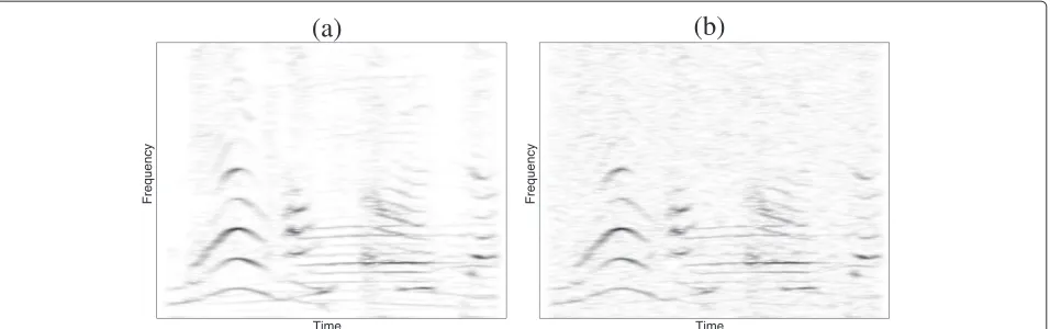
Figure 3a displays the spectrogram obtained by STFT of a mixture of audio signals. This spectrogram exhibits many time–frequency components with small or even null amplitudes. When this mixture is corrupted by additive and independent noise as in Figure 3b, small components are masked and only big ones are still visible. We must also note that the proportion of these big components remains seemingly less than or equal to one half. In other words, it is reasonable to assume that (1) the signal components are either present or absent in the time–frequency domain with a probability of presence less than or equal to one half and (2) when present, the signal components are rela-tively bigin that their amplitude is above some minimum value. These two assumptions specify the weak sparse-ness model by bounding our lack of prior knowledge on the signal distribution. The weak-sparseness model slightly differs from the “strong” sparsity model encoun-tered in compressive sensing, where it is assumed that the non-null significant signal components are very few. In the weak sparseness model, we do not restrict our attention to very small proportions of big time–frequency components.
To take the weak-sparseness model into account in our binary hypothesis problem statement, we assume that (1) the probability of occurrence of hypothesisH1is less than
or equal to one half and (2) there exists some positive real valueα such that|(t,f)| > α. The valueα can be regarded as the minimum signal amplitude. We thus write that
H0: Sx(t,f)∼Nc(0,σ2IM)
H1: Sx(t,f)=(t,f)+Sn(t,f), (5)
with Sn(t,f) ∼ Nc(0,σ2), |(t,f)| > α andP(H1)
1/2. Furthermore, we do not assume that the proba-bility distribution of (t,f) is known. In what follows, we prefer summarizing this testing problem by intro-ducing a Bernoulli distributed random variable ε(t,f), valued in{0, 1}, independent of (t,f) andSn(t,f), but
defined on the same probability space, so as to write that Sx(t,f) = ε(t,f)(t,f) + Sn(t,f). We thus have P(H1) = P[ε(t,f) = 1]. Given any test T, that is, any measurable map of CM into {0, 1}, we then say that T accepts (resp. rejects) the null hypothesis H0
Figure 3Effect of noise on sparse signals.(a)Noiseless audio signal mixture in the time–frequency domain. Many time–frequency coefficients are close to 0.(b)Noisy audio signal mixture in the time–frequency domain. The time–frequency coefficients with small amplitudes are masked by noise. Only big time–frequency coefficients remain visible. They are not really affected by noise as long as the signal to noise ratio is large enough. The proportion of these significant coefficients is less than one half.
words, T is said to return the expected value of the true hypothesis. The error probability of T is then defined as the probability Pe{T} = P[T(Sx(t,f)) = ε(t,f)].
According to ([25], Theorem VII.1), the decision should then be performed by using the thresholding test with threshold heightλD(α,σ )=(σ/
√
2)ξ(α√2/σ )where, for any positiveρ,ξ(ρ) = I−01(eρ2/2)/ρ and I0is the zeroth
order modified Bessel function of the first kind. By thresh-olding test with threshold heighth∈[ 0,∞), we mean the testThsuch that
Th(u)=
1 if|u|h
0 if|u|<h. (6)
The reasons for which this test is recommended are the following ones. Let LMPE be the minimum-probability-of-error (MPE) test, that is, the likelihood ratio test that guarantees the least possible probability of error among all possible tests and that could be computed if the prob-ability distribution of(t,f)and the prior probability of presenceP(H1)were known. Two facts follow from ([25],
Theorem VII.1). First, the error probability ofTλD(α,σ )is
above the error probability of the MPE test and less than or equal to the error probability of an explicit function
V(α√2/σ ), whose expression is useless in the sequel. Sec-ond,V(α√2/σ )is a sharp upper-bound since it is attained by the error probabilities of testsLMPEandTλD(α,σ )in the
least favorable case whereP[ε= 1]= 1/2 and(t,f) = αei(t,f)with(t,f)uniformly distributed in [ 0, 2π )and i is the imaginary unit (i2= −1). To carry out this test, we must choose an appropriate value forα and perform an estimate ofσ.
The value ofαis fixed by following the same reasoning as in [29] and considering that the minimum amplitude
of the signal to detect is the noise maximum value. More specifically, givenmrandom variablesX1,X2,. . .,Xmthat
are independent and identically distributed with Xk iid∼ N(0,σ2) for 1 k m, it is known ([30], Eqs. (9.2.1), (9.2.2), Section 9.2, p. 187) ([31], p. 454) ([32], Section 2.4.4, p. 91) that
lim
m→+∞P
λu−
σln lnm
lnm max{|Xk|, 1km}λu
=1,
whereλu=σ√2 lnmis often called the universal thresh-old [33]. The maximum amplitude of(Xk)1kmhas thus
a strong probability of being close toλu whenmis large
and the universal threshold can be regarded as the noise maximum amplitude ofmnoise samples. In our case, we haveMsensors so that each observationSx(t,f)is anM -dimensional complex vector. LetLstand for the number of time–frequency points(t,f)obtained for each sensor. We thus haveM×Ltime–frequency points(t,f)and, there-fore, 2MLrandom variables—the real and imaginary parts ofSn(t,f)—that areN(0,σ2/2). The maximum amplitude
of these 2MLGaussian independent and identically dis-tributed random variables with standard deviationσ/√2 will then be considered as the minimum signal amplitude so that we set α = σlog(2ML). The threshold height used to detect the relevant time–frequency points is then λD(σ )= √σ2ξ
2 log(2ML)
, which is henceforth called the detection threshold.
time–frequency points pertaining to the signals is large. Therefore, the noisy time–frequency points are not very few and cannot play the role of outliers with respect to the main core data distribution. In a recent article [22], a new noise standard deviation estimator called the DATE has been proposed. This estimator relies on the weak-sparseness model presented before. An exhaustive presentation of the theoretical background on which this estimator is based is beyond the scope of the present arti-cle and the reader is asked to refer to [22] for an heuristic presentation and a complete mathematical description of the DATE. In the context addressed in the present article, this algorithm applies as follows.
With the notation used so far, each Sx(t,f) is an M -dimensional complex vector. LetSxj(t,f),j=1, 2,. . .,M,
be the components of Sx(t,f). For any given j =
1, 2,. . .,M, we assume that the L time–frequency com-ponents Sxj(t,f) for thejth sensor are independent and
that each time–frequency component obeys the binary hypothesis model of (5) withα = σlog(2ML). Accord-ing to [22] and settAccord-ingκ = 2(3/2)whereis the stan-dard Gamma function, there exists a specific convergence criterion, for which we have:
(t,f)
|Sxj(t,f)|1(|Sxj(t,f)|λD(σ ))
(t,f)
1(|Sxj(t,f)|λD(σ ))
≈κσ (7)
when the numberLof time–frequency bins(t,f)is large enough. In the previous equation,1(|Sxj(t,f)| λD(σ ))
stands for the indicator function of event |Sxj(t,f)|
λD(σ ), The specific convergence criterion involved in (7)
is specified in [22] and is not given here because of its intricateness. It also turns out that the noise standard deviationσ is the unique solution of (9) with respect to the convergence criterion involved. Therefore, the DATE basically performs an estimate of the noise standard devi-ation by solving (7) with regard to this convergence cri-terion. The several steps involved in the computation are then the following ones.
The DATE:
Givenj ∈ {1, 2,. . .,M}, letY(j1),Y(j2),. . .,Y(jL) be the L
values|Sxj(t,f)|sorted by ascending order.
(1) [Search interval]:
(a) Choose some positive real valueQ less than or equal1−4(L/2L−1)2.
(b) Seth=1/√4L(1−Q)
(c) Computekmin=L/2−hL. According to
Bienaym´e–Chebyshev’s inequality and since the probabilities of presence of the signals are assumed to be less than or equal to one half, the probability that the number of
observations due to noise alone is abovekmin
is larger than or equal toQ. In the
experimental results presented below,Q was set to0.95for the computation ofkmin.
(2) [Existence]:
IF there exists a smallest integerk in
{kmin,. . .,L}such that
|Y(jk)|μj(k)/κ
ξ2 log(2ML)
<|Y(jk+1)|
(8)
with
μj(k)=
⎧ ⎨ ⎩ 1 k
k
r=1|
Y(jr)| ifk=0
0 ifk=0,
(9)
setk∗=k. ELSE, setk∗=kmin.
(3) [Value]: The estimateσj∗of the noise standard deviation on thejthsensor is then
σj=μj(k∗)/κ, (10)
The final estimateσ of the noise standard deviation is then obtained by averaging the values σj so that σ = (1/M) Mj=1σj.
Signal source detection for mixing matrix estimation (autosource selection)
In this section, we propose a test for selecting the time– frequency points where one signal source is probably present alone. To perform this selection, we make the distinction between signals with either low or high over-lapping rate in the time–frequency domain. Chirp signals (resp. audio signals) are typical examples of signals with low (resp. high) overlapping rate. It is worth noticing that the estimation procedures proposed below for each class have reasonable computational costs.
The case of signals with low overlapping rate
averaging effect inherent to any mixing matrix estimation method.
The case of signals with high overlapping rate
When signals overlap significantly in the time–frequency domain, the time–frequency detection of Section “Weak-sparseness-based time–frequency detection for source recovery (multisource selection)” is now inap-propriate. Indeed, the statistical procedure of Section “Weak-sparseness-based time–frequency detection for source recovery (multisource selection)” is aimed at detecting time–frequency points where signal sources are present, whatever the number of these sources, whereas it is now required to discriminate points where one single source is present from points where multiple sources occur. We assume that in case of different sources present at time–frequency point(t,f), they are uncorrelated and incoherently combined. The resulting energy at (t,f) is thus supposed to be smaller than the energy attained at the time–frequency points where one single source is present only.
Our purpose is thus to detect the time–frequency points where the signal energy is big enough in pres-ence of noise. Basically, this problem amounts to deciding whether|ASs(t,f)|is above some valueτor not. The value τ2thus represents the minimum energy level above which we consider that the signal energy is big enough to assume that one single source is actually present at(t,f). For any λ∈(0,∞), it follows from ([23], Lemma 4, statement (iii)) that
P|Sx(t,f)|> λ|ASs(t,f)|< τ1−Fχ2 2M(2τ2/σ2)
2λ2/σ2,
(11)
where Fχ2
d(δ)(·) stands for the cumulative distribution
function of the non-centered chi-2 distribution with d
degrees of freedom and non-centrality parameterδ. The degree of freedom in (11) is 2Msince eachSx(t,f)is an
M-dimensional complex random vector and, thus, a 2M -dimensional real random vector. Given some level γ ∈ (0, 1), it then suffices to choose
λ=λ(τ,γ )=σ
1 2F
−1
χ2
2M(2τ2/σ2)
(1−γ ). (12)
to guarantee a “false alarm probability” P|Sx(t,f)| > λ|ASs(t,f)|< τ
less than or equal toγ.
Therefore, for a given time–frequency point(t,f), the decision is that |ASs(t,f)| < τ if |Sx(t,f)| < λ(τ,γ ) and that|ASs(t,f)| τ if|Sx(t,f)| λ(τ,γ ). For mix-ing matrix estimation, we then keep the time–frequency points(t,f)such that|Sx(t,f)| λ(τ,γ ), which are con-sidered as to time–frequency points pertaining to one single source. In practice, since the actual value of σ is
unknown, we replace this true value by its estimateσ provided by the DATE.
Although the two parameters γ andτ must be fixed, there is no need to choose them for each signal to noise ratio. Parameterτ, which is independent of the noise level, can be fixed via a small noiseless database. Similarly, level γ can be determined via a few preliminary test on a small representative database.
Simulation results
In most of the following simulations, the mixing matrix is chosen according to ([14], Eq. (38)) so as to modelN
sources arriving at the sensor array at different angles θ1,θ2,. . .,θM. The entries of matrixAare thereforeaj,k = eiπ(j−1)sin(θk) forj ∈ {1,. . .,M} and k ∈ {1,. . .,N}. In
the sequel, we proceed by choosing four sources (N =4), three sensors (M= 3),θ1= 15◦,θ2= 30◦,θ3= 45◦and
θ4=75◦.
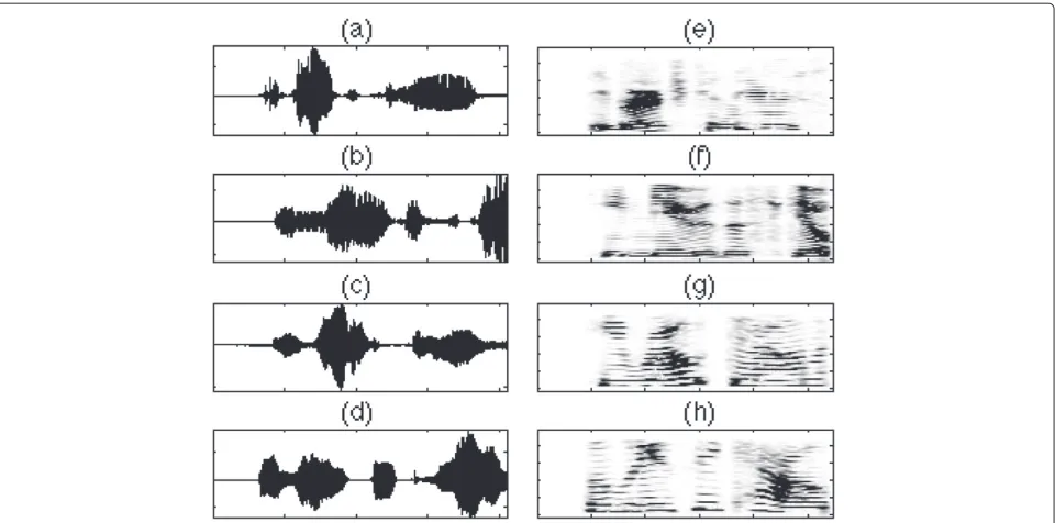
Unless specified otherwise, the source signals are speech signals randomly chosen in the TI-digits database [36]. This large speech database collected in a quiet environ-ment is commonly used in speech processing. In this article, the chosen speech signals were downsampled to 8 kHz. All signals involve 8, 192 samples. Figure 4a–d shows the time-domain representations of the original source signals and Figure 4e–h represents their corre-sponding spectrograms. Figure 5 displays a spectrogram of a mixture of these speech signals when the mixing matrixA is applied to them at SNR = 10 dB. The spec-trograms of the other mixtures are not presented because the differences between any two of them are not visu-ally noticeable since the mixing matrixAinvolves no null entry.
The two parameters required for the mixing matrix esti-mation are then fixed toτ =4 andγ =10−3. The source separation performance is measured by the normalized mean square error (NMSE):
NMSE=min
i,j ⎧ ⎨ ⎩10 log10
⎛
⎝1− sˆi,sj
sˆi·sj
2⎞
⎠ ⎫ ⎬ ⎭.
(13)
Throughout this section, NMSEs are calculated over 100 Monte-Carlo runs.
SUBSS method
Figure 4Time and time-frequency representation of speech signal.(a)–(d)show the waveforms of the original source signals in the time domain,(e)–(h)display the spectrograms of these source signals in the time–frequency domain.
The waveforms of the recovered source signals by the modified SUBSS algorithm are represented in Figure 6. Figure 6a–d shows the time-domain representations of the recovered source signals in the noiseless case (input SNR = 45 dB), and Figure 6e–h represent time-domain repre-sentations of the recovered source signals with input SNR = 10 dB.
In Figure 7, the performance of the modified SUBSS algorithm, with and without denoising, is compared to that obtained by the originally SUBSS algorithm of [15].
Mixture spectrogram
Time
Frequency
Figure 5Speech mixture spectrogram when mixing matrixAis applied to the four sources of Figure 4 (SNR = 10 dB).
The denoising mentioned above is described in Appendix as a standard linear estimation.
The modified SUBSS algorithm outperforms the orig-inal SUBSS algorithm [15], which relies on thresholds that are manually chosen for each input SNR. Moreover, modified SUBSS without denoising yields performance measurements that do not significantly depart from those attained by the original subspace-based UBSS algorithm. In addition, Figure 7 displays the NMSEs obtained by using the MAD estimator instead of the DATE in the mod-ified SUBSS algorithm without denoising. The use of the MAD instead of the DATE induces a significant perfor-mance loss, which illustrates the relevance of the DATE and the weak-sparseness model. In Figures 8 and 9, we present the NMSEs obtained by the modified SUBSS and the original SUBSS when the number of sources increases and for SNR = 10dB and SNR = 20dB. In both figures, the NMSEs degrade, because an increase of the source interference invalidates Assumption 1.
We now consider the case of complex chirp signals. These ones were generated by slightly modifying theMAT
-L AB routineMakeSignal.m of theWAVEL AB toolbox, so as to obtain complex chirp signals. The 4 chirp signals we use as sources ares1(t) = √t(1−t)ei
πT
2 t2, s2(t) = √
t(1−t)e−iπ4Tt2, s3(t) = e−iπTt2 and s4(t) = ei
Figure 6Simulation results:(a)–(d)show the waveforms of the source signals recovered by modified SUBSS with input SNR = 45 dB, (e)–(h)show the waveforms of the source signals recovered by modified SUBSS with input SNR = 10 dB.
of these sources when matrix A is applied and SNR = 10 dB. The spectrograms of the other mixtures are not dis-played for the same reasons as those given previously for the speech signal mixtures.
The experimental procedure for assessing the modi-fied SUBSS in comparison to the original SUBSS method is then the same as above. As specified in Section “The case of signals with low overlapping rate”, the thresholds used for the mixing matrix estimation are the detec-tion ones. Therefore, no addidetec-tional parameter is needed.
0 5 10 15 20 25 30 35 40
−18 −16 −14 −12 −10 −8 −6 −4 −2
SNR (dB)
NMSE (dB)
SUBSS
MAD Modified SUBSS without denoising Modified SUBSS without denoising Modified SUBSS with denoising
Figure 7Comparison between SUBSS, modified SUBSS with and without denoising, modified SUBSS with MAD estimate instead of DATE and without denoising: NMSE versus SNR.
The results obtained in Figure 12 show the relevance of this choice for the thresholds, explained by the fact that chirp signals present very few overlapping time– frequency components.
Other methods
As described in Sections “Weak-sparseness-based time–frequency detection for source recovery (multi-source selection)” and “Signal (multi-source detection for mixing matrix estimation (autosource selection)”, The DATE and
4 4.5 5 5.5 6 6.5 7 7.5 8
−8 −7 −6 −5 −4 −3 −2 −1 0
Number of sources
NMSE (dB)
SUBSS
Modified SUBSS without denoising
4 4.5 5 5.5 6 6.5 7 7.5 8 −12
−10 −8 −6 −4 −2 0
Number of sources
NMSE (dB)
SUBSS
Modified SUBSS without denoising
Figure 9Comparison between SUBSS and modified SUBSS without denoising when input SNR = 20 dB: NMSE versus number of sources.
SNT can be used to perform multisource and autosource selections, respectively. Said otherwise, the statistical tests of the aforementioned sections make it possible to obtain the time–frequency points where noisy mixtures are present and the set of time–frequency points where only one single source exists. In this section, we comment the results we obtain by so proceeding with respect to the several UBSS methods addressed in Section “Main steps of standard UBSS methods” and other than SUBSS.
(a)
Time
Frequency
Figure 11Chirp signal mixture spectrogram when mixing matrix Ais applied to the chirp signals of Figure 10 (SNR = 10 dB).
In the underdetermined case, TIFROM achieves partial source separation only. Therefore, to better assess the con-tribution of our statistical tests to TIFROM, we consider the determined case where four source signals from four speakers are mixed. The mixing matrix is now 4×4 with independent Gaussian entries. In Figure 13, we present the NMSEs obtained by the TIFROM, SNT-TIFROM and Modified SNT-TIFROM. Specifically, SNT-TIFROM uses SNT to select times frequency points where a source
(a)
Time
Frequency
(b)
Time
Frequency
(c)
Time
Frequency
(d)
Time
Frequency
0 5 10 15 20 25 30 35 40 −25
−20 −15 −10 −5 0
SNR (dB)
NMSE (dB)
SUBSS
Modified SUBSS without denoising
Figure 12Comparison of performance between SUBSS and modified SUBSS without denoising for chirp signals: NMSE versus SNR.
exists alone. SNT-TIFROM, as TIFROM, performs no multisource selection for source recovery. In contrast, the modified SNT-TIFROM performs multisource selection and forces to zero the unselected time–frequency points. These results show that SNT makes it possible to actu-ally select the autosource time–frequency points, with no performance loss and without resorting to the empirical threshold required by the original TIFROM. The per-formance yielded by the modified SNT-TIFROM further emphasizes that the detection threshold adjusted with the DATE selects appropriate multisource time–frequency points for source recovery. The gain for low SNRs is explained by the fact that this selection can be regarded as a non-linear denoising. The gain brought by this denoising effect decays when the SNR increases.
Figure 13Comparison of performance between TIFROM, SNT-TIFROM and Modified TIFROM: NMSE versus SNR.
Another contribution of our statistical approach to sparseness-based methods is the estimation of the noise standard deviation. Indeed, some methods need an esti-mate or the true value of the noise standard deviation. For instance, Bofill and Zibulevsky [18], use the1-norm
min-imization to recover the sources. In the noisy case, they propose to solve the optimization problem:
min Ss(t,f)
1
2σ2Sx(t,f)−ASs(t,f) 2
2+Ss(t,f)1.
Because of the weakly sparseness of the sources in noise, we hereafter prefer following [37] dedicated to stable recovery of not exactly sparse signals. We therefore solve the optimization problem
min Ss(t,f)
Ss(t,f)1 subject to Sx(t,f)−ASs(t,f)2
≤σ2(M+2√2M). (14)
This approach can then be improved in two ways. First, by solving this optimization problem on only the time–frequency points selected by the multisource pro-cedure propounded in Section “Weak-sparseness-based time–frequency detection for source recovery (multi-source selection)”. Second, by replacing the unknown true value of the noise standard deviation by its estimate pro-vided by the DATE. In this respect, Figure 14 displays the performance measurements obtained by the original method based on the1-criterion of Equation (4) (L1
Min-imization) in comparison to the modified1-criterion of
0 5 10 15 20 25 30 35
−18 −16 −14 −12 −10 −8 −6 −4 −2 0
SNR (dB)
NMSE (dB)
L1 Minimization Modified L1 Minimization MAD Modified L1 Minimization Oracle Modified L1 Minimization
Figure 14Comparison of performance (NMSE versus SNR) between the original Bofill and Zibulevsky’s method based on the1-criterion of Equation (4) (L1 Minimization), the modified
Equation (14) applied to the outcome of the the mul-tisource selection when the noise standard deviation is estimated by the DATE (Modified L1 minimization). As expected, the gain brought by multisource selection and Equation (14), both adjusted by the noise standard devi-ation estimate provided by the DATE, is significant. It is also worth noticing that the DATE estimation error does not impact significantly the separation performance in comparison to the case where the noise standard devia-tion is perfectly known. This can also be seen in Figure 14, where the performance measurements are given when the multisoure selection and1-criterion of Equation (14) are both adjusted with the actual value of the noise standard deviation (Oracle Modified L1 Minimization). In contrast, there is significant performance loss when the multisource selection and Equation (4) are calculated by using the MAD instead of the DATE (MAD Modified L1 Minimiza-tion). The reason still relates to the fact that the DATE is more robust to weak-sparseness than the MAD.
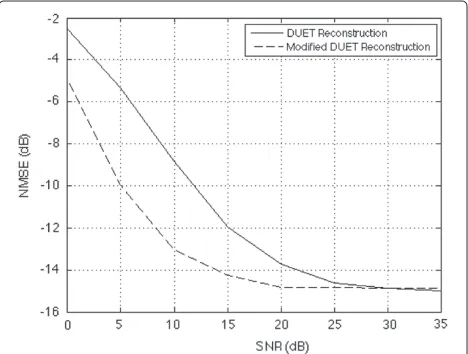
The multisource selection based on the detection threshold adjusted by the estimate provided by the DATE can be further exploited by the DUET reconstruction, as illustrated in Figure 15. In this simulation, the input sig-nals are the chirp sigsig-nals considered above, so that the
W-disjoint orthogonality assumption is satisfied. More-over, the mixing matrixAis now assumed to be known. On the one hand, we perform the DUET source recov-ery by considering the whole time–frequency plane. On the other hand, we consider the modified DUET, that is, the DUET source recovery applied to the selected multi-source time–frequency points only. The results are similar to those obtained above by TIFROM and its modified versions. Here, the gain brought by the multisource selec-tion, which acts as a denoising, is bigger on a wider SNR
Figure 15Comparison of performance between DUET reconstruction and modified DUET reconstruction on chirp signals.
range because the time–frequency representation of chirp signals is sparser than that of audio signals.
Discussion Assessment
The algorithms we propose are very general. They are not dedicated to a given sparseness-based BSS method. They are simple to apply without any adjustment. From the results of Section “Simulation results”, our procedures can therefore be used to improve, simplify or bring robustness to the standard sparseness-based BSS methods considered in the article.
More specifically, the weak-sparseness-based time– frequency detection procedure of Section “Weak-sparse-ness-based time–frequency detection for source recovery (multisource selection)” can be used as an automatized pre-processing for multisource selection. For example, the time–frequency detection in [15] requires one threshold value for each instrumented SNR. The detection proce-dure of Section “Weak-sparseness-based time–frequency detection for source recovery (multisource selection)” then makes it possible to avoid this empirical parameter choice, which brings robustness and significant simplifi-cation. Used as a pre-processing for TIFROM [16], which basically involves no selection of time–frequency points, the multisource selection we propound can improve the separation performance.
For mixing matrix estimation, our approach described in Section “Signal source detection for mixing matrix estimation (autosource selection)” relies on no weak-sparseness assumption and involves two parameters only, that is, the tolerance and the false-alarm probability. These parameters are valid over the signal-to-noise ratio (SNR) range, in contrast to [15] for instance. Furthermore, the assumptions made by TIFROM can be relaxed by using the autosource selection of Section “Signal source detec-tion for mixing matrix estimadetec-tion (autosource selecdetec-tion)”. It is also worth noticing that the two parameters we need for mixing matrix estimation have a physical meaning, which is not the case for some standard sparseness-based BSS methods.
Convolutive mixture case
instance, this detection procedure for multisource selec-tion can be used straightforwardly to detect the time– frequency points required by the convolutive SUBSS pre-sented in [38]. The modified convolutive SUBSS thus obtained discards the empirical threshold required in [38] for multisource selection. This entails no significant per-formance loss, as illustrated by Figure 16. Studying the added-value brought by SNT in the convolutive mixture case requires further analysis that could be achieved in some forthcoming work.
Conclusion and perspectives
The algorithms presented in this article contribute to BSS in the underdetermined mixture case, by avoiding empir-ical choices of parameters present for the so-called family of weak-sparseness based methods. Our first algorithm aimed at selecting the suitable time–frequency points for source recovery is full automatic. The second, ded-icated to mixing matrix estimation, requires fixing two parameters only, regardless of the instrumented SNRs.
The question is now to what extent the statistical tests used above in the instantaneous mixture case can possibly be exploited in the convolutive mixture case, especially in complement to the results discussed in Section “Convolu-tive mixture case”. It can also be wondered whether these tests can be extended so as to deal with colored noise. Work on this topic is under progress.
The theoretical and experimental results of this article pinpoint that the subfunctions of the source separation methods considered above, completed with the statistical tests we have proposed, can be regarded as elementary components that can be interchanged and associated to
0 5 10 15 20 25 30 35
−15 −10 −5 0
SNR (dB)
NMSE (dB)
Convolutive SUBSS Modified Convolutive SUBSS
Figure 16Comparison of performance between standard convolutive SUBSS and modified convolutive SUBSS: the signals used are same audio one as those considered in simulation section.Each mixture is a sum of filtered source signal where each filter is randomly chosen RIF with order 4.
provide new algorithms for source separation in different applicative contexts. This opens new practical prospects. For instance, it would be desirable to construct a tool-box involving all these elementary components for further developments and studies. Such a toolbox would also make it possible to carry out exhaustive experimental assessments on large databases of signals via the BSSEval toolbox, downloadable from [39].
Appendix
Denoising-based source recovery
The SUBSS method presented in [15] estimates the index set of the sources present at a given time–frequency point (t,f). Let us denote byJthis set of indexes. Then, Equation (2) reduces to:
Sx(t,f)=AJSsJ(t,f)+Sn(t,f) (15)
and the STFT coefficients of these active sources can be recovered using:
SsJ(t,f)≈A#JSx(t,f), (16)
where A#J = (AHJ AJ)−1AHJ is the Moore-Penrose
pseu-doinverse ofAJ.
We propose to use the noise standard deviation estimate provided by the DATE to jointly denoise and separate the sources on the basis of the time–frequency points selected by the statistical test of Section “Weak-sparse-ness-based time–frequency detection for source recovery (multisource selection)”. So, instead of performing the source separation as specified by Equation (16), the source separation is now carried out by computing
SsJ(t,f)=RsJA
H
J (AJRsJA
H
J +σ2IM)−1Sx(t,f) (17)
whereσ is the noise standard estimate returned by the DATE andRsJ = E[SsJ(t,f)SsHJ(t,f)]. The derivation of
the optimal linear estimator of (17) is standard. It involves minimizing the riskESsJ(t,f)−DSx(t,f)
2
whenD
ranges over the space of the card(J)× Mmatrices and under the assumption that the sources are spatially decor-related. In practice, matrix RsJ is unknown and must be
estimated. We then proceeded as follows. On the one hand, we haveRx= ARsAH+σ2IM. On the other hand,
Rx can be estimated by !Rx = #t1 tSx(t,f)Sx(t,f)H, where #tstands for the number of time windows on which the STFT is calculated. Since estimates of A and σ are known, we derive from the expressions ofRx and!Rxan estimateRsofRs. An estimate ofRsJfollows by picking the
Competing interests
The authors declare that they have no competing interests.
Received: 14 July 2011 Accepted: 1 July 2012 Published: 16 August 2012
References
1. V Varajarajan, J Krolik, Multichannel system identification methods for sensor array calibration in uncertain multipath environments. inIEEE Signal Processing Workshop on Statistical Signal Processing (SSP)(Singapore, Oct 2001), pp. 297–300
2. A Rouxel, DL Guennec, O Macchi, Unsupervised adaptive separation of impulse signals applied to EEG analysis. inIEEE International Conference on Acoustics, Speech, Signal Processing (ICASSP),vol. 1 (Istanbul, Turkey, June 2000), pp. 420–423
3. K Abed-Meraim, S Attallah, T Lim, M Damen, A blind interference canceller in DS-CDMA. inIEEE International Symposium on Spread Spectrum Techniques and Applications(Parsippany, Sept 2000), pp. 358–362 4. I Dur´an-D´ıaz, SA Cruces-Alvarez, A joint optimization criterion for blind
DS-CDMA detection. EURASIP J. Adv. Signal Process.2007(79248), 1–11 (2007)
5. A A¨ıssa-El-Bey, K Abed-Meraim, Y Grenier, Underdetermined blind audio source separation using modal decomposition. EURASIP J. Audio Speech Music Process.2007(85438), 1–15 (2007)
6. P Comon, C Jutten (eds.),Handbook of Blind Source Separation: Independent Component Analysis and Blind Deconvolution(Academic Press, Oxford, 2010)
7. J-F Cardoso, Blind signal separation: statistical principles. Proc. IEEE. 86(10), 2009–2025 (1998)
8. A Belouchrani, K Abed-Meraim, J-F Cardoso, E Moulines, A blind source separation technique using second-order statistics. IEEE Trans. Signal Process.45(2), 434–444 (1997)
9. A Belouchrani, MG Amin, Blind source separation based on
time-frequency signal representations. IEEE Trans. Signal Process.46(11), 2888–2897 (1998)
10. K Abed-Meraim, Y Xiang, JH Manton, Y Hua, Blind source separation using second order cyclostationary statistics. IEEE Trans. Signal Process.49(4), 694–701 (2001)
11. AP Dempster, NM Laird, DB Rubin, Maximum likelihood from incompletes data via the EM algorithm. J. R. Stat. Soc. Ser. B.39(1), 1–38 (1977) 12. O Yilmaz, S Rickard, Blind separation of speech mixtures via
time-frequency masking. IEEE Trans. Signal Process.52(7), 1830–1847 (2004)
13. T Melia, S Rickard, Underdetermined blind source separation in echoic environments using DESPRIT. EURASIP J. Adv. Signal Process. 2007(86484), 1–19 (2007)
14. N Linh-Trung, A Belouchrani, K Abed-Meraim, B Boashash, Separating more sources than sensors using time-frequency distributions. EURASIP J. Appl. Signal Process.2005(17), 2828–2847 (2005)
15. A A¨ıssa-El-Bey, N Linh-Trung, K Abed-Meraim, A Belouchrani, Y Grenier, Underdetermined blind separation of nondisjoint sources in the time-frequency domain. IEEE Trans. Signal Process.55(3), 897–907 (2007) 16. F Abrard, Y Deville, A time-frequency blind signal separation method
applicable to underdetermined mixtures of dependent sources. Signal Process.85(7), 1389–1403 (2005)
17. S Arberet, R Gribonval, F Bimbot, A robust method to count and locate audio sources in a multichannel underdetermined mixture. IEEE Trans. Signal Process.58(1), 121–133 (2010)
18. P Bofill, M Zibulevsky, Underdetermined blind source separation using sparse representations. Signal Process.81(11), 2353–2362 (2001) 19. S Araki, H Sawada, R Mukai, S Makino, Underdetermined blind sparse
source separation for arbitrarily arranged multiple sensors. Signal Process. 87(8), 1833–1847 (2007)
20. S Araki, T Nakatani, H Sawada, S Makino, Stereo source separation and source counting with MAP estimation with dirichlet prior considering spatial aliasing problem. inIndependent Component Analysis and Signal Separation (ICA),ser. LNCS, vol. 5441 (Springer, Paraty, 2009), pp. 742–750 21. P O’Grady, B Pearlmutter, S Rickard, Survey of sparse and non-sparse
methods in source separation. Int. J. Imag. Syst. Technol.15(1), 18–33 (2005)
22. D Pastor, F-X Socheleau, Robust estimation of noise standard deviation in presence of signals with unknown distributions and occurrences. IEEE Trans. Signal Process.60(4), 1545–1555 (2012)
23. D Pastor, Signal norm testing in additive and independant standard Gaussian noise, Institut Mines-T ´el´ecom; T´el´ecom Bretagne, UEB , Lab-STICC UMR CNRS 3192, Tech. Rep., 2011, available at http://www. telecom-bretagne.eu/publications/publication.php?idpublication=10706 24. SM Aziz-Sba¨ı, A A¨ıssa-El-Bey, D Pastor, Robust underdetermined blind
audio source separation of sparse signals in the time-frequency domain. inIEEE International Conference on Acoustics, Speech and Signal Processing (ICASSP)(Prague, Czech Republic, May 2011), pp. 3716–3719
25. D Pastor, R Gay, A Gronenboom, A sharp upper bound for the probability of error of likelihood ratio test for detecting signals in white gaussian noise. IEEE Trans. Inf. Theory.48(1), 228–238 (2002)
26. A Jourjine, S Rickard, O Yilmaz, Blind separation of disjoint orthogonal signals: demixing N sources from 2 mixtures. inIEEE International Conference on Acoustics, Speech and Signal Processing (ICASSP),vol. 5 (Istanbul, Turkey, June 2000), pp. 2985–2988
27. Y Deville, M Puigt, Temporal and time-frequency correlation-based blind source separation methods. part I: determined and underdetermined linear instantaneous mixtures. Signal Process.87(3), 374–407 (2007) 28. F Theis, E Lang, Formalization of the two-step approach to overcomplete
BSS. inSignal and Image Processing (SIP)(Kauai, USA, August 2002), pp. 207–212
29. AM Atto, D Pastor, G Mercier, Detection thresholds for non-parametric estimation. Signal Image Video Process.2(3), 207–223 (2008) 30. SM Berman,Sojourns and Extremes of Stochastic Processes(Wadsworth,
Reading, MA, 1992)
31. S Mallat,A Wavelet Tour of Signal Processing,2nd (Academic Press, Cambridge, 1999)
32. RJ Serfling,Approximations Theorems of Mathematical Statistics(Wiley, New York, 1980)
33. DL Donoho, IM Johnstone, Ideal spatial adaptation by wavelet shrinkage. Biometrika.81(3), 425–455 (1994)
34. F Hampel, The influence curve and its role in robust estimation. J. Am. Stat. Assoc.69(346), 383–393 (1974)
35. P Huber, E Ronchetti,Robust Statistics,2nd edn. (Wiley, New York, 2009) 36. R Leonard, A database for speaker-independent digit recognition. inIEEE
International Conference on Acoustics, Speech, Signal Processing (ICASSP), vol. 9 (San Diego, California, USA, March 1984), pp. 328–331
37. JREJ Cand`es, T Tao, Stable signal recovery from incomplete and inaccurate measurements. Commun. Pure Appl. Math.59(8), 1207–1223 (2006) 38. A A¨ıssa-El-Bey, K Abed-Meraim, Y Grenier, Blind separation of
underdetermined convolutive mixtures using their time-frequency representation. IEEE Trans. Audio Speech Lang. Process.15(5), 1540–1550 (2007)
39. C F´evotte, R Gribonval, E Vincent, A toolbox for performance measurement in (blind) source separation, available at http://bass-db. gforge.inria.fr/bss eval/
doi:10.1186/1687-6180-2012-169