Separation of phase-locked sources in pseudo-real MEG data

(1)

R E S E A R C H

Open Access

Separation of phase-locked sources in

pseudo-real MEG data

Miguel Almeida

1*

, Jos´e Bioucas-Dias

1

and Ricardo Vig´ario

2

Abstract

This article addresses the blind separation of linear mixtures of synchronous signals (i.e., signals with locked phases), which is a relevant problem, e.g., in the analysis of electrophysiological signals of the brain such as the

electroencephalogram and the magnetoencephalogram (MEG). Popular separation techniques such as independent component analysis are not adequate for phase-locked signals, because such signals have strong mutual

dependency. Aiming at unmixing this class of signals, we have recently introduced the independent phase analysis (IPA) algorithm, which can be used to separate synchronous sources. Here, we apply IPA to pseudo-real MEG data. The results show that this algorithm is able to separate phase-locked MEG sources in situations where the phase jitter (i.e., the deviation from the perfectly synchronized case) is moderate. This represents a signiﬁcant step towards performing phase-based source separation on real data.

1 Introduction

In recent years, the interest of the scientiﬁc community in synchrony has risen. This interest is both in its phys-ical manifestations and in the development of a theory unifying and describing those manifestations in various systems such as laser beams, astrophysical objects, and brain neurons [1].

It is believed that synchrony plays a relevant role in the way diﬀerent parts of the human brain interact. For exam-ple, when humans engage in a motor task, several brain regions oscillate coherently [2,3]. Also, several pathologies such as autism, Alzheimer, and Parkinson are associated with a disruption in the synchronization proﬁle of the brain, whereas epilepsy is associated with an anomalous increase in synchrony (see [4] for a review).

To perform inference on the synchrony of networks present in the brain or in other real-world systems, one must have access to the phase dynamics of the individual oscillators (which we will call “sources”). Unfortunately, in brain electrophysiological signals such as encephalograms (EEG) and magnetoencephalograms (MEG), and in other real-world situations, individual oscillator signals are not directly measurable, and one has only access to a super-position of the sourcesa. In fact, EEG and MEG signals

*Correspondence: [email protected]

1Instituto de Telecomunicacoes, Lisbon, Portugal

Full list of author information is available at the end of the article

measured in one sensor contain components coming from several brain regions [5]. In this case, spurious synchrony may occur, as we will illustrate later.

The problem of undoing this superposition is called blind source separation (BSS). Typically, one assumes that the mixing is linear and instantaneous, which is a valid approximation in brain signals [6]. One must also make some assumptions on the sources, such as in indepen-dent component analysis (ICA) where the assumption is mutual statistical independence of the sources [7]. ICA has seen multiple applications in EEG and MEG pro-cessing (for recent applications see, e.g., [8,9]). Diﬀerent BSS approaches use criteria other than statistical indepen-dence, such as non-negativity of sources [10,11] or time-dependent frequency spectrum criteria [12,13]. In our case, independence of the sources is not a valid assump-tion, because phase-locked sources are highly mutually dependent. Also, phase-locking is not equivalent to fre-quency coherence: in fact, two signals may have a severe overlap between their frequency spectra but still exhibit low or no phase synchrony at all [14]. In this article, we address the problem of how to separate such phase-locked sources using a phase-speciﬁc criterion.

Recently, we have presented a two-stage algorithm called independent phase analysis (IPA) which performed very well in noiseless simulated data [15] and with mod-erate levels of added Gaussian white noise [14]. The

(2)

cal foundations of the algorithm and applying it to a toy dataset of manually generated data. However, in that arti-cle we were not concerned with the application of IPA to real-world data. In this article, we study the applica-bility of IPA to pseudo-real MEG data. These data are not yet meant to allow inference about the human brain; however, they are generated in such a way that both the sources and the mixing process mimic what actually hap-pens in the human brain. The advantage of using such pseudo-real data is that the true solution is known, thus allowing a quantitative assessment of the performance of the algorithm. We also study the robustness of IPA to the case where the sources are not perfectly phase-locked. It should however be reinforced that the algorithm pre-sented here makes no assumptions that are speciﬁc of brain signals, and should work in any situation where phase-locked sources are mixed approximately linearly and noise levels are low.

This article is organized as follows. In Section 2, we introduce the Hilbert transform. We also introduce there the phase locking factor (PLF), a measurement of syn-chrony which is central to the algorithm; ﬁnally, we show that synchrony is disrupted when the sources undergo a linear mixing. Section 3 describes the IPA algorithm in detail, including illustrations using a toy dataset. In Section 4, we explain how the pseudo-real MEG data are generated and show the results obtained by IPA on those data. These results are discussed in Section 5 and conclusions are drawn in Section 6.

2 Background

2.1 Hilbert transform: phase of a real-valued signal Usually, the signals under study are real-valued discrete signals. To obtain the phase of a real signal, one can use a complex Morlet (or Gabor) wavelet transform, which can be seen as a bank of bandpass filters [17]. Alterna-tively, one can use the Hilbert transform, which should be applied to a locally narrowband signal or be pre-ceded by appropriate filtering [18] for the meaning of the phase extracted by the Hilbert transform to be clear. The two transforms have been shown to be equivalent for the study of brain signals [19], but they may differ for other kinds of signals. In this article, we chose to use the Hilbert transform. To ensure that this transform yields meaningful results, we will precede its use by band-pass filtering the pseudo-real MEG sources used in this arti-cle (see Section 4.1). Note that this is a very common preprocessing step in the analysis of real MEG signals (cf., [20-22]).

xh(t)≡x(t)∗h(t), whereh(t)≡ ⎨ ⎩ 2

πt, for oddt.

Note that the Hilbert transform is a linear operator. The Hilbert ﬁlterh(t) is not causal and has inﬁnite duration, which makes direct implementation of the above formula impossible. In practice, the Hilbert transform is usually computed in the frequency domain, where the above convolution becomes a product of the discrete Fourier transforms ofx(t) andh(t). A more thorough mathemat-ical explanation of this transform is given in [18,23]. We used the Hilbert transform as implemented by MATLAB. The analytic signal ofx(t), denoted byx˜(t), is given by ˜

x(t) ≡ x(t) +ixh(t), where i = √

−1 is the imaginary unit. The phase ofx(t) is deﬁned as the angle of its ana-lytic signal. In the remainder of the article, we drop the tilde notation; it should be clear from the context whether the signals under consideration are the real signals or the corresponding analytic signals.

2.2 Phase-locked sources

Throughout this article, we assume that the sought sources, in number ofNand denoted bysj,j= 1,. . .,N,

are phase-locked. In other words,sj,j=1,. . .,Nare

com-plex valued signals with nonnegative amplitudes and equal phase up to a constant plus small perturbations. Formally,

sj(t)=aj(t)ei(αj+φ(t)+δj(t)), (1)

whereaj(t)are the amplitudes of the sources, which are

by deﬁnition non-negative and real-valued.αjis the

con-stant dephasing (or phase lag) between the sources (it does not depend on the timet),φ (t)represents an oscillation common to all the sources (it does not depend on the source j), and δj(t) is the phase jitter, which represents

the deviation of the jth source from its nominal phase

αj+φ (t). Throughout this article, we will assume that the

phase jitter is Gaussian with zero mean and a standard deviationσ.

(3)

oscillators’ phases only, not their amplitudes. The phase of oscillatorjis governed by [1,25,26]

˙

φj(t)=ωj(t)+

1 N

N

k=1

κ_jksinφ_k(t)−φj(t), (2)

whereφj(t)is the phase of oscillatorj(it is unrelated to φ (t)in Equation (1)),ωj(t)is its natural frequency, andκjk

measures the strength of the interaction between oscil-lators j and k. If the κ_jk coeﬃcients are large enough andωj(t) = ωk(t) for allj,k, then the solutions of the

Kuramoto model are of the form (1) with smallδj(t).

2.3 PLF

Given two oscillators with phasesφj(t)andφk(t)fort=1, . . .,T, the real-valuedb PLF, or phase locking value, between those two oscillators is deﬁned as

jk ≡

1 T

T

t=1

ei[φj(t)−φk(t)]

=ei(φj−φk), (3)

where·is the time average operator. The PLF satisﬁes 0≤ jk ≤1. The value jk = 1 corresponds to two

oscil-lators that are fully synchronized (i.e., their phase lag is constant). In terms of Equation (1), a PLF of 1 is obtained only if the phase jitterδj(t)is zero. The value jk = 0 is

attained, for example, if the phase diﬀerenceφj(t)−φk(t)

modulo 2π is uniformly distributed in [−π,π[. Values between 0 and 1 represent partial synchrony; in general, higher values of the standard deviation of the phase jitter

δ_j(t)yield lower PLF values.

Note that a PLF of 1 is obtained if and only ifφ_j(t)−φ_k(t)

is constantc. Thus, studying the separation of sources with constant phase lags can equivalently become the study of separation of sources with pairwise PLFs of 1.

Throughout this article, phase synchrony is measured using the PLF; two signals are perfectly synchronous if and only if they a PLF of 1. Other approaches exist, e.g., for chaotic systems or specific types of oscillators [27]. Studying separation algorithms based on such other defi-nitions is outside of the scope of this article. The definition used here has the advantages of being tractable from an algorithmic point of view, and of being applicable to any situation whereφj(t)−φk(t)is constantd, regardless of the

type of oscillator.

2.4 Eﬀect of linear mixing on synchrony

Assume that we haveNsources which have PLFs of 1 with each other. Lets(t), fort=1,. . .,T, denote the vector of sources andx(t)=As(t)denote the mixed signals, where

Ais the mixing matrix, which is assumed to be square

and non-singulare. Our goal is to ﬁnd a square unmix-ing matrix W such that the estimated sources y(t) = WTx(t) = WTAs(t) are as close to the true sources as possible, up to permutation, scaling, and sign change.

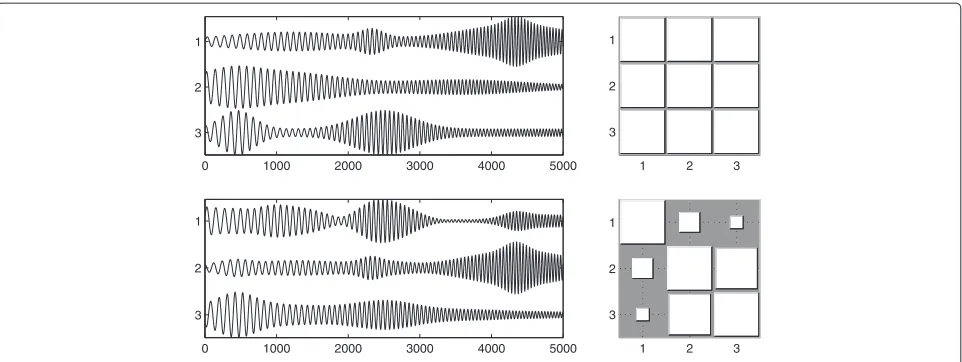
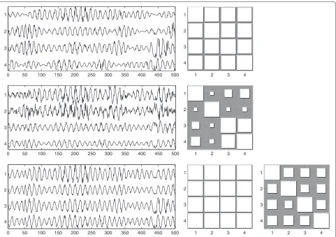
The eﬀect of linear mixing on the PLF matrix is illus-trated in Figure 1 for a set of simulated sources. This set has three sources, with PLFs of 1 with each other. These sources are of the form (1) with negligible phase jitter, and the phase lagsαjare 0,π₆, andπ₃ radians, respectively. The

common oscillation is a time-dependent sinusoid. The amplitudes are generated by adding a small constant base-line to a random number of “bursts” with Gaussian shape. Each “burst” has a random center and a random width, and each source amplitude has 1 to 5 such “bursts”.

The ﬁrst row of Figure 1 shows on the left the original sources and on the right their PLF matrix. The second row depicts the mixed signalsx(t)on the left and their PLFs on the right; the mixing matrix has random entries uni-formly distributed between−1 and 1. It is clear that the mixed signals have lower pairwise PLFs than the sources, although signals 2 and 3 still exhibit a rather high mutual PLF. This example suggests that linear mixing of syn-chronous sources reduces their synchrony, a fact that will be proved in Section 3.3, ahead; this fact will be used to extract the sources from the mixtures by trying to maximize the PLF of the estimated sources.

3 Algorithm

In this section, we describe the IPA algorithm. As men-tioned in Section 1, this algorithm ﬁrst performs subspace separation, and then performs separation within each sub-space. In this article, we only study the performance of IPA in the case where all the sources are phase-locked; in this situation, the inter-subspace separation can entirely be skipped, since there is only one subspace of locked sources. Therefore, we will not discuss here the part of IPA relating to subspace separation; the reader is referred to [14] for a discussion on that subject.

3.1 Preprocessing 3.1.1 Whitening

As happens in ICA and other source separation tech-niques, whitening is a useful preprocessing step for IPA. Whitening, or sphering, is a procedure that linearly transforms the data so that the transformed data have the identity as its covariance matrix; in particular, the whitened data are uncorrelated [7]. In ICA, there are clear reasons to pursue uncorrelatedness: independent data are also uncorrelated, and therefore whitening the data already fulﬁlls one of the required conditions to ﬁnd

independent sources. If D denotes the diagonal matrix

containing the eigenvalues of the covariance matrix of

the data and V denotes an orthonormal matrix which

has, in its columns, the corresponding eigenvectors, then whitening can be performed in a PCA-like manner by multiplying the datax(t)by a matrixB, where [7]

(4)

1 2 3 3

0 1000 2000 3000 4000 5000

3 2 1

1 2 3

1

2

3

0 1000 2000 3000 4000 5000

3

Figure 1Top row: The three original sources (left) and PLFs between them (right).Bottom row: The three mixed signals (left) and PLFs between them (right). On the right column, the area of the square in position(i,j)is proportional to the PLF between the signalsiandj. Therefore, large squares represent PLFs close to 1, while small squares represent values close to zero. In this example, the second and third sources have phase lags ofπ

6 and π

3 radians relative to the ﬁrst source, respectively.

The whitened data are given byz(t)=BAs(t). Therefore, whitening merely transforms the original source

separa-tion problem with mixing matrixAinto a new problem

with mixing matrixBA. The advantage is thatBAis an orthogonal mixing matrix, and its estimation becomes easier [7].

The above reasoning is not valid for the separation of phase-locked sources. However, under rather general assumptions, satisﬁed by the data studied here, it can be shown that whitening places a relatively low upper bound on the condition number of the equivalent mixing matrix (see [28] and references therein). Therefore, we always whiten the mixture data before applying the procedures described in Section 3.2.

3.1.2 Number of sources

As will be seen below, IPA assumes knowledge of the num-ber of sources, and also assumes that the mixing matrix is square: if this is not the case, a simple procedure can be used to detect the number of sources and to transform the data to obey these constraints. If the mixing process is noiseless and is given byx(t)=As(t), whereAhas more

rows than columns and has maximum rankf_{, the number}

of non-zero eigenvalues of the covariance matrix of xis N, whereNis the number of sources (or equivalently, the number of columns of A). If the mixture is noisy with a low level of i.i.d. Gaussian additive noise, the former zero-valued eigenvalues now have small non-zero values, but detection ofN is still easy to do by detecting how many eigenvalues are large relative to the plateau level of the small eigenvalues [7]g. AfterN is known, the data need only be multiplied by a matrixB = D −1/2VTin a sim-ilar fashion to Equation (4), whereD is a smallerN×N

diagonal matrix containing only theNlargest eigenvalues in DandV is a rectangular matrix containing only the Ncolumns ofVcorresponding to those eigenvalues. The mixture to be separated now becomes

x(t)=Bx(t)=BAs(t). (5)

SinceBAis a square matrix and the number of sources is now given simply by the number of components ofx, the problem now has a known number of sources and a square mixing matrix.

A remark should be made about complex-valued data. The above procedure is appropriate when both the mixing matrix and the sources are real-valued. If both the mixing matrix and the sources are complex-valued, Equation (4) still applies (V will now have complex values). However, in our case the sources and measurements are complex-valued (due of the Hilbert transform), but the mixing matrix is real. When this is the case, Equation (4) is not directly applicable. The above procedure must instead be applied not to the original data x(t), but to new data x0 with twice as many time samples, given by x0(t) = R(x(t))for t = 1,. . .,T andx0(t) = I(x(t−T))for t = T +1,. . ., 2T, whereRandI denote the real and imaginary parts of a complex number, respectively. The matrixBwhich results from applying Equation (4) tox0 (orB if appropriate) is then applied to the original data xas before, and the remainder of the procedure is similar [28].

3.2 Separation of phase-locked sources

The goal of the IPA algorithm is to separate a set of

N fully phase-locked sources which have linearly been

(5)

other and the mixture components do not (as motivated in Section 2.4 above and proved in Section 3.3 below), we can unmix them by searching for projections that maxi-mize the resulting PLFs. Speciﬁcally, this corresponds to ﬁnding aN×NmatrixWsuch that the estimated sources, y(t) = WTx(t) = WTAs(t), have the highest possible PLFs.

The optimization problem that we shall solve is

max

W (1−λ)

N

j,k=1

j>k

2

jk+λlog|detW| (6)

s.t. wj =1, forj=1,. . .,N

wherewjis thejth column ofW. In the ﬁrst term, we sum

the squared PLFs between all pairs of sources. The second term penalizes unmixing matrices that are close to singu-lar, andλis a parameter controlling the relative weights of the two terms. This second term serves the purpose of preventing the algorithm from ﬁnding, e.g., solutions where two columnsjandkofWare colinear, which triv-ially yields jk = 1 (a similar term is used in some ICA

algorithms [7]). Each column ofWis constrained to have unit norm to prevent trivial decreases of that term.

The optimization problem in Equation (6) is highly non-convex: the objective function is a sum of two terms, each of which is non-convex in the variableW. Furthermore, the unit norm constraint is also non-convex. Despite this, as we show below in Section 3.3, it is possible to character-ize all the global maxima of this problem for the caseλ=0 and to devise an optimization strategy taking advantage of that result.

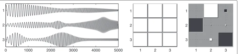
The above optimization problem can be tackled through various maximization algorithms. Our choice was to use a gradient ascent algorithm with momentum and adap-tive step sizes; after this gradient algorithm has run for 200 iterations, we use the BFGS algorithm implemented in MATLAB to improve the solution. The result of this optimization for the sources shown in Figure 1 is shown in Figure 2 forλ = 0.1, illustrating that IPA successfully recovers the original sources for this dataset.

3.3 Unicity of solution

In [14], we proved that a few mild assumptions on the sources, which are satisfied in the vast majority of real-world situations, suffice for a useful characterization of the global maxima of Problem (6): it turns out that there are infinitely many such maxima, and that they correspond either to correct solutions (i.e., the original sources up to permutation, scaling, and sign changes) or to singular matrices W. More specifically, we proved the following: assume that we have a set of complex-valued and linearly independent sources denoted bys(t), which have a PLF of 1 with one another. Consider also linear combinations

of the sources of the form y(t) = Cs(t) where C is a square matrix of appropriate dimensions. Further assume that the following conditions hold:

1. Neithersj(t)noryj(t)can identically be zero, for allj.

2. Cis non-singular.

3. The phase lag between any two sources is diﬀerent from 0 orπ.

4. The amplitudes of the sources,aj(t)= |sj(t)|, are

linearly independent.

Then, the only linear combination y(t) = Cs(t) of the sourcess(t)in which the PLF between any two compo-nents ofyis 1 isy(t) = s(t), up to permutation, scaling, and sign changes [14].

3.4 Comparison to ICA

The above result is simple, but some relevant remarks

should be made. If the optimum is found usingλ = 0

and the second assumption is not violated (or equiva-lently, det(C) = det(W)det(A) = 0, which is equivalent to det(W) = 0 if A is non-singular), then we can be certain that the correct solution has been found. How-ever, if the optimization is made using λ = 0, there is a possibility that the algorithm will estimate a bad solu-tion where, for example, some of the estimated sources are all equal to one another (in which case the PLFs between those estimated sources is trivially equal to 1). On the

other hand, if we use λ = 0 to guarantee that W is

non-singular, the unicity result stated above cannot be applied to the complete objective function. We call “non-singular solutions” and ““non-singular solutions” those in which det(W) = 0 and det(W) = 0, respectively. The result expressed in Section 3.3 is thus equivalent to stating that “all non-singular global optima of Equation (6) withλ=0 correspond to correct solutions”.

This contrasts strongly with ICA, where singular solu-tions are not an issue, because ICA algorithms attempt to ﬁnd independent sources and one signal is never inde-pendent from itself [7]. In other words, singular solutions always yield poor values of the objective function of ICA algorithms. Here we are attempting to estimate phase-locked sources, and any signal is perfectly phase-phase-locked with itself. Thus, one must always useλ=0 in the objec-tive function of Equation (6) when attempting to separate phase-locked sources.

We use a simple strategy to deal with this problem. We start by optimizing Equation (6) for a relatively large

value of λ(λ = 0.4), and once convergence has been

(6)

1 2 3 3

1 2 3

3

0 1000 2000 3000 4000 5000

3

Figure 2The three sources estimated by IPA (left), PLFs between them (middle), and the gain matrixWT_A_(right)._{Black squares represent} negative values of the gain matrix, while white squares represent positive values. Since the gain matrix is very close to a permutated diagonal matrix, we can conclude that IPA successfully recovered the sources, up to permutation, scaling, and sign change.

discussed above, whereas the final steps are done with a very low value ofλ, where the above unicity conditions are approximately valid. As the following experimental results show, this strategy can successfully prevent singular solu-tions from being found, while making the influence of the second term of Equation (6) on the final result negligible.

4 Experimental results

4.1 Data generation

As mentioned earlier, the main goal of this study is to study the applicability of IPA to real-world electrophysio-logical data from human brain EEG and MEG. The choice of the data for this study was not trivial, since we need to know the true sources in order to quantitatively mea-sure the quality of the results. On the one hand, to know the actual sources in the brain would require simultane-ous data from outside the scalp (EEG or MEG, which would be the mixed signals) and from inside the scalp (intra-craneal recordings, corresponding to the sources). If intra-craneal recordings are not available, results can-not quantitatively be assessed; they can only qualitatively be assessed by experts who can tell whether the extracted sources are meaningful or not. On the other hand, due to their extreme simplicity, synthetic data such as those used so far to illustrate IPA, shown in Figure 1, cannot be used to assess the usefulness of the method in real-world situations.

In an attempt to obtain “the best of both worlds”, we have generated a pseudo-real dataset from actual MEG recordings. By doing this, we know the true sources and the true mixing matrix, while still using sources that are of a nature similar to what one observes in real-world MEG. We begin by describing the process that we used to gen-erate a perfectly phase-locked dataset; we then explain how we modiﬁed these data to analyze non-perfect cases as well. It is important to stress that the generation pro-cess described below has no relation to the one used to generate the data of Figure 1, even though both processes generate sources with maximum PLF.

Our ﬁrst step was to obtain a realistic mixing matrix. To do so, we used the well-known EEGIFT software pack-age [29]. This packpack-age includes a real-world sample EEG dataset with 64 channels. Using all the default options of the software package, we extracted 20 independent com-ponents from the data of Subject 1 in that dataset. The results that was important for us, in this process, were not the independent components themselves (which were discarded), but rather the 64×20 mixing matrix. As dis-cussed in Section 3.1, we have opted for using a square mixing matrix, with little loss of generality. Therefore, we

selectedNrandom rows andN random columns of that

mixing matrix (without repetition), and formed anN×N mixing matrix from the corresponding values of the origi-nal 64×20 matrix. We will later show results for datasets ranging fromN = 2 toN = 5 sources; in the following, assume, for the sake of concreteness, thatN=4.

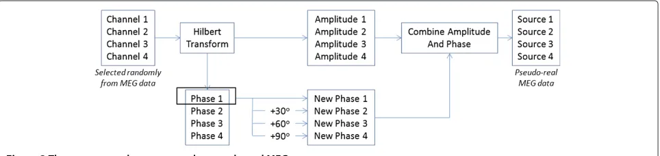
Having generated a physiologically plausible mixing matrix, the next step was to generate a set of four sources. For this, we used the MEG dataset studied previously in [30]h, which has 122 channels with 17,730 samples per channel. The sampling frequency is 297 Hz, and the data have already been subjected to low-pass filtering with cut-off at 90 Hz. Since band-pass filtering is a very common preprocessing step in the analysis of MEG data [20-22] and is useful for the use of the Hilbert transform, we performed a further band-pass filtering with no phase distortion, keeping only the 18–24 Hz bandi. The result-ing filtered data were used to generate a complex signal through the Hilbert transform; these data were whitened as described in Section 3.1, and from the whitened data we extracted the time-dependent amplitudes and phases.

(7)

channel with a constant phase lag ofπ₆radians. The phase of the third channel was replaced with the phase of the first channel with a constant phase lag of π₃ radians, and that of the fourth channel with the phase of the first chan-nel with a lag of π₂ radians. The amplitudes of the four sources were kept as the original amplitudes of the four random channels themselves. The process is illustrated in Figure 3. The above process, including the choice of the 4×4 submatrix, was repeated 100 times, with different ini-tializations of the random number generator. This way of constructing the data ensured that the sources were fully phase-locked.

We also constructed datasets in which the sources were not perfectly phase locked. For this, we used the same 100 sets of sources, but with those sources now corrupted by phase jitter: each sampletof each sourcejwas multiplied byeiδj(t)_{, where the phase jitter}_δ

j(t)was drawn from a

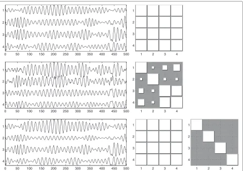
ran-dom Gaussian distribution with zero mean and standard deviationσ. We tested IPA forσfrom 0 to 20 degrees, in 5 degrees steps. One example withσ=5 degrees is shown

in Figure 4, and one with σ = 20 degrees is shown in

Figure 5.

Finally, we studied the eﬀect of N on the results of the proposed algorithm. We created 100 datasets simi-lar to the jitterless datasets mentioned earlier, usingN = 2, 3 and 5. In all of these, and similarly to the data with N=4, we used sources with phase lags multiple ofπ₆.

4.2 Results

We measured the separation quality using two measures: the Amari performance index (API) [31] and the well-known signal-to-noise ratio (SNR). The API measures how far the gain matrixWTAis from a permutated diag-onal matrix; the SNR measures how far the estimated sources are from the true sources. In summary, the API measures the quality of the estimation of the mixing matrix, while the SNR measures the quality of the estima-tion of the sources themselves.

Figure 6 presents the means and standard deviations of these measures for the 100 runs mentioned in Section 4.1, for each of the jitter levels. The results indicate that IPA

has very good performance on the jitterless case, in data of this kind, and that this level of performance is approx-imately maintained even in the presence of low levels of phase jitter, up to 5 degrees of standard deviation. Some deterioration in performance occurs from 5 to 10 degrees of phase jitter standard deviation, but with a SNR of 27 dB and an API below 0.1 the sources can still be considered to be well estimated.

The results for high jitter levels (sigmaequal to 15 or 20 degrees) show that there is a limit to IPA’s robust-ness; this limit lies somewhere between 10 and 15 degrees. Equivalently, in terms of the PLF, the algorithm shows good robustness to PLF values smaller than 1 as long as they are above 0.95, but below that value its performance deteriorates progressively up to a PLF of approximately 0.9, at which point only partial separations are obtained.

Figure 7 shows the eﬀect of varying the number of

sources N. The ﬁgure shows that IPA can handle

val-ues of N up to N = 5 with only a slight decrease in

performance.

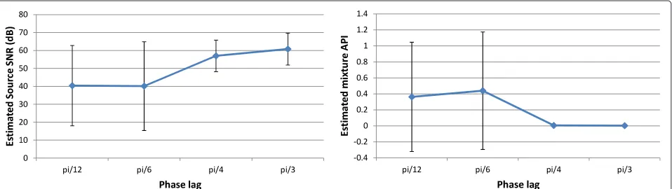
Figure 7 also shows something rather peculiar: forN= 2, the results are mediocre (with an average API around 0.4)j. This is not an eﬀect of lowering the number of sourcesN, but rather an indirect eﬀect of the phase lag between the sources. To verify this, we generated datasets of jitterless data withN = 2, using phase lags of ₁₂π, 2₁₂π (the value used in Figure 7), 3₁₂π, and 4₁₂π (100 datasets for each of these values). Figure 8 shows that a phase lag of2₁₂π yields poor API values, as we already knew, but 3₁₂π yields very good values. Naively, one could conclude that when the sources have a phase lag of 2₁₂π, or less, the separation cannot be accurately performed.

The effect is, however, not so clear-cut. The results for N = 3, 4, 5 also involve sources with phase lags of π₆, but the API values for those experiments are very good. We do not have a solid explanation for this fact; we conjec-ture that the presence of some pairs of sources with larger phase lags (e.g., for N = 4, the first and third sources have a phase lag of π₃ and the first and fourth sources have a phase lag of π₂) aids in the separation of all the sources.

(8)

1 2 3 4 3

4

0 50 100 150 200 250 300 350 400 450 500 4

3 2 1

1 2 3 4

1

2

3

4

0 50 100 150 200 250 300 350 400 450 500 4

3 2 1

1 2 3 4

1

2

3

4

1 2 3 4

1

2

3

4 0 50 100 150 200 250 300 350 400 450 500

4 3

Figure 4Example of a dataset whereσ=5degrees.Only a short segment of the signals is shown, for clarity. Top row: original sources (left) and PLFs between them (right). Middle row: mixed signals (left) and PLFs between them (right). Bottom row: estimated sources, after manual

compensation of permutation, scaling, and sign (left); PLFs between them (middle); and the gain matrixWT_A_{(right). The gain matrix is virtually} equal to the identity matrix, indicating a correct separation.

5 Discussion

IPA has a parameter,λ, which controls the relative weights given to the optimization of the PLF matrix and to the penalization of close-to-singular solutions. Our optimiza-tion procedure starts with a high value of λ, which is lowered as the optimization progresses. We confirmed that this variation of the parameter’s value is necessary: the quality of the results is noticeably degraded ifλis kept at a constant value, no matter how high or low it is. Table 1 confirms this: whileλ = 0.1, the best fixed value, yields decent results, the results with a varying value of λare considerably better. Furthermore, although the final epoch in the optimization is not done withλ=0, we have veri-fied that the results are virtually the same as if we had used

λ=0 at the last epoch.

The above paragraph illustrates something already men-tioned in Section 3.4: separation of phase-locked sources is a non-trivial change from ICA because there are wrong, singular solutions that yield exactly the same values of the PLF matrix as the correct non-singular solutions. Our

approach to distinguish these two types of solutions con-sists in adding a term depending on the determinant of the matrixW. This approach works correctly, as our results show. However, it is perhaps inelegant to do this through matrix W, instead of doing it directly through the esti-mated sources. It would be preferable to replace this term with one depending directly on the estimated sources.

The size of the optimization variable,W, isN2; there areNconstraints on this variable, yieldingN(N−1) inde-pendent parameters. This means that the IPA algorithm is quadratic in the number of sourcesN, which is the main reason why we do not present results forN > 5; while running IPA on 100 datasets withN=2 takes a few hours, doing so forN=5 takes several days.

(9)

1 2 3 4 1

2

3

4

0 50 100 150 200 250 300 350 400 450 500 4

3 2 1

1 2 3 4

1

2

3

4

0 50 100 150 200 250 300 350 400 450 500 4

3 2 1

1 2 3 4

1

2

3

4

1 2 3 4

1

2

3

4 0 50 100 150 200 250 300 350 400 450 500

4 3 2 1

Figure 5Example of a dataset whereσ=20degrees.Only a short segment of the signals is shown, for clarity. Top row: original sources (left) and PLFs between them (right). Middle row: mixed signals (left) and PLFs between them (right). Bottom row: estimated sources, after manual compensation of permutation, scaling, and sign (left); PLFs between them (middle); and the gain matrixWT_A_{(right). The gain matrix has signiﬁcant} values outside the diagonal, indicating that a complete separation was not achieved. Nevertheless, the largest values are in the diagonal, corresponding to a partial separation.

results indicate that IPA has some robustness to PLFs smaller than 1, but the sources still need to exhibit con-siderable phase locking for the separation to be accurate; weaker synchrony results only in partial separation. Note, however, that the partially separated data are usually still closer to the true sources than the original mixtures.

The comments made in the previous paragraph raise an additional optimization challenge: if the true sources have PLFs smaller than 1, optimization of the objec-tive function in Equation (6) can lead to overﬁtting. The results presented here show that IPA has some robust-ness to sources which have a PLF smaller than 1, while

(10)

Figure 7Eﬀect of applying IPA to pseudo-real MEG data with varying values ofN: SNR (left) and API (right).

being stationary (since the phase jitter is stationary, the distribution of the PLF does not vary with time). In real-world cases, it is likely that the PLF is non-stationary: for example, some sources may be phase-locked at the start of the observation period and not phase-locked at its end. While simple techniques such as windowing can be devised to tackle smaller time intervals where stationarity is (almost) verified, one would still need to find a way to integrate the information from different intervals. Such integration is out of the scope of this article.

One interesting extension of this article would be the separation of speciﬁc types of systems, such as van der Pol oscillators [27]. For those, fully entrained oscillators may even present a PLF< 1, and a diﬀerent measure of syn-chrony, tailored to those oscillators, may need to be used. Such a study would fall out of the scope of this article. Nevertheless, it is expected that additional knowledge of the oscillator type can be exploited to improve the algo-rithm’s performance or its robustness to deviations from the ideal case.

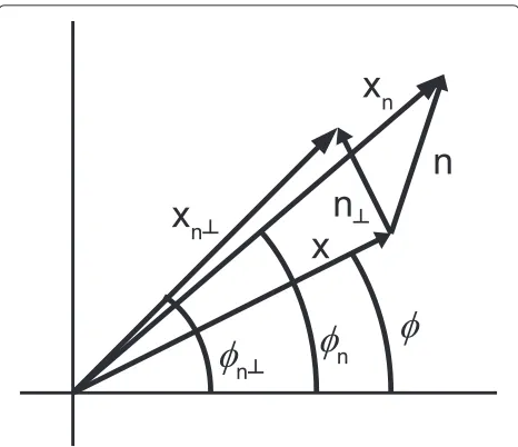
One can derive a relationship between additive Gaussian noise (e.g., from the sensors) and the phase jit-ter used throughout this article. Figure 5 depicts, in the complex plane, a sample of a noiseless signal x(t) ≡

a(t)eiφ(t)_{, to which complex noise}_n₍_t_{) is added to form} the noisy signal xn ≡ a(t)eiφ(t) + n(t)k. That ﬁgure

also shows n⊥(t), which is the projection of n(t) on the direction orthogonal to x(t), and xn⊥(t) ≡ x(t) +

n⊥(t). Also depicted are φ (t), φ_n(t) and φ_n_⊥(t), which are deﬁned as the phases of x(t), xn(t) and xn⊥(t),

respectively.

It can easily be shown that, if|n(t)| << |x(t)| = a(t), then φn(t) ≈ φn⊥(t) ≈ φ (t) + n_a⊥₍(_tt₎) [32]. This is an important relationship, because it shows that, under addi-tive noise, portions of the signal with a large amplitude will have a better phase estimate than portions with a small amplitude, in which even small amounts of additive noise can severely disrupt the phase estimation. We thus believe that the PLF quantity, while attractive and elegant in theory, and despite working well with low amounts of additive noise [14], will probably need to be changed to factor in the amplitude in an appropriate way to deal with applications where considerable amounts of additive noise are present.

6 Conclusion

We have shown that IPA can successfully separate phase-locked sources from linear mixtures in pseudo-real MEG data. We showed that IPA tolerates deviations from the

(11)

Table 1 Values of SNR and API for jitterless data withN=3, for various ﬁxed values ofλ, as well as for the varying-lambda strategy detailed in the text

λ 0.025 0.05 0.1 0.2 0.4

SNR Fixed 17.5±21.2 27.5±18.0 34.4±4.3 27.2±3.6 13.5±5.5

Varying 48.9±8.7

API Fixed 0.795±0.570 0.369±0465 0.048±0.057 0.079±0.027 0.327±0.097

Varying 0.013±0.015

While the best ﬁxed value,λ=0.1, yields decent results, the results using a varying value ofλare consistently better, with a large margin.

ideal case, yielding excellent results for low amounts of phase jitter, and that it exhibits some robustness to mod-erate amounts of phase jitter. We also showed that it can

handle numbers of sources up to N = 5. We believe

that these results bring us closer to the goal of suc-cessfully separating phase-locked sources in real-world signals.

Endnotes

a_{In EEG and MEG, the sources are not individual}

neu-rons, whose oscillations are too weak to be detected from outside the scalp. In these cases, the sources are populations of closely located neurons oscillating together.

b_{The term “real-valued” is used here to distinguish from} other phase-based algorithms where a complex quantity is used [14].

c_{Technically, this condition could be violated in a set with} zero measure. Since we will deal with a discrete and ﬁnite number of time points, no such sets exist and this techni-cality is not important.

d_{We will also show results where this phase diﬀerence is} not exactly constant; see Figure 6.

Figure 9Diagram illustrating the relationship between phase jitter and additive noise.A single time sample is shown, and the time argument has been dropped for simplicity.

e_{These assumptions are not as restrictive as they may} sound; see Section 3.1.

f_{This is usually called the over-determined case. The}

under-determined case, where A has fewer rows than

columns, is more diﬃcult and is not addressed here. g_{There are more rigorous criteria that can be used to}

choose N. Two very popular methods are the Akaike

information criterion and the minimum description length. It is out of the scope of this article to discuss these two criteria; the reader is referred to [7] and references therein for more information.

h_Freely _available _from _{http://research.ics.tkk.ﬁ/ica/} eegmeg/MEG data.html.

i_{The choice of this speciﬁc band is rather arbitrary. The} band is narrow enough that the Hilbert transform will allow correct estimation of instantaneous amplitude and phase, but wide enough that the instantaneous frequency of the signals retains some variability. The passband is also of a similar width as in typical studies using MEG [20]. j_{It might appear contradictory that the average SNR has a} good value, 40 dB, when the average API has a mediocre score. In reality, when the standard deviation of the SNR is very high, it is usually an indication that the separation is poor. As an example, consider a case where one source is very well estimated, with an SNR of 80 dB, and one is poorly estimated, with an SNR of 0 dB. The average SNR would be 40, but with a very high standard-deviation. Good values of the average SNR are indicators of a good separation only when the standard-deviation of the SNR is small.

k_{In most real applications, one will be dealing with} mod-els consisting of real signals to which real-valued noise is added. However, the linearity of the Hilbert transform allows the same type of analysis for that case as for the case of complex signals with complex additive noise which is considered here.

Competing interests

The author declare that they have no competing interests.

Acknowledgements

This work was partially supported by project DECA-Bio of Instituto de Telecomunicacoes, PEst-OE/EEI/LA0008/2011.

Author details

(12)

University Press), Cambridge, MA, 2001)

2. JM Palva, S Palva, K Kaila, Phase synchrony among neuronal oscillations in the human cortex. J. Neurosci.25(15), 3962–3972 (2005)

3. JM Schoﬀelen, R Oostenveld, P Fries, Imaging the human motor system’s beta-band synchronization during isometric contraction. NeuroImage.

41, 437–447 (2008)

4. PJ Uhlhaas, W Singer, Neural synchrony in brain disorders: relevance for cognitive dysfunctions and pathophysiology. Neuron.52, 155–168 (2006) 5. PL Nunez, R Srinivasan, AF Westdorp, RS Wijesinghe, DM Tucker, RB

Silberstein, PJ Cadusch, EEG coherency I: statistics, reference electrode, volume conduction, Laplacians, cortical imaging, and interpretation at multiple scales. Electroencephalogr. Clin. Neurophysiol.

103, 499–515 (1997)

6. R Vigário, J Särelä, V Jousmäki, M Hämäläinen, E Oja, Independent component approach to the analysis of EEG and MEG recordings. IEEE Trans. Biomed. Eng.47(5), 589–593 (2000)

7. A Hyv¨arinen, J Karhunen, E Oja,Independent Component Analysis. (Wiley, New York, 2001)

8. M Akhtar, W Mitsuhashi, C James, Employing spatially constrained ICA and wavelet denoising for automatic removal of artifacts from multichannel EEG data. Signal Process.92, 401–416 (2012) 9. M de Vos, L de Lathauwer, S van Huﬀel, Spatially constrained ICA

algorithm with an application in EEG processing. Signal Process.

91, 1963–1972 (2011)

10. D Lee, H Seung, Algorithms for non-negative matrix factorization. Adv. Neural Inf. Process. Syst.13, 556–562 (2001)

11. TH Chan, WK Ma, CY Chi, Y Wang, A convex analysis framework for blind separation of non-negative sources. IEEE Trans. Signal Process.

56, 5120–5134 (2008)

12. R de Frein, S Rickard, The synchronized short-time-Fourier-transform: properties and deﬁnitions for multichannel source separation. IEEE Trans. Signal Process.59, 91–103 (2011)

13. S Hosseini, Y Deville, H Saylani, Blind separation of linear instantaneous mixtures of non-stationary signals in the frequency domain. Signal Process.89, 819–830 (2009)

14. M Almeida, JH Schleimer, J Bioucas-Dias, R Vig´ario, Source separation and clustering of phase-locked subspaces. IEEE Trans. Neural Netw.

22(9), 1419–1434 (2011)

15. M Almeida, J Bioucas-Dias, R Vig´ario, inProceedings of the International Conference on Independent Component Analysis and Signal Separation, vol. 6365. Independent phase analysis: separating phase-locked subspaces, (2010), pp. 189–196

16. A Ziehe, KR M üller, inInternational Conference on Artificial Neural Networks. TDSEP—an efficient algorithm for blind separation using time structure, (1998), pp. 675–680

17. C Torrence, GP Compo, A practical guide to wavelet analysis. Bull. Am. Meteorol. Soc.79, 61–78 (1998)

18. AV Oppenheim, RW Schafer, JR Buck,Discrete-Time Signal Processing. (Prentice-Hall International Editions, Englewood Cliﬀs, NJ, 1999) 19. MLV Quyen, J Foucher, JP Lachaux, E Rodriguez, A Lutz, J Martinerie,

FJ Varela, Comparison of Hilbert transform and wavelet methods for the analysis of neuronal synchrony. J. Neurosci. Methods.111, 83–98 (2001) 20. F Varela, JP Lachaux, E Rodriguez, J Martinerie, The Brainweb: phase

synchronization and large-scale integration. Nat. Rev. Neurosci.

2, 229–239 (2001)

21. E Niedermeyer, FHL da Silva,Electroencephalography: Basic Principles, Clinical Applications, and Related Fields. (Lippincott Williams and Wilkins, Philadelphia, 2005)

22. P Nunez, R Srinivasan,Electric Fields of the Brain: the Neurophysics of EEG. (Oxford University Press, New York, 2006)

23. B Gold, AV Oppenheim, CM Rader, inSymposium on Computer Processing in Communications. Theory and implementation of the discrete Hilbert transform, (1973)

27. E Izhikevich,Dynamic Systems in Neuroscience. (MIT Press, Cambridge, MA, 2007)

28. M Almeida, R Vig´ario, J Bioucas-Dias, inProceedings of the International Conference on Latent Variable Analysis and Signal Separation, vol. 7191. The role of whitening for separation of synchronous sources, (2012), pp. 139–146

29. T Eichele, S Rachakonda, B Brakedal, R Eikeland, VD Calhoun, EEGIFT: group independent component analysis for event-related EEG data. Comput. Intell. Neurosci.2011, 1–9 (2011)

30. R Vigário, V Jousmäki, M Hämäläinen, R Hari, E Oja, inAdvances in NIPS. Independent component analysis for identification of artifacts in magnetoencephalographic recordings, (1997)

31. S Amari, A Cichocki, HH Yang, inAdvances in NIPS, vol. 8. A new learning algorithm for blind signal separation, (1996), pp. 757–763

32. A Carlson, P Crilly, J Rutledge. Communication Systems: An Introduction to Signals and Noise in Electrical Communication (McGraw-Hill, New York, 2001)

doi:10.1186/1687-6180-2013-32

Cite this article as:Almeidaet al.:Separation of phase-locked sources in pseudo-real MEG data.EURASIP Journal on Advances in Signal Processing2013 2013:32.

Submit your manuscript to a

journal and beneﬁ t from:

7Convenient online submission

7Rigorous peer review

7Immediate publication on acceptance

7Open access: articles freely available online

7High visibility within the ﬁ eld

7Retaining the copyright to your article