Topological Active Volumes
N. Barreira
Grupo de Visi´on Artificial y Reconocimiento de Patrones (VARPA), LFCIA, Departamento de Computaci´on, Universidade da Coru˜na, 15071 A Coru˜na, Spain
Email:[email protected]
M. G. Penedo
Grupo de Visi´on Artificial y Reconocimiento de Patrones (VARPA), LFCIA, Departamento de Computaci´on, Universidade da Coru˜na, 15071 A Coru˜na, Spain
Email:[email protected]
Received 29 December 2003; Revised 4 February 2005
The topological active volumes (TAVs) model is a general model for 3D image segmentation. It is based on deformable models and integrates features of region-based and boundary-based segmentation techniques. Besides segmentation, it can also be used for surface reconstruction and topological analysis of the inside of detected objects. The TAV structure is flexible and allows topological changes in order to improve the adjustment to object’s local characteristics, find several objects in the scene, and identify and delimit holes in detected structures. This paper describes the main features of the TAV model and shows its ability to segment volumes in an automated manner.
Keywords and phrases:image segmentation, 3D reconstruction, active nets, active volumes.
1. INTRODUCTION
The scene in a 3D image is usually made of an object or sev-eral objects. The segmentation task consists of isolating the points that belong to each object from the image and inte-grating them into a coherent and consistent model of the de-tected structures. Unfortunately, the detection of objects in-side 3D data is difficult due to the complex topology of the objects and the cost of the operations in a 3D space. Further-more, the available means of acquisition introduce noise in data, so direct segmentation is often inadequate and the use of an advanced segmentation technique is needed.
There are many approaches for segmentation proposed in the literature. Nowadays, level set methods and de-formable models have become two of the most promising techniques for segmentation, mapping, tracking, and mod-elling tasks. Level set methods were introduced by Osher and Sethian [1] and have found several applications in image pro-cessing, such as segmentation and reconstruction of complex shapes [2,3] due to their ability to perform topological trans-formations. However, level sets’ formulation is more com-plex than deformable models’. Deformable models were in-troduced by Kass et al. [4] in 2D as explicit deformable con-tours and generalised to the 3D case by Terzopoulos et al. [5]. In recent years, many models have been developed for the treatment of 3D scenes [6,7,8]. They have tried to solve some of the limitations of classical deformable models, such
as the sensitivity to the initialisation or the parametric def-inition of the model, which restricts their topology to seg-ment simple objects. These models have also adapted their operation to concrete domains by means of the definition of different energy terms or the use of several topologies. In par-ticular, some models have increased their degree of flexibility, providing a way to perform topological transformations on their structures [9,10]. However, all these models are mainly interested in surface extraction and shape recovery, not in the treatment of the whole detected solid.
In this paper a general 3D deformable model is proposed, thetopological active volumes, as an extension of the topolog-ical active nets[11], focused on segmentation tasks by means of a volumetric distribution of nodes. It is fully automatic, so no a priori knowledge is needed to initialise the model. It also integrates information of edges and regions in the adjustment process and allows to obtain topological infor-mation inside the objects found. The model has a dynamic behaviour by means of topological changes in its structure which enables accurate adjustments and the detection of sev-eral objects in the scene.
2. TOPOLOGICAL ACTIVE VOLUMES
The model presented in this paper is an extension of topolog-ical active nets [11] to the 3D world. Its operation is focused on extraction, modelization, and reconstruction of volumet-ric objects present in the scene.
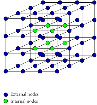
A topological active volume (TAV) is a 3D structure com-posed by interrelated nodes, where the basic repeated struc-ture is a cube (Figure 1). Parametrically, a TAV is defined as v(r,s,t) = (x(r,s,t),y(r,s,t),z(r,s,t)), where (r,s,t) ∈ ([0, 1]×[0, 1]×[0, 1]). The state of the model is governed by an energy function defined as follows:
E(v)=
1
0
1
0
1
0 Eint
v(r,s,t)
+Eext
v(r,s,t)dr ds dt,
(1)
where Eint and Eext are the internal and the external
en-ergy of the TAV, respectively. The former controls the shape and the structure of the net. Its calculus depends on first-and second-order derivatives which control contraction first-and bending, respectively. The internal energy term is defined by
Eint
v(r,s,t)
=αvr(r,s,t)2+vs(r,s,t)2+vt(r,s,t)2
+βvrr(r,s,t)2+vss(r,s,t)2+vtt(r,s,t)2
+ 2γvrs(r,s,t)2+vrt(r,s,t)2+vst(r,s,t)2, (2)
where subscripts represent partial derivatives andα,β, and γare coefficients that control the smoothness of the net. In order to compute the energy, the parameter domain [0, 1]× [0, 1]×[0, 1] is discretized as a regular grid defined by the in-ternode spacing (k,l,m) and the first and second derivatives are estimated using the finite differences technique in 3D.
Eextrepresents the characteristics of the scene that guide
the adjustment process. As can be seen inFigure 1, the model has two types of nodes: internal and external. Each type of node is used to represent different features of the object: the external nodes fit the surface of the object and the internal nodes model the internal topology of the object. So the ex-ternal energy has to be different for both types of nodes. This fact allows the integration of information based on disconti-nuities and information based on regions. The former is as-sociated to external nodes and the latter, to internal nodes. In this model, the external energy term is defined as
Eext
v(r,s,t)
=ω fIv(r,s,t)
+ ρ
ℵ(r,s,t)
p∈ℵ(r,s,t)
1
v(r,s,t)−v(p)fIv(p), (3)
External nodes Internal nodes
Figure1: A TAV grid.
whereωandρare weights,I(v(r,s,t)) is the intensity value of the original image in the positionv(r,s,t),ℵ(r,s,t) is the neighbourhood of the node (r,s,t), and f is a function asso-ciated to the image intensity and defined differently for both types of nodes.
On one hand, if the objects to detect are dark and the background is bright, the energy of an internal node will be minimum when it is on a point with a low grey level. On the other hand, the energy of an external node will be minimum when it is on a discontinuity and on a light point outside the object. In this situation, function f is defined as
fI(v)=
hI(v)n
for internal nodes,
hImax−I(v)n +ξGmax−G(v)
for external nodes, (4)
whereξis a weighting term,ImaxandGmaxare the maximum
intensity values of imageIand the gradient imageG, respec-tively, I(v) andG(v) are the intensity values of the original image and the gradient image in node positionv(r,s,t),I(v)n is the mean intensity in ann×n×ncube, andhis an appro-priate scaling function.
Otherwise, if the objects are bright and the background is dark, the energy of an internal node will be minimum when it is on a point with a high grey level and the energy of an external node will be minimum when it is on a discontinuity and on a dark point outside the object. In such a case, func-tion f is defined as
fI(v)=
hImax−I(v)n
for internal nodes,
hI(v)n
+ξGmax−G(v)
for external nodes, (5)
TAV initialisation
Energy min.
TAV readjustment
Energy min.
External nodes badly
located ? Yes
Connection breaking Energy
min.
Energy min.
Hole creation
Internal nodes badly
located ? Yes
Hole nodes badly
located ? Yes
No
No
No End Connection
breaking Energy
min.
Figure2: Stages in the TAV adjustment process.
3. METHODOLOGY
The adjustment process of the TAV has several stages, as shown inFigure 2.
The first stage consists of placing the 3D structure in the image. The nodes cover the whole image and they are lo-cated in such a way that the internodal distance is the same in each dimension. This way, the model is able to detect an object in the image even if it were placed at different posi-tions.
The energy minimisation is performed locally using a greedy algorithm. With this algorithm, the energy value for each node is computed in several positions of the 3D image (the current position and its 26 neighbour positions) at every step of the minimisation process and the best one is chosen as the next position of the node. The process finishes when the TAV reaches a stable situation, that is, when the energy of each node in the TAV is minimal.
Once the mesh reaches a stable situation, the number of nodes is recomputed in order to adjust the size of the TAV to the size of the object, that is, if the object is wider than high, the number of nodes in the x-axis will be larger than the number of nodes in the y-axis. After that, the mesh, which covered the whole image in the beginning, is centred around the object. The readjustment of the mesh allows the acquisi-tion of the same distribuacquisi-tion of nodes independently of the position of the object in the image [12]. Then the minimisa-tion process is repeated.
Figure3: Differences between an adjusted TAV without and with topological changes.
The physical characteristics of the mesh do not enable the perfect adaptation of the nodes to the objects, so some kind of topological transformation on the TAVs are neces-sary to achieve a good adjustment. This way, the restric-tions of a fixed topology can be avoided. The first topolog-ical change consists of the rupture of connections between external nodes which are wrongly placed in the image. This allows a perfect adjustment to the surfaces of the objects, the detection of several objects in the image, and the generation of external holes in the mesh. The second topological change is the creation of holes in the inside of the mesh in order to delimit the holes of the objects. The analysis of the internal nodes and the rupture of connections allow the second type of topological changes.
3.1. Rupture of connections
The TAVs have the ability to perform topological changes that give more flexibility to their structure and avoid the limitations of a fixed topology as we can see in Figure 3. The changes consist of removing connections between nodes. They allow to (a) increase the fitting accuracy on those zones where a greater definition is required, (b) detect two or more objects in the image through the generation of 2 or more sub-TAVs, and (c) model the found objects and adjust to external holes.
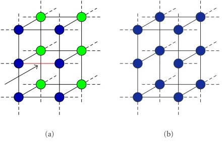
The process of breaking a connection takes place only be-tween external nodes that are badly located after the min-imisation process. This removal will affect the elementary structures, that is, the cubes the nodes belong to. Once the connection between two external nodes has disappeared, the nodes have a greater freedom of movement. Besides, the rup-ture of a link implies that some internal nodes will become external asFigure 4shows. The new external nodes will al-low a greater definition and adjustment in the area where the breaking takes place.
The breaking process has one restriction: the cubic struc-ture of the model must be maintained (all the nodes and connections must belong to, at least, one cube) because TAV model performs, not only surface extraction, but also volume segmentation and so, isolated nodes, connections, or planes do not provide useful information. This is why connections will not be erased if the cubic structure is broken.
(a) (b)
Figure4: Conversion of internal nodes to external nodes. (a) Be-fore the rupture of the marked connection. (b) After the rupture of the connection. Light nodes represent internal nodes and dark ones external nodes.
b
a
(a)
a b
c d
(b)
Figure5: Multiple breakings. The marked connections must be si-multaneously broken because (a) the rupture of connectiona re-sults in connectionbnot belonging to any cube; (b) if one labelled connection is broken, the rest of the connections will not belong to any cube.
that share the connection are checked in order to find a com-bination of connection breakings that maintain the cubic structure. Nevertheless, a connection will only be broken if its side nodes are badly placed.Figure 5depicts two cases of this particular situation. InFigure 5a, if connectionais bro-ken, connection bwill not belong to any cube as there are no cubes over it. Connectionamust be broken together with connectionb. Notice that connectionbcan be broken with-out connection a because connection a is part of another cube.Figure 5bshows an example where the connectionsa, b,c, anddmust be broken simultaneously in order to main-tain the cubic structure.
After the minimisation process, the external nodes badly located are chosen by their gradient distance. Gradient dis-tance is computed through an extension of midpoint algo-rithm [13] in 3D. A node will be badly located if its gradient distance is greater than a certain threshold, which is com-puted by Tchebycheff’s theorem [14]. This theorem
iden-tifies the outliers within a population. Thus, an external nodevext(r,s,t) will be badly located if its gradient distance,
GDvext(r,s,t), verifies that
GDvext(r,s,t)> µGDvext+cσGDvext, (6)
where µGDvext and σGDvext represent the average and the
standard deviation of the gradient distance of the external nodes, respectively.cis a constant so that 1/c2is the
percent-age of correctly placed nodes. We have used a value ofc=2. The gradient distance is computed as follows:
GDvext(r,s,t)=min GD
k
vext(r,s,t) ∀k∈κ, (7)
where κ is the set of possible directions defined by a 26-neighbourhood.
Once the external nodes badly placed are delimited, the connection to break is selected. It is the connection between the worst placed node and its worst neighbour. After break-ing a connection and performbreak-ing the topological changes, the TAV is minimised again. This process is repeated until there is no node which fulfils (6).
In order to guide the breaking process and avoid anar-chical breakings, a cut priority is used. The cut priority of each node is initially 1 and is doubled every time a breaking takes place in the cube the node belongs to. The gradient dis-tance is multiplied by the cut priority and the result is used instead of the gradient distance value in (6). This way, the gradient distance is weighted, which increases the probabil-ity that new breakings will be performed in the direction of previous breakings.
Figures6aand6bshow the next breaking after the rup-ture of a connection in the upper cube. In these figures, the external nodes are labelled with the gradient distance and the gradient distance weighted by the cut priority, respectively. Without cut priority, the node with greater gradient distance and its worst placed neighbour share the connection to break, asFigure 6ashows. However, if cut priority is considered, af-ter the first breaking, the nodes in the upper cube double its initial priority to 2 which weights the gradient distance, as Figure 6bshows. In this case, the next connection to break is in the cube where the first breaking has taken place.
Figures6cand6ddepict the consequences of anarchical and organised breakings, that is, without or with cut prior-ity. If the cut priority is not considered, the breakings will be chaotic and there could be groups of linked cubes badly placed whose connections cannot be broken (threads). When the cut priority is used, the probability of thread formation diminishes.
5 0
7 10 4 6
5
9 8
12
9 7
(a)
2∗5 2∗0
2∗7 2∗10 2∗4 2∗9 2∗6 2∗8
1∗5 1∗12
1∗9 1∗7
(b)
(c) (d)
Figure6: Next connection to break (a) without cut priority and (b) with cut priority (the first value is the cut priority and the second one the gradient distance). (c) Breaks without cut priority and (d) with cut priority.
3.2. Hole creation
The topological information provided by the distribution of the internal nodes allows us to know the inner morphology of detected objects. This information can be used to detect inner holes in the objects.
If there is a hole in an object, the internal nodes will try to avoid it and there will be tension between them, so the value of the internal energy will be high (see (2)). The inter-nal nodes will also have a high value of exterinter-nal energy due to the characteristics of the hole. For example, if the object is dark and the background is light, the holes in the object will be light, too. In this case, the energy value of an internal node is minimum when the node is in a dark voxel (see (4)). But the holes are light and then, if an internal node is inside a hole, its energy value will not be minimum.
Tchebycheff’s theorem [14] is also employed to find the internal nodes inside a hole. An internal node is supposed to be inside a hole if its energy value,Evint(r,s,t), verifies that
Evint(r,s,t)> µEvint+ 3σEvint, (8)
where µEvint andσEvint(r,s,t) represent the average and the
standard deviation of the total energy, that is, the sum of the internal and external energies of the internal nodes.
(a) (b)
Figure7: Topological adaptive changes in TAVs. (a) The mesh is divided. (b) A hole in the mesh is generated.
Once the set of internal nodes inside the hole is known, the hole is created from a cube of internal nodes: one of them is the worst placed and the other ones are also badly placed nodes.
The hole must be composed of external nodes as they must be anchored to the surface of the hole. However, the aim of the external nodes is contracting around the object whereas the nodes inside a hole have to expand themselves towards the surfaces of the hole. So, there will be three kinds of nodes:internal nodes,external nodes outside the hole, and external nodes inside the hole. Each kind of node has its own external energy function, which replaces the function defined in (4). The new energy function is defined as
fI(v)=
hI(v)n
for internal nodes,
hImax−I(v)n +ξGmax−G(v)
for external nodes,
hImax−I(v)n +GDmin(v)
for hole nodes, (9)
where GDmin(v) represents the minimum gradient distance
(a)
(b)
(c)
(d)
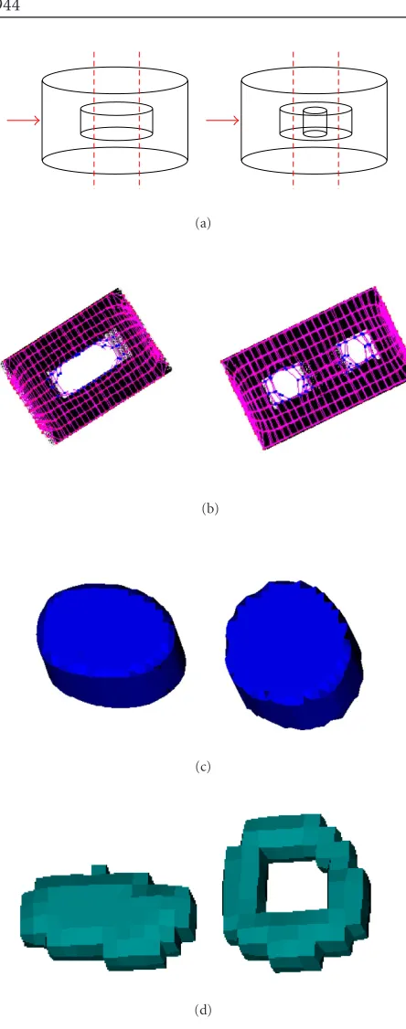
Figure 8: Images with inner holes. (a) Diagrams of the objects. (b) Cross-section of the objects defined by the arrows and the dot-ted lines ofFigure 8a. (c) 3D reconstruction of external surfaces. (d) 3D reconstruction of hole surfaces.
Once the holes are created in the mesh, a process of rup-ture of connections and energy minimisations is performed as it has been explained inSection 3.1but, in this case, the breakings would take place between external nodes inside the hole.
Figure9: Results obtained on artificial noisy images. The first row shows the original image, the second row shows the segmented meshes, and the last row shows the 3D reconstruction of the de-tected object from the external nodes.
Figure 8shows some examples of images with inner holes and the results of segmentation process. These 3D images are cylinders with an inner hole as shown in the 3D diagram inFigure 8a.Figure 8bshows a cross-section of the 3D im-age defined by the dotted lines in the imim-age of Figure 8a. The point of view of these sections is shown by the arrow in Figure 8a. In these images, the internal adaptation of the TAV to the surface of the holes can be seen. Figures8aand8bshow the 3D reconstruction of the external surface and the hole, respectively. In order to show the adjustment of the mesh, the reconstruction is based on the coordinates of the exter-nal nodes and no smooth technique was used to enhance the results.
4. RESULTS
Table1: Number of nodes and parameters of TAVs used inFigure 9.
Image TAV size Param.Eint Param.Eext
(x,y,z) (α,β,γ) (ω,ρ,ξ)
Left 11, 9, 6 3.1, 10−5, 10−5 2.0, 5.0, 3.5
Right 15, 15, 3 4.0, 10−5, 10−5 5.0, 5.0, 3.0
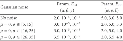
Table2: Parameters used in the segmentation processes of the noisy images. The first row shows the parameters typically used to process images without noise.
Gaussian noise Param.Eint Param.Eext
(α,β,γ) (ω,ρ,ξ)
No noise 2.0, 10−5, 10−5 5.0, 3.0, 5.0 µ=0,σ∈[5, 15] 3.0, 10−5, 10−5 2.0, 5.0, 3.3 µ=0,σ∈[16, 25] 3.0, 10−5, 10−5 2.0, 5.0, 4.0 µ=0,σ∈[26, 35] 3.5, 10−5, 10−5 2.0, 5.5, 4.0
Figure 9shows some examples of segmentation on arti-ficial images with 255 grey levels. The objects are dark and the background, light. The first image had 80slicesand the second, 40. The size of each slice was 256×256. The initial TAV had 8×8×8 nodes in all the examples. Each slice of these 3D images has Gaussian noise with a mean of 0 and a random standard deviation between 5 and 15.Table 1shows the size of the TAV after the readjustment process and the pa-rameters used in the energy formulae. The Canny filter was used to obtain the gradient images.
The middle row ofFigure 9depicts the final adjustment of the model and its right behaviour in order to detect the different objects present in the scene. Some images present isolated cubes. They are originated during the breaking pro-cess and they are located in areas where the S/N ratio is low. These cubes are composed of external nodes and contain no useful information, so they can be removed easily at the end of the process by means of examining the structure and re-jecting all those cubes that do not have any neighbours.
The last row inFigure 9represents the 3D reconstruction of the object from the TAV obtained after the segmentation process. It is performed from the cubes using the external nodes.
The model has been tested in images with different amounts of Gaussian noise. The parameters used in the seg-mentation of those images are shown in Table 2.Figure 10 shows the results of the segmentation process on a sample image. α controls the contraction of the mesh. When the noise is high, theαparameter increases its value in order to force the contraction of the mesh and avoid that the nodes be anchored to noise. ωis the parameter that weights the contribution of the current position of the node in the im-age. In noisy images,ωhas to be reduced because there is a high probability that the node could be located over noise. On the other hand, the parameter that weights the contribu-tion of the posicontribu-tions of the neighbouring nodes in the image,
(a)
(b)
(c)
Figure 10: Results obtained on images with several amounts of Gaussian noise. The noise has mean 0 in all the images and the stan-dard deviation is between 5 and 15 in (a), 15 and 25 in (b), and 25 and 35 in (c).
ρ, has to be increased since the analysis of several voxels in the image instead of only one reduces the probability of the noise influence. Finally, the contribution of the gradient,ξ, depends on the quality of the edge detector. The Canny filter, used in the noisy examples, produces very good results soξ can have a high value.
The model has been also tested with several sets of CT images. In this case, the Sobel filter was employed to obtain the gradient images.
The first example consists of 297 femur CT images with 255 grey levels. The parameters used were α = 4, β = 0.00001,γ =0.00001,ω=4,ρ =4, andξ =5. The initial TAV had 25×25×8 nodes and was readjusted to 18×15×21 nodes.Figure 11shows the results of the segmentation pro-cess.
(a) (b)
Figure11: (a) Some CT slices of the femur used in the segmenta-tion process. (b) Reconstrucsegmenta-tion of the femur from CT images.
(a) (b)
Figure12: (a) Some CT images of the tibia and fibula used in the segmentation process. (b) Reconstruction of the tibia and fibula from CT images.
The initial TAV had 30×30×8 nodes and was readjusted to a mesh of 21×20×19 nodes. The results of this process are shown inFigure 12.
5. CONCLUSIONS
This paper presents a new deformable model focused on seg-mentation and reconstruction tasks. The model consists of
a volumetric structure and has the ability to integrate infor-mation based on discontinuities and regions. The model also allows the detection of two or more objects in the image and achieves a good adjustment to the surfaces and holes of the objects. This is due to the distinction of three classes of nodes: internal, external, and hole nodes. A complementary term of energy is assigned to each kind of node, which allows a diff er-ent behaviour of internal, external, and hole nodes in analo-gous situations.
The model is fully automatic and does not need a user initialisation process like other deformable models. Once the TAV fits the object, the connections between the external nodes allow the definition of the surface of the object and its representation using any reconstruction method. On the other hand, the internal nodes show the spatial distribution inside the object that allows a topological analysis and helps find the inner holes of the objects.
The model was tested with artificial and CT images and a good adjustment to the objects was achieved. The model also gets good results with noisy images. A readjustment of the parameters is only necessary to obtain a better adaptation of the mesh to the objects in the image.
Future work includes the use of new basic structures in the mesh like triangular pyramids, and the introduction of graphical principles in nodes’ behaviour to obtain a better representation of the surfaces of the objects.
ACKNOWLEDGMENT
This paper has been partly funded by the Xunta de Gali-cia and the Ministerio de CienGali-cia y Tecnolog´ıa through the Grant contracts PGIDIT03TIC10503PR and TIC2003-04649-C02-01, respectively.
REFERENCES
[1] S. Osher and J. A. Sethian, “Fronts propagating with curvature-dependent speed: algorithms based on hamilton-jacobi formulations,” Journal of Computational Physics, vol. 79, no. 1, pp. 12–49, 1988.
[2] H.-K. Zhao, S. Osher, and R. Fedkiw, “Fast surface reconstruc-tion using the level set method,” inProc. IEEE Workshop on Variational and Level Set Methods in Computer Vision (VLSM ’01), pp. 194–202, Vancouver, British Columbia, Canada, July 2001.
[3] R. Malladi, J. A. Sethian, and B. C. Vemuri, “Shape model-ing with front propagation: a level set approach,”IEEE Trans. Pattern Anal. Machine Intell., vol. 17, no. 2, pp. 158–175, 1995.
[4] M. Kass, A. Witkin, and D. Terzopoulos, “Active contour mod-els,”International Journal of Computer Vision, vol. 1, no. 4, pp. 321–331, 1988.
[5] D. Terzopoulos, A. Witkin, and M. Kass, “Constraints on de-formable models: recovering 3D shape and nonrigid motion,” Artificial Intelligence, vol. 36, no. 1, pp. 91–123, 1988. [6] M. Ferrant, O. Cuisenaire, B. Macq, et al., “Surface based
[7] J. Montagnat and H. Delingette, “Globally constrained de-formable models for 3D object reconstruction,”Signal Pro-cessing, vol. 71, no. 2, pp. 173–186, 1998.
[8] J. Starck, A. Hilton, and J. Illingworth, “Reconstruction of ani-mated models from images using constrained deformable sur-faces,” inProc. 10th Conference on Discrete Geometry for Com-puter Imagery (DGCI ’02), vol. 2301 ofLecture Notes in Com-puter Science, pp. 382–391, Spriger-Verlag, Bordeaux, France, April 2002.
[9] J.-O. Lachaud and A. Montanvert, “Deformable meshes with automated topology changes for coarse-to-fine 3D surface ex-traction,”Medical Image Analysis, vol. 3, no. 2, pp. 187–207, 1999.
[10] T. McInerney and D. Terzopoulos, “Medical image segmenta-tion using topologically adaptable surfaces,” inProc. First Joint Conference of Computer Vision, Virtual Reality, and Robotics in Medicine and Medical Robotics and Computer-Assisted Surgery (CVRMed-MRCAS ’97), vol. 1205 ofLecture Notes in Com-puter Science, pp. 23–32, Springer-Verlag, Grenoble, France, March 1997.
[11] F. M. Ansia, M. G. Penedo, C. Mari˜no, and A. Mosquera, “A new approach to active nets,”Pattern Recognition and Image Analysis, vol. 2, pp. 76–77, 1999.
[12] F. M. Ansia, C. Mari˜no, M. G. Penedo, M. Penas, and A. Mosquera, “Mallas Activas Topol ´ogicas,” in Proc. Congreso Espa˜nol de Inform´atica Gr´afica (CEIG ’03), pp. 45–58, Pam-plona, Navarra, Spain, 2003.
[13] J. D. Foley, A. van Dam, S. K. Feiner, and J. F. Hughes, Com-puter Graphics: Principles and Practice in C, Addison Wesley Professional, 2nd edition, 1996, pp. 74–81.
[14] S. Ehrenfeld and S. B. Littauer, Introduction to Statistical Method, McGraw-Hill, New York, NY, USA, 1964, pp. 132.
N. Barreiraobtained the Bachelors degree in computer science in 2003 from the Uni-versity of Coru˜na, Spain. She is currently a second-year Ph.D. student in the Com-puter Science Department, the University of Coru˜na. Her research interests lie in the fields of computer vision, pattern recogni-tion, and biomedical image processing.