University of Twente
Faculty of
Electrical Engineering
Realization of Tool Support for
CSP Diagrams and Generation of
Concurrent Java Software
J.P.A. Hendriks
Master’s Thesis
Supervisors prof.dr.ir. J. van Amerongen dr.ir. J.F. Broenink
ir. D.S. Jovanovic ir. G.H. Hilderink December 2001
Report 025R2001
Control Engineering Faculty of Electrical Engineering
Summary
In the Control Engineering Laboratory, a structured method for the development of control software for real-time embedded control systems is being developed. This method considers the implementation process as a step-wise refinement from physical system models to efficient computer code. This method consist of four iterative stages.
1. Physical Systems Modeling, modeling and simulating the behavior of the appliance. 2. Control Law Design, designing and simulating control laws using the acquired model. 3. Embedded Control System Implementation, transforming the control laws to software. 4. Realization, implementing the generated code on the target hardware.
The first two stages are currently very well covered by 20-sim. 20-sim is a software package for modeling and simulation of the dynamic behavior of dynamic systems.
20-sim has an ANSI C code generator, which automatically converts a complete 20-sim model or submodel into C code. The generated C code however has a sequential execution framework and reflects the structure of the code the simulator in 20-sim uses to perform the simulations. Therefore 20-sim has a limited support for the phases three and four.
The CSP concept provides fundamental concepts for realizing concurrent software for real-time and embedded systems. It contains formal proofs for analyzing, verifying and eliminating undesirable conditions, such as raze hazards, deadlocks, livelocks and starvation. The CSP model has been introduced into Java threads. The CTJ package for Java provides a small set of design patterns that are sufficient for concurrent programming in Java. The research presented here is part of the research done at the University Twente to enable the integration of the CSP concept with the software package 20-sim and for support of the phases three and four.
During this assignment a tool has been developed which shows the tree-based description model together with the communication graph and the composition graph. The tree-based description model is able to describe the CSP aspects visually. The CSP constructs are shown in a tree structure, like 20-sim uses for its model hierarchy. The communication graph is a graph of processes and their communication relations. The composition graph shows the processes with their compositional relationships. Examples of composition relationships are the sequential and parallel relationships. The compositional graph shows the processes in the same topography as the communication graph. Furthermore the communication graph of a controller is comparable with the graphical models shown in 20-sim.
The tool is capable of generating concurrent Java code using the CTJ package. For each process in the model a separate class is generated. The tool can also generate ANSI C code with a sequential framework. For every process in the tree-based description model a separate function is generated. The generated code therefore reflects the hierarchy of the processes in the tree.
The code generated by 20-sim reflects the structure of the code the simulator in 20-sim uses to perform the simulations. It is recommended to enhance the code generator of 20-sim to let 20-sim generate code that reflects the structure of the model.
Samenvatting
Op de leerstoel regeltechniek van de faculteit Elektrotechniek is een gestructureerde methode voor het ontwerpen van control software voor real-time embedded systemen ontworpen. Deze methode beschouwd het implementatie proces als een stapsgewijze verbetering van model van het fysische systeem naar efficiënte computer code. Deze methode bestaat uit 4 iteratieve stappen.
1 Physical Systems Modeling, modellering and simulatie van een fysisch systeem. 2 Control Law Design, ontwerpen en simuleren van een controller voor het model. 3 Embedded Control System Implementation, ontwerpen van de software.
4 Realization, implementatie van de gegenereerde code op de hardware.
De eerste twee stappen worden momenteel zeer goed ondersteund door 20-sim. 20-sim is een software pakket voor het modelleren and simuleren van het gedrag van dynamische systemen.
20-sim bevat een ANSI C code generator, die een compleet 20-sim model of submodel kan converteren in C code. De gegenereerde code heeft echter een sequentieel executie frame. De structuur van de gegenereerde code komt overeen met de structuur van de code die de simulator in 20-sim gebruikt voor de simulaties. Daarom worden de stappen drie en vier slechts beperkt ondersteund door 20-sim.
Het CSP concept bevat fundamentele concepten voor het realiseren van parallelle software voor real-time en embedded systemen. Het bevat formele bewijzen voor het analyseren, verifiëren en elimineren van ongewenste condities, zoals raze hazards, deadlocks, livelocks en starvation. Het CTJ software pakket voor Java bevat een kleine set van ontwerp regels die afdoende zijn voor het parallel programmeren in Java. Dit onderzoek is onderdeel van het onderzoek dat gedaan word aan de Universiteit Twente om de CSP concepten te integreren in het software pakket 20-sim.
Tijdens deze opdracht is een tool ontwikkeld die het tree-based description model laat zien, samen met de communicatie graaf and the compositie graaf. Het tree-based description model kan de CSP aspecten visueel laten zien. De CSP constructies worden getoond in een boom structuur, zoals ook 20-sim gebruikt voor de model hiërarchie. De communicatie graaf bestaat uit processen en hun onderlinge communicatie relaties. De compositie graaf toont de processen en hun compositie relaties. Voorbeelden van deze compositie relaties zijn de sequentiële en de parallelle relaties. De compositie graaf toont de processen in dezelfde topografie als de communicatie graaf. Verder is de communicatie graaf van een controller vergelijkbaar met het grafische model zoals dat in 20-sim getoond wordt.
De tool kan parallelle Java code genereren die gebruik maakt van het software pakket CTJ. Voor ieder proces in het model wordt een aparte klas gegenereerd. De tool kan tevens ANSI C code genereren met een sequentieel executie frame. Voor ieder proces in het model wordt dan een aparte functie gegenereerd. De gegenereerde code reflecteert de hiërarchie van de processen in de boom structuur.
De structuur van de door 20-sim gegenereerde code komt overeen met de structuur van de code die de simulator in 20-sim gebruikt voor de simulaties. Een aanbeveling is om de code generator van 20-sim te wijzigen zodat de structuur van de door 20-sim gegenereerde code overeenkomt met de structuur van het model.
Contents
1 INTRODUCTION... 1
1.1 Control Software ... 1
1.2 Communicating Sequential Processes ... 1
1.3 Stepwise Refinement ... 2
1.4 Overview of this report... 3
1.4.1 The objectives of the assignment ... 3
1.4.2 Outline of the report ... 4
2 DESIGNING CONTROL SOFTWARE ... 5
2.1 Introduction ... 5
2.2 Communicating Sequential Processes ... 5
2.3 CSP Diagrams ... 5
2.3.1 Communication Graph ... 6
2.3.2 Composition Graph ... 6
2.4 20-SIM... 8
2.5 Tree-based Description Model ... 9
2.5.1 Introduction ... 9
2.5.2 Tree-based description model ... 10
2.5.3 The Global Variable Declaration Element ... 12
2.6 The Rectangles Graph ... 12
2.7 The Deployment Graph ... 15
2.8 Outline ... 15
3 USE-CASE... 17
3.1 Introduction ... 17
3.2 The LINIX system... 17
3.3 Physical Systems Modeling... 18
3.4 Controller Design ... 19
3.4.1 The controller ... 19
3.4.2 Safety Layer ... 20
3.4.3 Simulation ... 22
3.5 Embedded control systems implementation ... 22
3.5.1 Model Enhancement... 22
3.6 Code Generation... 25
3.7 Outline ... 25
4 THE DESIGN OF TOPO ... 27
4.1 Introduction ... 27
4.2 Overview ... 27
4.3 The Database ... 28
4.4 The Select View ... 29
4.5 The Tree Structure View ... 30
4.6 The topographical view ... 31
4.7 The Code Generator ... 33
4.8 Outline ... 33
5 USERS MANUAL ... 35
5.1 Introduction ... 35
5.2 Menu Structure of Topo ... 35
5.3.1 The sequence of the tree-elements ... 38
5.3.2 Dialog 1: Subsystem, bios, processor and linkdriver ... 38
5.3.3 Dialog 2: Declaration of variable, channel and global variable ... 38
5.3.4 Dialog 3: Parallel and priority parallel construct ... 39
5.3.5 Dialog 4: Custom process ... 40
5.3.6 Dialog 5: Channel/variable input/output ... 40
5.3.7 Dialog 6: Code segment ... 41
5.3.8 Dialog 7: Sequential construct ... 42
5.4 The Select View ... 42
5.5 Communication Graph ... 43
5.6 Composition Graph ... 44
5.7 Rectangles Graph... 45
5.8 Deployment Graph ... 46
5.9 Semantic Rules Checker... 46
5.10 Software Generation... 46
5.10.1 ANSI C code generation ... 46
5.10.2 Java Code Generation... 47
5.11 The Options Dialogs... 49
6 CONCLUSIONS AND RECOMMENDATIONS... 51
6.1 Conclusions ... 51
6.2 Recommendations ... 52
APPENDIX I – TECHNICAL SPECIFICATIONS OF THE LINIX SYSTEM . 53
APPENDIX II – SEQUENCE OF TREE-ELEMENTS... 54
APPENDIX III – GENERATED SOFTWARE ... 55
III-1 Controller Use-case (ANSI C) ... 55
III-2 Controller Use-case (Java) ... 56
III-3 20-sim vs Topo... 57
III-4 Producer Consumer Example... 61
1 Introduction
1.1 Control Software
Real-time control systems typically consist of multiple sensors and actuators that operate simultaneously. They can contain more then one control loop. The processing of the sensor data and calculation of the output to the actuators has to be done within certain time limits. The embedded software that is running on such a system must also perform several tasks like supporting a user interface and safety tasks. To be efficient and reliable, the software should reflect this natural concurrency.
A single processor can only execute one operation at a time instant. It is not possible to run more than one task at the same time in the presence of just one processor. A single-processor system on which such a control systems runs will therefore require a scheduling mechanism. The calculations of the output to actuators have to be done before a certain hard time limit or the complete system can fail. The real-time control system has to be able to meet these time constraints. Either the hardware is fast enough for all software tasks, or the control system will have to be able to make use of priorities.
It is possible to implement concurrency on a single processor system by directly controlling the threads that are related to the various processes. Writing these kind of programs is difficult and error-prone (Drunen, 2000). Threads are low-level entities that are difficult to control and to understand from a high-level point of view. Directly controlling threads involves a good understanding of the flow of control of concurrent processes. This increases the complexity and development time of this kind of programs.
In contemporary control systems, the total system is often distributed. For example, the Volvo S80 car uses a distributed control system consisting of 18 computers (Legius, 1999). The advantages are processing speed, reliability, scalability, flexibility, reusability and concurrent engineering. If each specific task can run on its own processor many of the problems mentioned above can be avoided. In addition control system consists of different types of hardware. The control software should be divided into hardware-dependent and hardware-independent code. Otherwise all code needs to be reviewed whenever, for example, a sensor or actuator is replaced.
1.2 Communicating Sequential Processes
The theory of Communicating Sequential Processes (CSP) specifies fundamental synchronization constructs, based on processes, compositions and channel communication (Hoare, 1985). CSP provides a mathematical notation for describing patterns of communication using algebraic expressions. It contains formal proofs for analyzing, verifying and eliminating undesirable conditions, such as raze hazards, deadlocks, livelocks and starvation. The theory of CSP provides fundamental concepts for realizing concurrent software for embedded real-time control software.
The CSP model has been introduced into Java threads (Hilderink et al., 1999). Several
packages have been created which enable reliable implementation of a design based on the CSP concept. These packages are available for Java, C and C++. The CTJ package for Java provides a small set of design patterns that are sufficient for concurrent programming in Java (Hilderink, 2001). An important advantage of CTJ is that the programmer has a small but sufficient set of rules or guidelines available that help designing and implementing reliable and robust software without undesirable conditions.
Using the CSP model for structuring software, a tree-based description model has been developed (Volkerink, 2000). A prototype tool that uses this model has been created. This tool enables a way to design (describe) software based on the CSP model.
A CSP diagram is a graph of processes and their relationships (Hilderink, 2001). A CSP diagram can specify real-time and parallel software architectures. The graphical presentation expresses the execution model of a network of processes. Some relationships are communication-oriented and some are composition-oriented. Therefore, there is a distinction between the communication-oriented view and the composition-oriented view of the model. The topographical locations of the processes is the same in both views. The communication-oriented view presents a communication graph, which shows the communication relations
between processes. The composition-oriented view presents a composition graph, which
shows the compositional relationships between processes. These two graphs will be further explained in chapter 2.
1.3 Stepwise Refinement
In the Control Laboratory, at faculty of EE of the University of Twente, a structured method for the development of control software for real-time embedded control systems is being developed. This method considers the implementation process as a step-wise refinement from physical system models to efficient computer code (Broenink and Hilderink, 2001).
The design trajectory of a controller consists of 4 iterative stages (see figure 1.1).
1. Physical Systems Modeling. The dynamic behavior of the appliance is modeled and can
be simulated. The purpose is to create a competent model of the system. So, only relevant and dominant aspects need to be considered. The model can be simulated to verify whether it satisfies its goals. If possible, the model can be validated (i.e. compared with measurements on the real system).
2. Control Law Design. The control laws are designed using the acquired model. The
model used to derive the control laws is, normally, a simplified version of the acquired model of the previous phase. It is possible that certain operating conditions require a set of control laws. Normally the next, rather common procedure is used:
• Derive a simplified model.
The model obtained by the previous phase is either reduced automatically (e.g. by linearization and/or order reduction) or diminished by hand to obtain a model suitable for control law design.
• Verify the simplified model.
The simplified model can be verified by performing the same simulations as with the detailed model. The results should not be significally different.
• Derive the control laws.
Using the simplified model, derive the control laws. For this normally external software such as Matlab is used.
• Verify the control laws.
The control laws can be verified by simulation. The performance of the control laws can be checked against the demands.
3. Embedded Control System Implementation. In this phase, the control laws are converted
into computer code. Facilities for safety of the system have to be specified and designed. Reaction to external commands (user input) is taken into account. For this phase the industry uses other modeling approaches, for example structured methods or object-orientation (like UML (Douglass, 1998)).
4. Realization. The in the previous phase developed software is implemented on the target
hardware and validated. The measurements on the real system can be checked with the simulation results.
The first two stages are currently very well covered by 20-sim (Broenink and Kleijn, 1999). 20-sim is a software package for modeling and simulation of the dynamic behavior of dynamic systems. The tool has build-in support for designing control laws. Using 20-sim means that the Physical Systems Modeling, Control Law design and the verification of these two stages through simulation can be done with one software package.
20-sim has an ANSI C code generator, which automatically converts a complete 20-sim model or submodel into C code. The generated C code has a sequential framework. The generator creates several source and header files. After compilation an executable is created that simulates the model. 20-sim therefore has a limited support for the phases 3 and 4, the Embedded Control Systems Implementation and Realization.
In the rest of this thesis the focus will be on the three aspects:
• Relationships: For the first two phases, Physical Systems Modeling and Control Law Design, software tools like 20-sim and Simulink can be used. In these software tools the user can view the (sub)system as equations or as graphical models. A graphical model for a controller in 20-sim is a block diagram model. These graphical models show building blocks and their relations with each other. These relations are data-oriented. These building blocks or processes with their communication relations can be viewed in a communication graph. The developed tool shows a communication graph.
• Enhancement: Before the software can be generated, decisions has to be made on the execution order of the communicating processes. Concurrency can be added. If the software runs on a multiple processor system, the processes have to be divided over the separate processors (deployment). For the communication between the software processes with the hardware, linkdrivers must be used. For this the support of the composition graph and the tree-based description model is useful. The developed tool shows a composition graph and a tree-based description model.
• Automatic generation of concurrent software. The Communicating Threads for Java (CTJ) package (Hilderink et al., 1999) which implements the CSP model in Java is used
in the tool to generate control software in Java.
1.4 Overview of this report
1.4.1 The objectives of the assignment
graph can be shown individually. The topography of the CSP diagrams should be comparable with the graphical models shown in 20-sim. The tool should be able to generate concurrent Java code using the CTJ package. It should be possible to distribute processes among a distributed processor system. Communication between processes located on different processors should take place using channels and link-drivers.
1.4.2 Outline of the report
2 Designing Control Software
2.1 Introduction
This chapter describes several concepts which are useful for the development of control software. Section 2.2 will give a short description on the Communication Sequential Processes (CSP) theory. In Section 2.3 the two CSP diagrams, the communication graph and the composition graphs are explained. The Tree-based Description Model is described in section 2.4.
2.2 Communicating Sequential Processes
The theory of CSP is bases on the idea of several sequential tasks, which can run in parallel, in sequence or by some choice (Hoare, 1985). Parallel processes can run on distinct processors or on one processor if they are being scheduled. This creates two problems, how do these processes communicate and how are they synchronized. When two processes on two different processors communicate with each other then there has to be a hardware connection (for example RS232) between the two processors. This hardware has to be addressed.
In CSP channels are used to pass data from one process to another process. A CSP channel is an object which is placed between two processes. One process writes to the channel, the other reads from the channel. The sending process waits until the receiving process is ready, or the receiving process waits until the sending process is ready before communication takes place. This means that CSP channels are unbuffered and synchronized processes according to the rendezvous principle.
The link driver concept can be used to separate dependent and hardware-independent code. The hardware-hardware-independent code communicates with their environment using CSP channels. A linkdriver contains all the necessary hardware-dependent code and takes care of the communication with the hardware. A link driver can be plugged into a channel. The hardware-independent code communicates to the linkdriver using this channel (see figure 2.1). The process is therefore not aware of the hardware, it just communicates using channels.
2.3 CSP Diagrams
The CSP diagrams are introduced by G.H. Hilderink (Hilderink, 2001). There are two kinds of CSP diagrams. One of them is the communication graph. The other kind is the composition graph.
2.3.1 Communication Graph
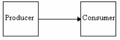
The communication graph is a graph of processes and their communication relations. A communication relationship is defined as a directed relationship, which represents message flow between a sender and a receiver process. The communication relationships are data-oriented. The communication graph is actually a data-flow diagram (DFD) which represents a network of processes that communicate through channels. A communication relationship is symbolized as an line with arrow head (►) between two processes. See figure 2.2.
Figure 2.2 shows two processes and their communication relation which represents message flow between a sender process (Producer) and a receiver process (Consumer). In this case, the producer performs sending data to the consumer.
2.3.2 Composition Graph
The composition graph shows the processes with their compositional relationships. A compositional relationship is defined as a labeled relationship between two processes whereby the label is a two-way or binary operator that expresses their compositional behavior. The compositional graph shows the processes in the same topography as the communication graph. The composition graph is control-oriented and represents a special kind of control-flow diagram that can express concurrency and non-deterministic behavior. This includes scheduling, priority and choices.
Compositional relationships in the CSP diagram are based on the CSP and CSPP operators. Thus, operator є { , , , , , , , }. Table 2.1 gives an overview of these
operators.
Operator Inverse Operator Name
Sequential Parallel
Priority parallel
Alternative
Priority Alternative
Table 2.1 Operators
Figure 2.2 Communication relation
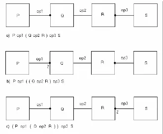
Not all of the possible relations between processes have to be shown. If all possible relations are shown, the graph is a complete composition graph. A complete composition graph of n
processes would therefore show ( n * (n – 1 )) / 2 relations. For example figure 2.4a shows three processes P, Q and R and the relations op1 and op2. Figure 2.4b shows a complete composition graph in contrast to figure 2.4a).
There exists a relation between process P and R, namely op3. Sometimes it is possible to uniquely determine the relation op3 between process P and R from the relations op1 and op2. If a relation between two processes can be uniquely determined from another path of relations between these processes then this relation is called a deduced relation.
So far we have considered the compositional relations between two processes. For a compositional relation between a process and a group of processes, we need a notion of grouping, such as using brackets, is needed. For example, P ║ ( Q → R ). For this a special composite symbol for the compositional relation is introduced, see figure 2.5.
The use of the composite is limited to one level. To extend this technique an index can be placed next to the composite symbol. When there is no index placed next to the composite symbol it implicitly means that it has index one. Figure 2.6 shows 3 examples.
Figure 2.4: a) incomplete composition graph b) complete composition graph
2.4 20-SIM
20-sim is a software tool, which can be used to model and simulate real-time systems(Broenink and Kleijn, 1999). 20-sim models are hierarchical structured and encapsulation is fully supported. 20-sim supports equations, block diagrams, bond graphs (Paynter, 1961; Breedveld, 1985), iconic diagrams and any combination of these four (ControlLabs Product B.V., 2000).
A bond graph describes a physical system as a number of physical concepts (the elements) connected by energy flows (the bonds). A bond between two elements transfers power from one element to the other. An iconic diagram uses icons which look like the corresponding parts of the physical model. These icons are also connected by energy flows (the connections). The equations behind the bond graph elements, icons and submodels are specified as equalities, this means that the variables need not be tagged as inputs or outputs yet (Broenink, 1999). The interfaces are ports, each with two variables being computed in opposite directions. For example, a resistor has one port, the variables are current and voltage. If the current is the input then the model calculates the voltage and vice versa. When a computation is made for a model, a special routine has to derive a causal form of these equations. Using this causality the equations can then we rewritten to assignments statements and have to be sorted. It then is possible that the statements of one submodel are placed between the statements of another submodel. If a CSP diagram is created for such a model, then the topography of the processes will not be the same as the topography of the submodels in 20-sim.
Both the bond graph model and the Iconic diagram model are used to model a physical system. Developing (generating) software for these models is only useful to simulate the behavior of the physical system on a computer.
In contrast, the implementation of control laws do not use energy flows. Models used for controllers contain only information processing parts. The connections between two elements are not based on energy flows but on signals (data). The model of a controller in 20-sim is therefore comparable with a communication graph.
20-sim models are hierarchical structured. The model on the top of the hierarchy is called a
mainmodel. The models on the lowest level are called elementary models, and are sets of
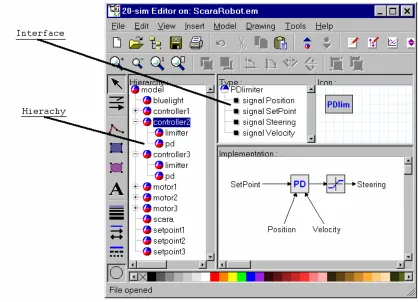
equations or assignment statements (Broenink, 1999). 20-sim shows this hierarchical structure in a tree. In figure 2.7 a 20-sim model of a robot is shown. This demo model comes with the 20-sim package. The hierarchy shows all the submodels in a tree structure. Every submodel in 20-sim has an interface. The interface specifies the ports and parameters of a submodel. The interface of the in the tree hierarchy selected submodel, (in figure 2.7
controller2) is also shown as a tree structure by 20-sim.
2.5 Tree-based Description Model
2.5.1 Introduction
The CSP paradigm offers a language to specify the behavior of software. The algebra of the CSP language is not a pleasant modeling language for developing software. The user prefers a graphical user interface and have the tool handle the mathematics. Recently, several design and specifications methods have been developed. The UML method (Douglass, 1998) is currently widely used. The research behind CTJ showed that the CSP concepts could be modeled in UML in the form of design patterns. However, describing the CSP concepts in UML does not always give a easy overview of the design (Volkerink, 2000).
The Tree-based Description Model has been developed by Eric Volkerink (Volkerink, 2000). This model is able to describe the CSP aspects visually. The CSP constructs are shown in a tree structure, like 20-sim uses for its model hierarchy and the interface of the submodels. The purpose of the tree-based description model is to integrate the CSP concept with the modeling and simulation package 20-sim. The next section gives a description of this tree-based description model.
2.5.2 Tree-based description model
Figure 2.8 shows a tree-based description model of a producer-consumer process. In this tree a hardware section and a process section can be recognized.
In the hardware section we find the elements, system ( ), processor ( ), bios ( ) and linkdriver ( ). In the process section we find the hierarchy of the execution framework and
the patterns of communication.
Hardware section
The tree always starts with a system element ( ), in figure 2.8 called Main. A system can
consist of multiple subsystem elements ( ), one or more processors ( ) and only one bios element ( ). A processor element can consist of one bios element ( ) and one custom process element ( ). This custom process element is the start of the process section. The
bios element describes the basic input-output functions of a processor or system. The bios element can have multiple child bios elements ( ) and multiple link driver elements ( ). The bios elements are introduced to structure the link driver elements.
Process section
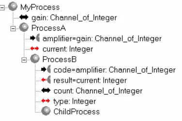
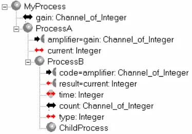
The processor element can have one custom process ( ) child. For the processor in figure 2.8 this element is called MyProcess. The custom process element can have a list of child elements. This list can be classified in four sections: (1) the process identification section, (2) the process interface section, (3) the local variable/channel declaration section and (4) the process declaration section. This is more clearly illustrated in figure 2.9.
The process identification section identifies the process. The custom process in the tree can
be folded or unfolded. If the process element is unfolded all the children of the element are shown. For large models with many custom processes, it would show to many details. For large models the user can unfold only those custom process elements he is interested in and leave the others folded.
The process interface section shows the process interface. Communication takes place using
variables and channels. In the case channels are used the process interface can consists of channel input elements ( ), channel output elements ( ) and channel pass-through elements ( ). In the case variables are used the process interface can consists of variable input elements ( ), variable output elements ( ) and variable pass-through elements ( ).
Every process interface element is specified by its local name. In figure 2.9 these are code
and result. These process interface elements are connected to a declaration element or a
process interface element that is in scope. The process interface element result is
connected to the declaration element current. The name of the declaration element is
placed after the equal sign (=) together with its type. The process interface element code is connected to the interface element amplifier.
The local variable/channel declaration section declares the local channels and variables.
These locally declared channels and variables can be used by the child process section of MyProcess. In figure 2.9 there are 4 declaration elements: gain, current, count and type.
The process declaration section forms the body of the process. It can consist of a custom
process element, a code segment or a construct process. In figure 2.9 an example of a custom
process as the body of a process is shown. The body of ProcessA consists of the custom
process ProcessB. A code segment ( ) contains the code of the process.
Figure 2.8 The four sections of the custom process element
A construct process is a composition of processes. The construct process does not have a process interface section or a local channel/variable declaration section. The only valid child processes for a construct process are process elements. There are five different construct processes: parallel, priparallel, sequential, alternative and prialternative. These are the five defined CSP compositional relationships (Hilderink, 2001). In figure 2.10 an example using parallel, sequential and priparallel construct elements is shown The tree-based description model is shown together with the pseudo occam code. The alternative and prialternative construct processes are not further discussed in this thesis.
Eric Volkerink defines also the elements: Skip, Reader, Writer and TimeSlicer in his thesis
(Volkerink, 2000). These elements and the alternative and prialternative elements are not further discussed in this thesis.
2.5.3 The Global Variable Declaration Element
Using the tree-based description model for developing software in ANSI C to run a simulation of the Linix system it became clear that a global variable can be useful. A new tree element can be created called the global declaration element ( ). In the example of software code in Appendix III-3, for example a global variable is used for the time.
In the tree-based description model these global variable declaration elements are placed between the process interface section and the local variable/channel declaration section. Figure 2.11 shows an example.
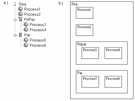
2.6 The Rectangles Graph
This graph shows a completely different view. In this graph not only the custom process elements are shown but also the parallel and sequential constructs. All these elements are shown as rectangles. If two processes run parallel they are shown next to each other within a rectangle of the tree element parallel. If they run sequentially they are shown below each
Figure 2.10 Compositions of processes: a) The construct process b) pseudo Occam code
other within a rectangle of the tree element sequential. This is best seen with an example. In figure 2.12 the same model as in the tree-based description model of figure 2.10 is shown as a rectangles graph.
This graph shows that the Process1, Process2, Pripar and Par run sequential, that Process3 and Process4 run parallel (Process3 running with a higher priority then Process4) and that Process5 and Process6 run parallel. This graph shows the
hierarchy of processes as a nesting of rectangles. A parallel construct is shown by placing the rectangles beside each other, a sequential construct is shown by placing the rectangle below each other.
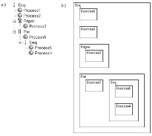
The rectangles graph can be used to make changes in the compositional relationships between processes. The user can use the mouse to move each of the rectangles. By pressing the left mouse key on a rectangle and moving the mouse, the rectangle can be moved. Every rectangle, including the rectangle representing the sequential or parallel constructs can be moved this way. The idea behind this is that when for example the rectangle of Process4
is moved and dropped, by releasing the left mouse key, just below Process5 that the tool
will then change the structure of the tree-based description model accordingly to make
Process4 sequential to Process6. The new structure is shown in figure 2.13. An
optimization routine can then be used to remove the priority parallel construct Pripar. This
construct only contains Process3 and can be removed. Placing a rectangle not below but
beside (before or after) an other rectangle would indicate that these processes should run parallel. Using this technique the sequential and parallel constructs can be manipulated. Creating a priority parallel construct can be done by first creating a parallel construct and afterwards changing this construct to a priority parallel construct.
The sequence in which the processes are shown in the tree-based description model and the rectangles graph is important for the sequential and the priority parallel construct. Because the user can easily place the rectangles below, above, left or right of another rectangle this sequence can be easily changed.
If in the model more than one processor is present then these processors are shown as rectangles next to each other. In these rectangles the processes running on these processors are shown. An example is shown in figure 2.14.
Selecting a process for example Process1 and moving it to the processor Pentium2
would indicate that the process should be allocated on this processor. In an ideal case the tool should show the communication relationships between the processes and the available link drivers between the processors. When the user moves a process to another processor the tool should then let the user choose which link driver should be used for which communication relationship.
Figure 2.14 Three processors in a rectangles graph
2.7 The Deployment Graph
The rectangles graph shows in principle all processes and the (priority) parallel and sequential constructs. The deployment graph shows only the available processors and those processes which are candidates to be allocated on another processor. The always has at least one processor in its design. The deployment graph would then show the processor(s) and a list of processes which can then be allocated on a processor. The deployment graph is in fact a compact representation of the rectangles graph.
2.8 Outline
3 USE-CASE
3.1 Introduction
The use-case presented here is the development of a controller for the Linix system. The Linix system is described in section 3.2. The method used for developing the controller is as follows: (1) Physical Systems Modeling: In section 3.3 a model of the Linix system is created and simulated in 20-sim. (2) Control law design: In section 3.4 a controller is designed using block diagrams, and simulated in 20-sim. (3) Embedded control systems implementation: In section 3.5 the composition graph is used to add concurrency to the design.
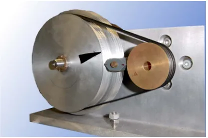
3.2 The LINIX system
The Linix is a system build at the Engineering Control Laboratory (figure 3.1). It is used for educational purposes. It consists of an voltage controlled current output amplifier, an electromotor and two pulleys which are connected through an elastic band (a flexible transmission belt).
The amplifier has a ± 5 Volt input voltage range. The output current is between ± 1.33 Ampere. Both pulleys have a certain inertia. The positions of both pulleys are measured by optical encoders. These encoders have a resolution of 2000 steps/revolution. The output of these optical encoders are converted into a 16 bit binary representation.
Figure 3.1 The LINIX system
3.3 Physical Systems Modeling
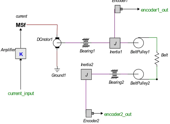
A model of the LINIX system is created in 20-sim using iconic diagrams (figure 3.2). The connections between the displayed icons are energy flows. The model has two output signals, encoder1_out and encoder2_out, and one input signal, current_input. The icons Encoder1, Encoder2 and MSf are responsible for converting energy flows to signals or vice versa.
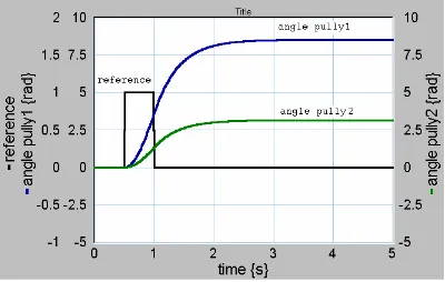
To simulate this model with 20-sim we need to add a signal source. The source is a pulse generator and gives an output of amplitude 1 between 0.5 and 1 second. The output of the signalgenerator is connected to the input signal current_input of the Linix model.
The simulation is shown in figure 3.4. In this simulation three signals are shown: 1. Reference, this is the output of the signal generator (a pulse).
2. Angle pully1, this is the angle of pully1 in radian. 3. Angle pully2, this is the angle of pully2 in radian.
SignalGenerator
Linix
Figure 3.2 Linix model in 20-sim
Figure 3.3 Signal source and Linix
current_input
encoder1_out
encoder2_out MSf
current
DCmotor1
Ground1
Bearing1
J
Inertia1 BeltPulley1
Bearing2
J
Inertia2
BeltPulley2
K
Amplifier
Belt Encoder1
3.4 Controller Design
3.4.1 The controller
For this example a P-controller is used. The reference signal is the angle of the second pulley. A value of 1 V of the reference means that pulley2 has to rotate to a position of 1 rad. As feedback signal the output signal encoder1_out of the Linix model will be used.
Figure 3.5 shows the Linix system with controller and reference, and the data-flow diagram of the controller.
a) b)
The output of the reference is connected to the input signal reference of the controller.
The output signal encoder1_out of the Linix model is connected to the input signal encoder1 of the controller. The output signal control of the controller is connected to
the input signal current_input of the Linix model.
The encoder has a resolution of 2000 steps per revolution. The amplification factor of submodel Encoder_correction is therefore: (2 * pi) / 2000. The feedback signal must
be corrected for the transmission ratio between the two pulleys, because the feedback signal is taken from the encoder on the first pulley while we want to steer the second pulley. For this correction the submodel Encoder_correction is used. The amplification factor in
this submodel is 0.37037037. The proportional gain of the submodel Kp has the value 0.5.
Figure 3.4 Simulation of Linix with pulse as reference
reference
encoder1 K
Transmission
K
Encoder_correction
K
Kp
control
Figure 3.5: a) The Linix system with controller and reference, b) the controller
Linix
reference
3.4.2 Safety Layer
The output of the encoders is converted to a binary 16 bit representation. This means that the value of the encoders must not exceed ± 215 – 1. To make sure that these values will not be
exceeded, a safety layer will be added. When for example a constant signal is added to the input signal current_input of the Linix model then the electromotor will start running
with a constant speed. The output of the encoders will constantly rise until they reach the value of 215 – 1. In figure 3.6 this is shown by the line from A to C. After that point the value will instantly drop to the value of -215. The safety layer contains a P-controller with a low proportional gain. This P-controller calculates the control signal which is needed to steer the output of the encoder slowly to a maximum value. If this control signal is used the
encoder output would follow the line A – B – D. The safety layer will use this control signal as a maximum value for the signal send to the Linix system. The maximum value of 32000 is used and not 215-1 to allow some overshoot. Figure 3.7 shows the model of the system including the safety layer and the submodel SafetyLayer. The output of Encoder2 of
the Linix system is always smaller then the output of encoder1, because the two pulleys
have a different diameter. The submodel Gain1 in the submodel SafetyLayer
compensates this difference.
a) b)
Both the Safety and Choice submodels are equation submodels. See figures 3.8 and 3.9.
Table 3.1 lists the connections between the input signals and the output signals.
Figure 3.6 Encoder output
Figure 3.7 a) The Linix system with safety layer, b) The SafetyLayer submodel
Linix
Reference
Controller SafetyLayer
encoder2 Controller_in
Control
Choice
Safety K
ports
signal in encoder_in; signal out safe_value; signal out safe_code; end;
parameters
real K = 0.0001;
real encoder_start_max = 20000; real encoder_abs_max = 32000; equations
if encoder_in > encoder_start_max then
safe_value = (encoder_abs_max - encoder_in) * K; safe_code = 1;
else
safe_code = 0; end;
Figure 3.8 The submodel Safety
ports
signal in controller_in; signal in safe_value; signal in safe_code; signal out control_value; end;
equations
if safe_code > 0.5 then
if controller_in < safe_value then
control_value = controller_in; else
control_value = safe_value; end;
else
control_value = controller_in; end;
Figure 3.9 The submodel Choice
From To
Submodel Signal Submodel Signal
Linix encoder1_out Controller encoder1
encoder2_out Safety encoder_in
Reference Output Controller Reference
Controller control Choice controller_in
Choice control_value Linix current_input
Safety save_value Choice save_value
save_code save_code
Table 3.1 The connections of the input and output signals
If the encoder output reaches a value of 20000 then the submodel Safety calculates the
maximum value of the control signal save_value and sets the output signal safe_code
to one. The submodel Choice will then calculate the minimum value of the control signal from the controller controller_in and the save_value of the submodel Safety.
lower then 20000, the submodel Choice will use then use the control signal from the controller controller_in to steer the Linix model.
3.4.3 Simulation
This controller can be verified by simulation. For this an experiment was setup in 20-sim. As a reference (source) a cycloid function is used. The result of this experiment is shown in figure 3.10. The simulation shows that between the points A and B the control value of the safety layer is used.
3.5 Embedded control systems implementation
3.5.1 Model Enhancement
Most of the (sub)systems in 20-sim are I/O-SEQ, meaning that they first read all their input before giving an output. When these submodels are converted into software, each submodel can in fact be represented as a software routine. Figure 3.11 shows the tree-based description model, the communication graph and the composition graph of the Linix system as shown in figure 3.7a, in case all the processes are run sequentially.
Not all the possible relations in the composition graph are shown in this example. The example shows a deduced composition graph. This means that every relation between two processes which is not shown can be deduced from the graph. For example the relation between Controller and Linix is a sequential relation from Controller to Linix.
Figure 3.11 The Linix system a) Tree-based description model
b) Communication graph
In a design it is not necessary to work with a complete composition graph. The designer is only interested in those relations which are essential for his design. If the designer wants process SafetyLayer run parallel to the other processes, then he will have to define all
the relations to the process SafetyLayer as a parallel composition. The resulting graph is
shown in figure 3.12 together with the tree-based description model. In figure 3.13 the composition graph of the same model is shown using the composite symbol (●).
Figure 3.12 The Linix system with submodel SafetyLayer running in parallel
a) Tree-based description model
3.6 Code Generation
The software tool Topo is used to generate software for the developed controller. This tool
was developed for this assignment and is described in chapter 4 and 5.
The software tool Topo was used to generate the software. For the controller as shown in figure 3.11 ANSI C code is generated. This code can be found in appendix III-1. For the controller as shown in figure 3.12 Java code using the CTJ package is generated. Appendix III-2 shows the generated Java code for the process Main. Only the structure of the code and the interfaces are generated, the processes do not contain a code block.
In Appendix III-3 the results of a 20-sim simulation for the system as shown in figure 3.5 is compared with the results of the generated software from a tree-based description model of the same system.
3.7 Outline
This chapter described a use-case for the development of a controller for the Linix system. The tree-based description model, communication graph and the composition graph of the developed controller were shown. The generated software for this model can be found in appendix III. The code is generated using the Topo. This tool will be described in the next two chapters.
4 The Design of Topo
4.1 Introduction
In this chapter the development of the design tool, called Topo, will be described. The
program is written in Microsoft Visual C++. In section 4.2 an overview of Topo is given. The tool can be divided in five parts, the database, the select view, the tree structure view, the topographic view and the code generator. In the sections 4.3 to 4.7 these parts are described.
4.2 Overview
The structure of the tool is shown in figure 4.1.
From this figure we can divide the tool in 5 parts:
1. The database contains the information shown in the tree structure view and the
topographical view.
2. The select view shows the input/output variables/channels of a process and can be used
by the user to set how much detail the tree view is shown. The user also uses this view to define which of the four possible topographic views are shown.
3. The tree structure view shows the data as a tree. It shows the tree-based description
model (Volkerink, 2000). This view also takes care for the interaction with the user for entering new data to, modifying data or removing data from the database. For entering new data, a syntax rule checker is used.
4. The topographical view shows the information as a graph. There are four different
graphs possible, the communication graph, the composition graph, the rectangles graph and the deployment graph.
5. The codegenerator performs the conversion from the database contents to software code.
Currently the languages ANSI C and Java are supported.
In the next sections these five parts will be discussed.
4.3 The Database
For implementing the database there are basically two main alternatives:
• Using an external database (e.g. Microsoft Access).
• Create the database internally in memory.
An external database has the advantage that existing tools can be used to test and read the database. Most existing databases have built-in safeguards to maintain the integrity of the database. This can be of great help during the development of the tool. The disadvantage is that the tool has to access the database using SQL. Several years of experience in programming databases have shown that it is not always easy to implement queries for databases.
Implemented the database internally in C++ means that the database will be in memory constantly. Because a object-oriented language is used to implement the tool a good separation of the database object and the other parts of the tool can be created, using features like data protection and information hiding. In addition, the Microsoft Foundation Classes makes it very easy to read and write internal data to persistent media. As a result it was decided to implement the database internally as a C++ object.
Unique ID
label Type (enumerated)
Parent (pointer to)
Next_sibling (pointer to)
1 Main System Null Null 2 Processor Processor Main Null 3 PCMain1 Custom Null Null 4 channel Channel PCMain1 Par
5 par Par PCMain1 Null
6 Producer Custom par Consumer 7 out Channelout Producer Object 8 object Variable Producer Code 9 Code Code Producer Null 10 Consumer Custom par Null 11 in Channelin Consumer Object 12 object Variable Consumer Code 13 Code code Consumer Null
4.4 The Select View
The topographic view can show one out of four different graphs. The user has to have a way to indicate which graph he wants to see. There are three methods which can be used for this:
1 Keyboard, a special keystroke is used for each of the four graphs. 2 Menu option, have the user use the menu system.
3 Buttons, four (radio) buttons are placed inside the program window, one for each graph. Because the selection of which graph is shown is an important feature of the program the third option, using four radio buttons, is chosen.
Erik Volkering developed a program for his thesis which shows the tree-based description model (Volkerink, 2000). Using this program it became clear that for models with many interface elements it was difficult to see the hierarchy of the processes clearly. An option to show the tree-based description model without the interface elements would solve this. A disadvantage of this is, that the interface is no longer visible. 20-sim shows the interface elements of the selected submodel, in a separate window. By implementing such a window in Topo, the user can view the hierarchy of processes in a compact manner and at the same time see the interface elements of one process.
Figure 4.2 Tree-based description model of a producer-consumer system
In figure 4.3 an example of the select view is shown.
The leftmost part of this view shows the interface elements of the selected process in the tree structure view. If the selected element in the tree structure view is not a process element then the parent process of the selected element is shown with its interface elements.
The middle part of this view contains three radio buttons.
1 20-sim, the tree-based description model in the tree structure view is shown comparable with the software package 20-sim. For Topo this means that only the system elements and process elements are shown. See figure 4.4 a).
2 Compact, besides the elements shown in the 20-sim options, this option also shows the processor elements, the codeblock elements and the elements for the composition relations like parallel, priority parallel and sequential. See figure 4.4 b).
3 Extended, all the elements in the tree-based description model are shown in the tree structure view. See figure 4.4 c).
In the rightmost part, the user can select which graph (Communication graph, Composition graph, Rectangles graph or Deployment graph) is shown in the topographic view.
4.5 The Tree Structure View
Because this research is a continuation of the work of Erik Volkerink, the design of this view was based on his design of the tool Embedded (Volkerink, 2000). This view shows the
tree-based description model which is discussed in section 2.5. Editing a model in Topo can only be done by changing the tree-based description model. The model cannot be changed in the topographic view. In 20-sim this is different. Editing of a model in 20-sim can only be done in the topographic view.
To enter new elements in the design the menu structure is used. Before the user can select a menu item to enter a new element, the syntax rules checker first checks which type of elements can be entered. The same syntax rules as used in the program Embedded are
Figure 4.3 The select view
implemented in Topo. For example, after a variable declaration element ( ), one is not allowed to add any child. The syntax rules are described in Appendix II.
4.6 The topographical view
The topographic view can show four different graphs. These graphs use the contents of the database to create the graphs. Changing the contents of the database is done by the tree structure view.
1. The communication graph shows the processes and their communication relationships. This graph should be comparable with the way 20-sim shows a data-flow diagram. The processes are therefor shown as rectangles and the relationships as line with a arrow head(►). When there is more then one relationship between two processes, these relationships have to be shown separately. In figure 4.5 two ways to archive this are shown.
Because 20-sim uses the intermediate points as shown in figure 4.5b) this method is also used in Topo. To minimize the programming effort only one intermediate point will be supported.
2. The composition graph shows the processes and their composition relationships. This graph uses the same topography for the processes as the communication graph. The processes are shown as rectangles. The routine used for showing these rectangles in the communication graph can be used for the composition graph. The relationships are shown as lines with a label which indicates the type of the composition { , , , ,
}. The alternative relationships { , , } are not supported by Topo.
Showing all the possible relations between all processes is not necessary. The tool should initially make a selection of all possible relationships and show these. The user should then be able to indicate which relationships he wants to see. The most important relationships to show initially are the relationships between the child processes of a parallel or sequential construct. The sequence in which these child processes are placed in the tree-based description model indicates the direction of the sequential and priority parallel composition. Figure 4.6 gives an example.
Figure 4.5 two ways to show two relationships between two processes
Only the relationship between Process1 and Process2 and the relationship between Process2 and Process3 are shown. A problem occurs if one of these child
processes is a parallel or sequential construct. Such a construct is not shown as a process in the graph. For this situation the composite symbol (●) has to be used. Figure 4.6 shows the use of this composite symbol if the Process2 of figure 4.5 is replaced by a parallel construct.
3. The rectangles graph shows the processes as rectangles. The rectangles for child processes are placed inside the rectangle of the parent process. For a sequential construct the child processes are placed below each other and for a parallel construct the child processes are placed next to each other. The size of the rectangle for the parent process has to be changed so that all the child processes will fit into this rectangle.
The rectangles graph shows the hierarchy of the processes in the tree-based description model. Because the number of levels in the tree-based description model can be large, the number of levels shown in the rectangles graph have to be limited. In the select view the user can be set the number of levels the rectangles graph will show.
The rectangles graph can be used to make changes in the compositional relationships between processes. This can be done by using the mouse to move the rectangles and ‘drop’ them on their new position. The structure of the tree-based description model can then be changed to this new situation. Because the rectangles graph shows the processors as rectangles, this graph can be used to allocate processes on another processor.
4. The deployment graph shows the processors which are defined in the tree-based description model as rectangles places next to each other. Inside these rectangles, the processes that run on these processors and which are candidates to be allocated on another processor are shown as rectangles. These processes can then be moved (‘drag and drop’) to another processor. The deployment graph is in effect a more compact version of the rectangles graph.
If a process, that communicates with another process on the same processor, is allocated on another processor, then the communication has to take place using a linkdriver. To make this visible to the user, the communication relationships between the processes and the available linkdriver on each processor should be visible in the deployment graph. The deployment graph should let the user choose which linkdriver should be used.
4.7 The Code Generator
The code generator uses the contents of the database to generate software code. To develop the code generator two alternatives were considered.
1 Design a general algorithm for code generation and use a separate database for the language dependency.
2 Create a code generation algorithm for each language.
Using the first alternative makes adding a new target language relatively easy. The disadvantage, however, is that because of the differences between the target languages the general algorithm for code generation is not easy to develop. Also the database for the language dependency can become very complex. The advantage of the second alternative is that the code generator can be customized for a specified target language.
The current implementation of the code generator is based on a separate code generator for each target language. Currently two code generator algorithms are implemented. One for ANSI and one for Java. The code generator for Java uses the CTJ package (Hilderink et al.,
1999). The code generator for ANSI C generates the code using a sequential framework. This generator can easily be enhanced to make use of the CTC software package (Hilderink, 1999).
4.8 Outline
5 Users Manual
5.1 Introduction
In this chapter a users manual of Topo is given. The tool is based on the tree-based description model. This model shows the hierarchy of the processes in a tree structure. In figure 5.1 a screen view of the program is shown. The screen view shows the tree structure view, the select view and the topographic view.
The menu structure of Topo is described in section 5.2. The tree structure is described in section 5.3. This section also describes the editing of the model. The select view is described in section 5.4. The topographic view can show four different graphs, the communication graph, the composition graph, the rectangles graph and the deployment graph. These are described in the sections 5.5 through 5.8. In section 5.9 the use of the semantic rules checker, which is used before generating the software, is described and in section 5.10 three option dialog boxes are described.
5.2 Menu Structure of Topo
The menu structure is shown in figure 5.2. Only the menu items specific for Topo are discussed. The others are standard for window applications.
For entering new elements in the tree structure the Add Child or Insert Sibling submenu of the Edit submenu has to be selected. The Insert Sibling submenu has the same sub options as the Add Child submenu. Not all menu items in these submenu’s can be selected. The elements Alternative, PriAlternative, Reader, Writer, Skip, Stop, TimeSlicer, Input Guard, Output Guard, Skip Guard and Timeout Guard are not supported by Topo and are currently disabled. The entering of new elements to the model is further discussed in section 5.3.
* The Insert Sibling submenu has the same sub options as the Add Child submenu.
The submenu Options in the submenu View has three menu items, General Options, ANSI C and Java. These menu items each start a dialog box for options. These dialog boxes are further discussed in section 5.11.
The submenu Build contains the submenus Check Code and Generate Code. These are used for running the semantics rules checker (section 5.9) and for starting the code generators (section 5.10).
5.3 The Tree Structure View
This view shows the tree-based description model which is discussed in section 2.5. The user can delete an element from the model, modify an existing element or add an element to the model.
Tree elements can be deleted from the tree by selecting the element, using the mouse or the arrow keys of the keyboard (↑, ↓), and pressing the ‘Delete’ key. The tool will instantly remove the selected element and all its children from the tree. The tool will not ask for confirmation and a ‘redo’ facility is not present.
Modifying existing elements takes place by ‘double-clicking’ in the tree on the element. Topo will then show a dialog window in which the user can modify the item belonging to the
element. The tool will use the same dialog window as for new tree elements. The title of this window however begins with the word ‘Modify’ instead with the word ‘New’.
For entering new elements for the tree structure the menu is used. Not all menu items can be selected. The syntax rules checker first checks which type of elements can be entered. For example, a system element can have only one bios element. The syntax rules checker will first check if the system element has a bios element before enabling the Bios menu item. If there is a bios element present then the menu item for bios will be disabled. In appendix II, a table can be found with the rules which the syntax rules checker enforces. For entering the data for the tree elements seven dialog windows are used for the following groups of elements:
1. Subsystem ( ), bios ( ), processor ( ) and linkdriver ( ) 2. Declaration of variable ( ), channel ( ) and global variable ( ) 3. Parallel construct ( ) and priority parallel construct ( )
4. Custom process ( )
5. Variable input ( ), variable output ( ), channel input ( ) and channel output ( ) 6. Code segment ( )
7. Sequential construct ( )
These dialog windows are shown in the section 5.3.3 through 5.3.9. The Producer Consumer example of figure 5.3 will be used to show each of these dialog windows.
Each of the dialog windows has three items in common:
1. Name, the name is used as the label for the tree element in the tree structure.
2. Description, this is a text field where a description for the tree element can be
entered. The code generator will generate comments in the source using this description. However not all tree elements are treated as such.
3. Sequence, this field gives the user the ability to change the sequence of the elements
in the tree structure. This is explained in section 5.3.1.
5.3.1 The sequence of the tree-elements
The tool will in principle append a new child to the already existing children. The sequence in which they are shown is the same as the sequence they are entered. The only exception is the sequence of the sections of the custom process element. The sequence of the five sections of the custom process (process identification, process interface, global declaration, local declaration, child process) cannot be changed. The user can change the sequence of the tree elements within one section. Also the sequence of the children of a construct element (for example parallel, sequential) can be changed by the user. The tool will not change the sequence directly. The sequence will be changed during the loading the file from the disk. Therefore after setting all relevant sequence numbers, the data has to be saved to disk and reloaded before the changes take effect.
5.3.2 Dialog 1: Subsystem, bios, processor and linkdriver
This dialog window is used for the elements subsystem ( ), bios ( ), processor ( ) and linkdriver ( ). The window contains only the three common items: Name, Description and Sequence.
5.3.3 Dialog 2: Declaration of variable, channel and global variable
The dialog window is shown in figure 5.5. This dialog window is used for the elements channel ( ), variable ( ) and global variable ( ). The window contains the three common items: Name, Description and Sequence.
The other items in the window:
• Type, this item defines the type of communication. Currently there are four types of
communication defined: integer, double (floating point), character and boolean.
• Initial, for a global variable ( ) or a variable ( ) it can be useful to set a initial value.
For a channel declaration this element is ignored.
• Constant, for a global variable ( ) or a variable ( ) it can be useful to define the
variable as a constant. For a channel declaration this element is ignored.
• In, when a input variable cq input channel of a child process is connected to this
declaration element then the item in contains the name of this child process and the name
of the input variable cq input channel. In figure 5.5 the name of the child process is
TwoConsumers and the name of the input channel is in1.
• Out, when a output variable cq output channel of a child process is connected to this
declaration element then the item out contains the name of this child process and the
name of the output variable cq output channel. In figure 5.5 the name of the child process is Producer and the name of the input channel is out1.
5.3.4 Dialog 3: Parallel and priority parallel construct
This dialog window is used for the parallel ( ) and priority parallel ( ). The window contains the three common items: Name, Description and Sequence.
Figure 5.5 Dialog 2: channel ( ), variable ( ) and global variable ( ).
There is one other item in the window:
• Priority, when the element is a priority parallel construct then the checkbox is set.
Changing a parallel construct to a priority construct can be realized by setting this checkbox.
5.3.5 Dialog 4: Custom process
This dialog window is used for the custom process ( ). The window contains the three common items: Name, Description and Sequence.
There is one other item in the window:
• Nr of Iterations, this item is used by the code generator to decide whether a for-loop or a
while-loop has to be generated. This loop is placed around the child process elements of this element. There are three possibilities:
1. The value of the item is equal to zero: a while ( true ) loop will be generated. 2. The value of the item is equal to one: no loop is generated.
3. The value of the item is greater then one: a for loop is generated.
5.3.6 Dialog 5: Channel/variable input/output
The dialog window is shown in figure 5.8. This dialog window is used for the variable input ( ), variable output ( ), channel input ( ) and channel output ( ). The window contains the three common items: Name, Description and Sequence.
There is one other item in the window:
• Connected, A channel or a variable input/output element has to be connected with a
channel declaration element or a channel interface element from the parent process. The tool will select all the available possibilities and show them in a selection list. The value ‘not_connected’ is added to