Effective Image Restorations Using a Novel Spatial Adaptive Prior

(1)

Volume 2010, Article ID 508089,10pages doi:10.1155/2010/508089

Research Article

Effective Image Restorations Using a Novel Spatial Adaptive Prior

Yang Chen,

1, 2

_{Yinsheng Li,}

1, 2

_{Yingmei Dong,}

3

_{Liwei Hao,}

2

_{Limin Luo,}

1

_{and Wufan Chen}

2

1_{The Laboratory of Image Science and Technology, Southeast University, Nanjing 210096, China} 2_{The School of Biomedical Engineering, Southern Medical University, Guangzhou 510515, China}

3_{Cadre Reset Institute, The Joint Logistics Department, Chengdu Military Region, Chengdu 610083, China}

Correspondence should be addressed to Wufan Chen,[email protected]

Received 20 October 2009; Revised 29 December 2009; Accepted 16 February 2010

Academic Editor: Liang-Gee Chen

Copyright © 2010 Yang Chen et al. This is an open access article distributed under the Creative Commons Attribution License, which permits unrestricted use, distribution, and reproduction in any medium, provided the original work is properly cited.

Bayesian or Maximum a posteriori (MAP) approaches can eﬀectively overcome the ill-posed problems of image restoration

or deconvolution through incorporating a priori image information. Many restoration methods, such as nonquadratic prior Bayesian restoration and total variation regularization, have been proposed with edge-preserving and noise-removing properties. However, these methods are often ineﬃcient in restoring continuous variation region and suppressing block artifacts. To handle this, this paper proposes a Bayesian restoration approach with a novel spatial adaptive (SA) prior. Through selectively and

adaptively incorporating the nonlocal image information into the SA prior model, the proposed method eﬀectively suppress

the negative disturbance from irrelevant neighbor pixels, and utilizes the positive regularization from the relevant ones. A two-step restoration algorithm for the proposed approach is also given. Comparative experimentation and analysis demonstrate that, bearing high-quality edge-preserving and noise-removing properties, the proposed restoration also has good deblocking property.

1. Introduction

1.1. Problem Formulation. As one of the most classical linear inverse problems, image restoration has its wide applications in remote sensing, radar imaging, tomographic imaging, microscopic imaging, astronomic imaging, digital photography, and so forth [1–4]. For linear and shift-invariant imaging systems, the transformation from f tog

is well described by following additive linear degradation model [3,4]:

g=A∗f +ε, (1)

where g, f, and ε represent, respectively, the degraded observed image, the original true image, and the corrupting white Gaussian noise with varianceσ2_{. Point-spread function}

(PSF)Ais the imaging system and∗is the linear convolution operator. Throughout this paper we assume that the degra-dation model PSFAand noise varianceσ2_{are known for they}

could be numerically estimated or calibrated.

Based on the Gaussian statistics of the additive noise, maximum log-likelihood (ML) restoration method could be

applied to find the least-squares estimation of f. However, such ML restoration method often leads to unacceptable restoration solutions due to the ill-posedness of the inverse problems. Small changes in the data due to noise can cause large changes in the solution, and the knowledge of the degradation model is not suﬃcient to determine a restoration result with acceptable accuracy [2–5].

(2)

We can build following posterior probability P(f | g) for image restoration

Pf |g∝Pg| fPf, (2)

Pg| f=expLg,f=exp

−1

2κg−A∗f

2

,

(3)

Pf=Z−1×exp−αUf=Z−1×exp

⎛ ⎝₋_α

j

Uj

f

⎞ ⎠_.

(4)

Here,P(g | f) is the likelihood distribution andP(f) is the prior distribution. The partition functionZis a normalizing constant.U(f) is the prior energy function, andUj(f) is the

notation for the value of the energy functionUevaluated on the fat pixel index j.α is the global hyperparameter that controls the degree of the prior’s influence on the image f. The energy functionU(f) in (4) attains its minimum and the corresponding prior distribution (4) attains its maximum when the image meets the prior assumptions ideally. So from (2)–(4), we can build the log-posterior energy function as

logPf |g=Lg,f−αUf

= −1

2κg−A∗f

2₋ α

j

Uj

f. (5)

The reconstructed image f can be obtained through itera-tively maximizing functionψ(f).

The simple and widely used quadratic membrane (QM) prior or the Tikhonov L2 regularization, which smoothes both noise and edge details equally, leads to a linear inversion process and tends to produce an unfavorable oversmoothing eﬀect [5].

To solve this oversmoothing problem, many edge-preserving Bayesian restoration methods were proposed in the past twenty years. We generalize them into three main classes: wavelet Bayesian restoration, Bayesian restoration with nonquadratic prior energies, and Bayesian restoration with total variation (TV) prior/regularization.

Wavelet complexity regularization restorations, using a multiscale stochastic prior model, have also been proposed for edge-preserving restoration [8–11]. Priors based on wavelet decompositions and heavy-tailed pdfs along with the EM restoration algorithm have been proposed in [10]. These wavelet regularization methods rely on statistical modeling of the distribution of wavelet coefficients and strategy of coefficient thresholding. We choose not to include the comparison of wavelet regularization methods in this paper for the consideration that they can also be reinterpreted as some wavelet domain forms for Wiener filters, TV variational methods, or some Tikhonov regularization procedures [11]. Edge-preserving priors with nonquadratic energies were also proposed to preserve edge details by assuming a nonlin-ear inverse-proportional relationship between the existence of edges and intensity differences [5,12,13]. The weighting matrices in nonquadratic prior Bayesian restoration preserve edges by turning offor suppressing smoothing at appropriate locations.

Another impressive recent advance in this area is the total variation- (TV-) based image restoration algorithms [7,14,15]. This kind of approach can also be viewed as TV prior withthe half-quadratic regularizationprior energy. The inherent idea of TV methods describes the target images as consisting largely of zero-gradient regions interspersed with occasional strong gradient transitions. With no enforced global image continuity, TV prior restorations often demon-strate good edge-preserving property.

The nonquadratic priors aim to preserve edges through determining the regularization degree on each pixel based on the intensity-diﬀerence information within a local fixed neighborhood. The regularization information of TV prior also comes from the local neighboring intensity gradients. Limited by local prior information within local neighborhoods, these edge-preserving approaches cannot cope well with realistic complicated images, and tend to produce blocky artifacts around continuous edges [16–21].

1.2. Existing Solution and Our Proposed One. A more eﬃcient edge-preserving restoration model should be more adaptive to the characteristic structure of the image to avoid or suppress the unfavorable blocky artifacts. In the past twenty years some spatially adaptive techniques were proposed to in this way.

In this way, a line-process [5] or doubly stochastic MRF model [22] has been proposed. Bouman and Sauer proposed a generalized Gaussian MRF prior model with a power parameter controlling the background smoothness and the edge sharpness in the restored image. However, using line elements adds to the complexity of the problem by increasing both the dimensionality of the required optimization and the complexity of the parameter estimation procedure.

In [16], Mignotte proposed an adaptive region-based edge-preserving regularization term, which applies a local smoothness constraint to the preestimated constant-valued regions by a two-level MRF model. The first level is a low-level prior model used in the segmentation procedure, and the second prior model exploits the segmentation result (a partition into regions extracted from this segmentation map) as a parameter for the resulting restoration. And in a similar way but with a different application, Yu and Fessler devised a boundary-based Bayesian method for transmission tomography after level-set segmentation [23]. Such boundary or region-based methods rely heavily on the segmentation operations whose effect in different images is unpredictable and parameter dependent.

(3)

In this article, based on the work in [24] and our previous tomographic work [19–21], we propose a spatial adaptive Bayesian restoration approach. This new restoration approach utilizes a spatial adaptive (SA) prior, which exploits the global connectivity and continuity information in the objective image. It works by adaptively including the useful relevant neighbor pixels and excluding the negative irrelevant ones within a large prior neighborhood. The proposed restoration has good noise-removing and edge-preserving properties, and, especially, it can eﬀectively restore contin-uous regions with much less blocky artifacts.

InSection 2, a review of the conventional prior model and the theory for the proposed SA prior model are both illustrated. In Section 3, we give the iterative restoration algorithm for the proposed approach. In Section 4, we perform restoration using diﬀerent methods under the pro-gramming environment of hybrid Matlab and C language. Relevant visual and quantitative comparisons are also shown. Conclusions and plans for future work are given inSection 5.

2. Prior Model

In this section, after providing a review of the conventional prior model, we introduce the theory for the proposed SA prior model.

2.1. The Traditional Prior Model. Conventionally, the value ofUj(f) is commonly computed through a weighted sum of

potential functionsvof the diﬀerences between pixels in the neighborhoodNj:

Uj

f=

b∈Nj wb jv

fb−fj

. ₍₆₎

Generally, diﬀerent choices of the potential functionv

lead to diﬀerent priors. The prior is the familiar space-invariant QM prior when the potential function has the form

v(t)=t2_/_2.

Edge-preserving nonquadratic priors could be chosen by adopting a nonquadratic potential function forv, such as the Huber potential function:

v(t)=

⎧ ⎪ ⎪ ⎪ ⎨ ⎪ ⎪ ⎪ ⎩ t2

2, |t| ≤γ,

γ|t| −γ2

2, |t|> γ,

(7)

whereγ is the threshold parameter [5,13,16]. Such edge-preserving nonquadratic prior preserves the edge informa-tion by choosing a nonquadratic potential funcinforma-tion that increases less as the diﬀerences between adjacent pixels become bigger. Weight wb j is a positive value that denotes

the interaction degree between pixel b and pixel j. And in traditional prior models, it is simply considered to be inversely proportional to the distance between pixel b and pixel j. So on a square lattice of image f, in which the 2D positions of the pixelband pixel j(_{b /}=j) are, respectively, (bx,by) and (jx,jy),wb jis usually calculated by the geometric

distance 1/

(bx−jx)2+ (by−jy)2 or some other simple

forms. Here, for traditional prior models, we illustrate two widely used normalized weighting maps for eight-element neighborhood and four-element neighborhood:

(1) (1/(4×1 + 4×1/√2))×

1/√2 1 1/√2 1 0 1

1/√2 1 1/√2

(2) (1/(4×1))×

1 1 0 1

1

Restorations using Total Variation (TV) prior or regular-ization often take prior energy as follows:

UTV

f=

j

Δhjf

2

+Δvjf

2

, ₍₈₎

where Δh

j and Δvj are linear operators corresponding to

horizontal and vertical first-order diﬀerences at pixel j, respectively [7,14,15]. This TV prior energy given by (8) favors images with bounded variation without penalizing possible discontinuities since both smooth and sharp edges have the same TV prior energy.

2.2. The Proposed SA Prior Model. Objects in most images have edges with coherently varying pixel intensities. Pixel-scale intensity differences alone are insufficient to charac-terize objects of multiple scales fully. Traditional quadratic priors, nonquadratic priors, and TV prior can only provide fixed local information for image restoration. Through an averaging alike effect the local QM prior or Tikhonov regularization is prone to produce an unfavorable over-smoothing effect to smooth out both noise and details. And the edge-preserving nonquadratic and TV priors, although able to preserve some edge information, tend to produce unfavorable blocky artifacts or false edges because of the disturbance of noise. In [22], we find that simply enlarging the prior neighborhood of local prior is ineffective in improving restoration.

Thus continuous texture information within a larger scale should be used to discriminate image information from singularities or noise. This laid the basis of the proposed method. In the building of the proposed SA prior model, a large nonlocal neighborhood N is used to incorporate geometrical configuration information. Other than calculated as the Gaussian decreasing function of the diﬀerence between the two square comparing neighborhoods as the methods in [19], the weightwb j for the new selective

nonlocal prior is set to be a 1-0 binary function which classifies all pixels in neighborhoodNinto two classes—the neighbors relevant to the center pixel j and those not. Only the relevant ones are picked out for the SA prior. The value ofwb j is set to be 0 or 1 when the computed distancedb j is

greater or smaller than a set thresholdδ.

Thus, the chosen relevant pixels in the SA prior neighbor-hood for each center pixeljare not fixed. Both the numbers and positions of the relevant pixels in neighborhood N

(4)

(a) (b) (c)

(d)

Figure1: Illustrations of the weight distributions of the adaptive neighborhood system for the proposed SA prior model. The sizes of neighborhoodsNandnare 31×31 and 7×7, respectively. (a) The weight factorswb jare distributed in the direction of the straight edge line

when the centered pixeljis in a straight alike configuration. (b) The weight factorswb jare distributed in the direction of the edge line when

the centered pixeljis in an oblique edge. (c) The weight factorswb jare adaptively distributed along the pixels in the same structures when

the centered pixeljis in some special structure. (d) The weight factor distributions for the three centered pixels in the two edge regions and the background region, respectively, are shown.

spatial properties of the objective image. The building of the proposed SA prior can be formalized as follows:

USA

f=

j

Uj

f=

j b∈Nj

wb j

fb−fj

2_Nr

j

,

(9)

wb j =

⎧ ⎨ ⎩

1, disb j ≤δ,

0, disb j > δ,

(10)

disb j=nb

f−nj

f2

E= l

fl∈nb−fl∈nj 2

, (11)

nb

f=fl:l∈nb

, (12)

nj

f=fl:l∈nj

. (13)

Here,USAis the energy function for the proposed SA prior. wb j, which represents the classification of the neighbor pixels

in the search neighborhoodNj, can be computed via (10)–

(13).|Nrj|, the number of neighbor pixels with nonzerowb j

in the neighborhoodNj, can function as a normalized factor

of hyperparameter βfor the diﬀerent numbers of relevant neighbor pixels in each search neighborhoodNj. Parameter

δin (10) is the threshold parameter. The value of the distance disb j is determined by a distance measurement between the

two translated comparing neighborhoods nb and nj. The

two comparing neighborhoods nb and nj have same sizes

and are centered at pixelb and pixel j. nb andnj can also

be considered two 2D pixel intensity vectors including all

inner pixels of neighborhoods nb and nj. l is the index

denoting the two pixels with the same positions related to the corresponding center pixelb and pixel j innb andnj,

respectively.

Through the computation and thresholding of the dis-tances between the comparing neighborhoodsncentered on the corresponding pairs of pixels in the large neighborhood

N, the spatial-varying weights of each pair of pixels inN

are distributed across the similar configurations. Thus global configuration information can be exploited with the negative disturbance from the irrelevant pixels suppressed.

To make above statement of the spatial adaptive neigh-borhood model more straightforward and clearer, inFigure 1

we illustrate several simulated weight factors distribution maps of the tagged pixels for the nonlocal prior. In all illustrations, the sizes of neighborhoodsNandnare set to be 31×31 and 7×7, respectively. InFigure 1(a), we can see that the prior weight factors are distributed along the direction of the straight edge line in neighborhoodNwhen the pixel is in a straight edge. InFigure 1(b), when the pixel belongs to an oblique edge, the corresponding prior weight factors are distributed along the same oblique edge in neighborhood

N. InFigure 1(c), the corresponding prior weight factors are distributed along the same structures in neighborhood N

when the pixel belongs to one specific structure.Figure 1(d)

(5)

in background region are distributed in the corresponding background region.

Compared to the Gaussian weighting form in [19,

24], this new binary weighting approach, which explicitly classifies all pixels in neighborhoodN, is observed to produce similar results after optimal parameter settings. Notably, this binary weighting approach has more straightforward relating fromdb jtowb j, which permits more tractable setting

of threshold δ. It can also reduce computation cost by avoiding calculation of exponential functions in the Gaussian weighting form.

3. Restoration Algorithm

From (5), Bayesian restoration with the proposed SA prior model can thus be defined as the search of the global minima of the following energy function (14) with respect to f:

ψβ

f |g=g−A∗f2+βUSA

f. (14) Here the energy function contains a fidelity term g−A∗f2

and a prior energy term USA. β = α/κ is

the regularization parameter controlling the tradeoﬀof the two terms.

Obviously the fidelity termg−A∗f2

given by (14) is quadratic and convex. Considering the convexity for quadratic function (fb−fj)2in (9), (14) is definitely convex

if the values of allwb jare fixed. With an assumption of fixed

wb j, convergent estimation updates toward global minima

can be easily obtained using Newton-Raphson algorithm [25, 26]. However, from (9)–(13), we know that every weighting factorwb jis not fixed and needs to be determined

by the estimated image f each iteration, which makes it diﬃcult to preserve the global convergence of above Newton-Raphson iteration. A practical suboptimal alternating two-step restoration algorithm is as follows. After choosing an initial image estimate f0_{, we can update weight}_w_{and image} f alternatively using following two-step strategy for every iteration.

(1) Weight Update. For every pixel pair (fb,fj) in image

f with fn _{being the estimate of} _f _{from the}_n_{th iteration,}

computewb jusing (9)–(13) andfn.

(2) Image Update. We can obtain following closed-form updating solution using the Newton-Raphson algorithm:

fn+1₌ _fn₊

⎛ ⎝ ∂

∂ fψβ

f |g

f=fn ⎞ ⎠

⎛ ⎝₋ ∂2

∂ f2ψβ

f |g

f=fn ⎞ ⎠_,

fn+1₌ _fn₊

AT_g₋_A_∗_fn₋_β ∂

∂ fUSA

f

f=fn

AT_A₊_β ∂2

∂ f2USA

f

f=fn

. (15)

Coordinate Descent (CD) method, which updates one pixel at a time using the most recent other pixels, can be combined with this Newton-Raphson algorithm to increase convergence [26]. Such joint updating restoration algorithm can be considered as a version of the widely used OSL (One-Step-Late) iterative algorithm [27,28]. Though able to converge to at least a local minimum as the joint algorithm proposed in [23], this joint updating restoration algorithm suﬀers from the lack of strict convergence proof.

To obtain a convergent iteration process when using the proposed prior with changingwb jthat has to be determined

by current estimate f, we choose to fix the values of allwb j

after some iterations. Thus after some above nonconvergent OSL Newton-Raphson iterations with variable weighting factorswb j, we fix allwb j and monotonically minimize the

energy functionψβ(f |g) using the Newton-Raphson

algo-rithm (Image Update). So, in practical experiments, we set a fixed iteration numberΓand apply this updating strategy to obtain a global solution for the Bayesian restoration using the proposed prior.

Threshold parameter δ in (10) cannot be estimated exactly, and we manually set the value of δ using the dis (computed by formula (11)) information of the image in terms of signal-to-noise ratio (SNR) measurements and visual performance. SNR can be calculated as follows:

SNR=10 log₁₀

⎛ ⎜ ⎝ M j fj−f

2

M j

fj− fj

2 ⎞ ⎟

⎠. (16)

Here M, f, f, and f denote the total pixel number, the original image, mean of the original image, and the restored image, respectively.

One drawback of the proposed approach is the heavy computation burden due to its complexity in calculating all the inter weightwbetween each two translated comparing neighborhoodsnin search neighborhoodNover the whole image region. In practical, we generally do not extend the neighborhood bounds over the whole images, and choose suitable 7 × 7 neighborhood N and 7 × 7n, which is proved to be large enough to provide eﬀective regularization in Section 4.2. And, considering the symmetry property that the distance disb j equals the distance disjb, we can

save one half computation cost by only calculating one of the two distances disb j and disjb. Furthermore,

consider-ing the ineﬃciency of cycling operation under Matlab7.5 environment, all of the Matlab codes for weight calculation are transformed to mixed C language. By applying above methods, we successfully lowered the CPU computational costs to around 1/4 of the original costs.

4. Numerical Experiments

(6)

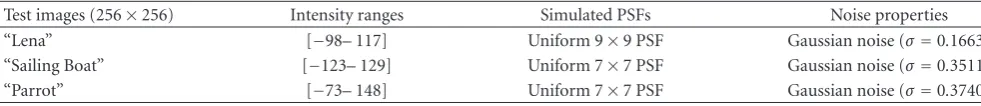
Table1: Image and degradation information for the three test images.

Test images (256×256) Intensity ranges Simulated PSFs Noise properties

“Lena” [−98– 117] Uniform 9×9 PSF Gaussian noise (σ=0.1663)

“Sailing Boat” [−123– 129] Uniform 7×7 PSF Gaussian noise (σ=0.3511)

“Parrot” [−73– 148] Uniform 7×7 PSF Gaussian noise (σ=0.3740)

Table2: Optimal parameter settings.

Test images TV prior Huber prior SA prior

“Lena” β=0.0038 β=0.026,γ=0.35 β=0.015,δ=900

“Sailing Boat” β=0.006 β=0.044,γ=0.45 β=0.015,δ=800

“Parrot” β=0.0085 β=0.025,γ=0.55 β=0.02,δ=350

results are the SNR and the improvement in signal-to-noise ratio (ISNR). ISNR is defined as

ISNR=10 log₁₀

⎛ ⎜ ⎝

M j

fj−gj

2

M j

fj−fj

2 ⎞ ⎟

⎠. (17)

HereM, f, f, andgdenote the total pixel number, the orig-inal image, the restored image, and the observed degraded image, respectively.

Restoration experiments with three 256×256 images (“Lena” (Figure 2(a)), “Sailing Boat” (Figure 3(a)), and “Par-rot” (Figure 4(a)) are performed. Image and degradation information is listed in Table 1. The three PSFs used in experiment are all normalized to 1. Observed degraded images (resp., in Figures2(b),3(b), and4(b)) were simulated by (1) using corresponding PSFs and white Gaussian noise. All of the restorations using the three images are shown in Figures2,3, and4, respectively.

4.1. Results from Diﬀerent Restoration Methods. In order to compare the proposed approaches with previous ones, we implement Wiener filter restoration, Bayesian restoration using TV prior, and Huber prior. We perform the classical Wiener filter in the DFT domain using the degraded image to estimate the image power spectrum and assuming that the additive noise variance is known. The resulting images are, respectively, shown in Figures2(c),3(c), and4(c).

The hyperparameter β for all Bayesian restorations, threshold parameter γ for Huber prior, and threshold parameter δ for the nonlocal prior are chosen manually using the SNR criteria. The used parameters for diﬀerent restorations are listed inTable 2.

The TWIST [7] and Newton-Raphson algorithm are used in restorations using TV prior and Huber prior, respectively. Restored images from above Wiener filter method are used as the initial images. The iteration number is set to be 500. The corresponding restored images from TV prior restoration are, respectively, shown in Figures 2(d), 3(d), and 4(d). And the corresponding restored images from Huber prior restoration are, respectively, shown in Figures2(e),3(e), and

4(e).

Table 3: Signal-to-noise ratio (SNR) of the observed degraded images and the restored images.

Test images Degraded

image

Wiener filter

TV prior

Huber

prior SA prior

“Lena” 6.65 15.06 15.54 15.59 15.86

“Sailing Boat” 6.97 15.76 16.43 16.45 16.91

“parrot” 7.98 16.75 17.25 17.22 17.86

Table 4: Improvement in signal-to-noise ratio (ISNR) of the observed degraded images and the restored images.

Test Images Wiener filter TV prior Huber Prior SA prior

“Lena” 5.79 8.48 8.76 9.15

“Sailing Boat” 7.12 10.10 10.54 11.13

“Parrot” 8.06 11.45 11.99 12.40

For Bayesian restoration using the proposed SA prior, the 7×7 neighborhoodNand the 7×7 comparing neighborhood

n are used. We apply above two-step Newton-Raphson algorithm with a prefixed iteration number Γ. Restored images from the fifth TV iteration are chosen as the initial images to achieve faster convergence. The total iteration number is set to be 500 withΓ=200. And the corresponding restored images are, respectively, shown in Figures2(f),3(f), and4(f).

Through comparison, we find that all of the three Bayesian restorations can effectively overcome the annoying ring effects in Wiener filter restoration. Especially, the block artifacts, which can be observed in the Bayesian approach using Huber prior and TV prior, are effectively suppressed using the proposed method. Restorations using the proposed SA prior perform better in both noise suppressing and edge preserving. Using the proposed approach, continuous regions and details are better restored with much less block artifacts produced. We can also see in Tables3and4that the proposed SA prior restoration approaches can restore images with higher SNR and ISNR values.

(7)

(a) (b) (c)

(d) (e) (f)

Figure2: (a) Original “Lena” image. (b) Degraded “Lena” image (SNR=6.65) with 9×9 uniform blur and additive white Gaussian noise (local variance=0.1663). (c) Wiener filter restoration. (d) TV prior Bayesian restoration. (e) Nonquadratic Huber prior Bayesian restoration. (f) The proposed SA prior Bayesian restoration.

Table5: Combinations of neighborhoodsN andnwith diﬀerent sizes.

a,N3×3n1×1 b,N3×3n3×3 c,N3×3n7×7

d,N7×7n1×1 e,N7×7n3×3 f,N7×7n7×7

g,N11×11n1×1 h,N11×11n3×3 i,N11×11n7×7

Table6: SNR for the restorations using the proposed SA prior with the corresponding neighborhood combinations inTable 5.

a, N3×3n1×1: 15.55 b,N3×3n3×3: 15.68 c,N3×3n7×7: 15.60

d,N7×7n1×1: 15.53 e,N7×7n3×3: 15.72 f,N7×7n7×7: 15.86

g,N11×11n1×1: 15.43 h,N11×11n3×3: 15.69 i,N11×11n7×7: 15.89

in restoration, we perform restorations of 256×256 image “Lena” using the proposed SA prior with neighborhoodsN

andnof diﬀerent sizes. The total iteration number is set to be 500 withΓ=200. Same restoration environment as above is used. The combinations of neighborhoodsN andnwith diﬀerent sizes are illustrated inTable 5.

Considering the fact that the numbers of pixels are diﬀerent for diﬀerent comparing neighborhoods n(49 for 7×7 neighborhoodn, 9 for 3×3 neighborhoodn, and 1 for 1×1 neighborhoodn), parameterδshould also change

with restorations using diﬀerent comparing neighborhoods

n. The values of parameterδfor 7×7n, 3×3n, and 1×1nare set to be 900, 400, and 125, respectively. The hyperparameter

βfor the SA prior is chosen by hand under the same strategy in terms of the SNR criteria.

We can see inTable 6that higher SNR can be obtained for largerNandn. When choosing 1×1nwithNof diﬀerent sizes, the comparing neighborhoodsn become one single-pixel and only single single-pixel intensities are compared in (11). In this situation the SA prior becomes a modified version of local Huber prior. Choosing 7×7N with 7×7n, we can restore the images with almost the same SNR as those with larger N. N and n of a suitable size (7×7 for both in this situation) might be large enough to achieve good restorations.

We also list in Table 7 the CPU time costs for above restorations using the proposed prior with above diﬀerent combinations of neighborhoods. The methods for computa-tion reduccomputa-tion inSection 3are used. As predicted, more CPU time costs are needed for the restorations using the proposed prior with largerNandn.

4.3. Iteration Monotonicity. We know from the analysis in

Section 3 that the Hessian matrix of the ψβ(f | g) in

(8)

(a) (b) (c)

(d) (e) (f)

Figure3: (a) Original “Sailing Boat” image. (b) Degraded “Sailing Boat” image (SNR=6.97) with 7×7 uniform blur and additive white Gaussian noise (local variance=0.3511). (c) Wiener filter restoration. (d) TV prior Bayesian restoration. (e) Nonquadratic Huber prior Bayesian restoration. (f) The proposed SA prior Bayesian restoration.

Table7: CPU times in terms of seconds needed for above restorations using the proposed SA prior with the corresponding neighborhood combinations inTable 5.

a,N3×3n1×1: 58.16 sec b,N3×3n3×3: 96.84 sec c,N3×3n7×7: 150.72 sec

d,N7×7n1×1: 73.72 sec e,N7×7n3×3: 118.30 sec f,N7×7n7×7: 224.60 sec

g,N11×11n1×1: 97.62 sec h,N11×11n3×3: 148.78 sec i,N11×11n7×7: 321.48 sec

of all wb j are fixed. However, before preset Γ iterations,

no strict convergence is guaranteed because the posterior energy function changes with the weighting factors which are needed to be updated in each iteration. Here, inFigure 5, we calculate and plot the posterior function energyψβ(f |

g) with respect to iteration numbers for above restoration experiment with “Lena” image. The total iteration number is set to be 1000 withΓ = 200 to include a long iteration process. We can see that the calculated posterior function energy decreases monotonically during the whole iteration process.

We thus conclude that, using the proposed algorithm, monotonic decrement of the posterior function energy can be achieved after Γ iterations when the weighting factors begin to be fixed and fixed posterior energy function is guaranteed.

5. Conclusions and Future Work Plan

(9)

(a) (b) (c)

(d) (e) (f)

Figure4: (a) Original “Parrot” image. (b) Degraded “Parrot” image (SNR=7.98) with 7×7 uniform blur and additive white Gaussian noise (local variance=0.3740). (c) Optimal Wiener filter restoration. (d) TV prior Bayesian restoration. (e) Nonquadratic Huber prior Bayesian restoration. (f) The proposed SA prior Bayesian restoration.

0 100 200 300 400 500 600 700 800 900 1000 Iteration number

P

o

st

er

ior

energ

y

0 1 2 3 4 5

×104

Figure5: Using the proposed restoration algorithm inSection 3, the calculated posterior function energy with respect to iteration number is shown.

Nevertheless, although several computation reduction approaches have been applied, the proposed approach still needs computations over large neighborhoods and estima-tions of hand-adjusted parameters (threshold δ and the sizes for neighborhoods N and n), which make it high

computational cost compared to other methods. However, considering the ever-increasing computing power and the need for high-quality restoration, the increased computation cost should not be overblamed.

Further work includes further exploring of more eﬀective guideline in determining the sizes for neighborhoodsNand

n under diﬀerent noise levels and estimation of threshold parameter δ and in finding eﬀective ways to lower the computation cost.

Acknowledgment

This research was supported by National Basic Research Program of China under Grant no. 2010CB732503.

References

[1] A. Srivastava, A. B. Lee, E. P. Simoncelli, and S. -C. Zhu, “On advances in statistical modeling of natural images,”Journal of Mathematical Imaging and Vision, vol. 18, no. 1, pp. 17–33, 2003.

(10)

[3] R. Molina, “On the hierarchical Bayesian approach to image restoration: applications to astronomical images,”IEEE Trans-actions on Pattern Analysis and Machine Intelligence, vol. 16, no. 11, pp. 1122–1128, 1994.

[4] G. Archer and D. M. Titterington, “On some Bayesian/ regularization methods for image restoration,”IEEE Transac-tions on Image Processing, vol. 4, no. 7, pp. 989–995, 1995. [5] S. Geman and D. Geman, “Stochastic relaxation, Gibbs

distributions, and the bayesian restoration of images,”IEEE Transactions on Pattern Analysis and Machine Intelligence, vol. 6, no. 6, pp. 721–741, 1984.

[6] N. P. Galatsanos and A. K. Katsaggelos, “Methods for choosing the regularization parameter and estimating the noise variance in image restoration and their relation,”IEEE Transactions on Image Processing, vol. 1, no. 3, pp. 322–336, 1992.

[7] J. M. Bioucas-Dias and M. A. T. Figueiredo, “A new TwIST: two-step iterative shrinkage/thresholding algorithms for image restoration,”IEEE Transactions on Image Processing, vol. 16, no. 12, pp. 2992–3004, 2007.

[8] Y. Wan and R. Nowak, “A Bayesian multiscale approach to joint image restoration and edge detection,” in Wavelet Applications in Signal and Image Processing VII, vol. 3813 of

Proceedings of SPIE, pp. 73–84, Denver, Colo, USA, July 1999. [9] M. A. T. Figueiredo and R. D. Nowak, “An EM algorthim for

wavelet-besed image restoration,”IEEE Transactions on Image Processing, vol. 12, no. 8, pp. 906–916, 2003.

[10] J. M. Bioucas-Dias, “Bayesian wavelet-based image deconvo-lution: a GEM algorithm exploiting a class of heavy-tailed priors,”IEEE Transactions on Image Processing, vol. 15, no. 4, pp. 937–951, 2006.

[11] R. Neelamani, H. Choi, and R. Baraniuk, “ForWaRD: Fourier-wavelet regularized deconvolution for Ill-conditioned sys-tems,”IEEE Transactions on Signal Processing, vol. 52, no. 2, pp. 418–433, 2004.

[12] C. A. Bouman and K. Sauer, “A generalized Gaussian image

model for edge-preserving MAP estimation,” IEEE

Transac-tions on Image Processing, vol. 2, no. 3, pp. 296–310, 1993. [13] Y. Wang, J. Liu, and X. Tang, “Robust 3D face recognition

by local shape diﬀerence boosting,” to appear in IEEE

Transactions on Pattern Analysis and Machine Intelligence. [14] L. I. Rudin, S. Osher, and E. Fatemi, “Nonlinear total variation

based noise removal algorithms,”Physica D, vol. 60, no. 1–4, pp. 259–268, 1992.

[15] A. Chambolle, “An algorithm for total variation minimization and applications,”Journal of Mathematical Imaging and Vision, vol. 20, no. 1-2, pp. 89–97, 2004.

[16] M. Mignotte, “A segmentation-based regularization term for image deconvolution,”IEEE Transactions on Image Processing, vol. 15, no. 7, pp. 1973–1984, 2006.

[17] G. K. Chantas, N. P. Galatsanos, and A. C. Likas, “Bayesian restoration using a new nonstationary edge-preserving image prior,”IEEE Transactions on Image Processing, vol. 15, no. 10, pp. 2987–2997, 2006.

[18] G. Chantas, N. Galatsanos, and A. Likas, “Bayesian image restoration based on variational inference and a product of student-t priors,” in Proceedings of the 17th IEEE Interna-tional Workshop on Machine Learning for Signal Processing (MLSP ’07), pp. 93–98, Thessaloniki, Greece, August 2007. [19] Y. Chen, J. Ma, Q. Feng, L. Luo, P. Shi, and W. Chen,

“Non-local prior Bayesian tomographic reconstruction,”Journal of Mathematical Imaging and Vision, vol. 30, no. 2, pp. 133–146, 2008.

[20] Y. Chen, D. Z. Gao, C. Nie, et al., “Bayesian statistical reconstruction for low-dose X-ray computed tomography

using an adaptive-weighting nonlocal prior,” Computerized

Medical Imaging and Graphics, vol. 33, no. 7, pp. 495–500, 2009.

[21] Y. Chen, L. Hao, X. Ye, W. Chen, L. Luo, and X. Yin, “PET transmission tomography using a novel nonlocal MRF prior,”

Computerized Medical Imaging and Graphics, vol. 33, no. 8, pp. 623–633, 2009.

[22] J. W. Woods, S. Dravida, and R. Mediavilla, “Image estimation using doubly stochastic Gaussian random field models,”IEEE Transactions on Pattern Analysis and Machine Intelligence, vol. 9, no. 2, pp. 245–253, 1987.

[23] D. F. Yu and J. A. Fessler, “Edge-preserving tomographic reconstruction with nonlocal regularization,”IEEE Transac-tions on Medical Imaging, vol. 21, no. 2, pp. 159–173, 2002. [24] A. Buades, B. Coll, and J.-M. Morel, “A non-local algorithm

for image denoising,” in Proceedings of the IEEE Computer

Society Conference on Computer Vision and Pattern Recognition (CVPR ’05), vol. 2, pp. 60–65, San Diego, Calif, USA, June 2005.

[25] C. A. Bouman and K. Sauer, “A unified approach to statistical

tomography using coordinate descent optimization,” IEEE

Transactions on Image Processing, vol. 5, no. 3, pp. 480–492, 1996.

[26] S. Sotthivirat and J. A. Fessler, “Image recovery using

partitioned-separable paraboloidal surrogate coordinate

ascent algorithms,”IEEE Transactions on Image Processing, vol. 11, no. 3, pp. 306–317, 2002.

[27] K. Lange, “Convergence of EM image reconstruction algo-rithms with Gibbs smoothing,”IEEE Transactions on Medical Imaging, vol. 9, no. 4, pp. 439–446, 1990.