Volume 2010, Article ID 879874,10pages doi:10.1155/2010/879874
Research Article
Robust Time-Frequency Distributions with
Complex-Lag Argument
Nikola ˇ
Zari´c, Irena Orovi´c, and Srdjan Stankovi´c
Faculty of Electrical Engineering, University of Montenegro, Podgorica 20000, Montenegro
Correspondence should be addressed to Nikola ˇZari´c,[email protected]
Received 30 December 2009; Accepted 1 March 2010
Academic Editor: Igor Djurovi´c
Copyright © 2010 Nikola ˇZari´c et al. This is an open access article distributed under the Creative Commons Attribution License, which permits unrestricted use, distribution, and reproduction in any medium, provided the original work is properly cited.
The robust time-frequency distributions with complex-lag argument are proposed. They can provide an accurate estimation of fast varying instantaneous frequency in the presence of noise with heavy-tailed probability density function. The L-estimate form of this distribution is defined and it includes the L-estimate form of Wigner distribution as a special case. A modification for multicomponent signal representation is proposed, as well. Theoretical considerations are illustrated by the examples.
1. Introduction
Nonstationary signals such as speech, radar, seismic, sonar, and biomedical signals can be found in many practical applications. Due to time-varying spectra of these signals, time-frequency analysis has been used in their analysis. For different types of signals, various time-frequency distribu-tions (TFDs) have been proposed [1–5].
In real applications we deal with signals corrupted by noise. If noise is additive with Gaussian probability density function (pdf), the standard time-frequency distributions represent a maximum likelihood (ML) estimate [6]. How-ever, if the signal is corrupted by noise with heavy-tailed pdf (usually caused by environmental or human-made activi-ties), the standard TFDs produce poor results. Consequently, the robust time-frequency distributions have been intro-duced [6–12]. The simplest and the most commonly used robust time-frequency representation is the robust short-time Fourier transform (STFT). The marginal median robust STFT has been introduced as an ML estimate of signals with Laplacian noise [8]. This form can also be successfully used for other types of heavy-tailed noises. The L-estimate robust STFT is introduced for signals with a mixture of Gaussian and impulse noises [9]. As in the case of the standard STFT, the main drawback of the robust STFT is a poor frequency resolution. In order to improve the time-frequency concentration, the robust forms of the Wigner
distribution (WD) have been introduced [9–12]. They can provide an ideal concentration for signals with a linear instantaneous frequency (IF). However, for multicomponent signals the cross-terms appear. The robust S-method that combines good properties of the STFT and the WD has been introduced to provide a cross-terms free representation [12]. However, it cannot provide good concentration for signals with fast varying IF. Thus, the time-frequency distributions with complex-lag argument have been used to estimate nonlinear and fast IF variations [13–20]. Similarly as other TFDs, these distributions provide poor signal representation in the presence of heavy-tailed noise.
In this paper we propose a robust form of the N th-order complex-lag time-frequency distribution (CTD). An arbitrary high concentration can be achieved by increasing the distribution orderN. The standard CTD has been defined as convolution of the WD and the Fourier transform of the higher order complex-lag moment, called concentration function (CF) [17, 18]. Similarly, the robust CTD can be obtained as convolution of the robust WD and CF forms. Additionally, a cross-terms free robust complex-lag time-frequency distribution is proposed for multicomponent signals.
proposed inSection 3. The advantages of the proposed dis-tributions are proven through various examples inSection 4. Concluding remarks are given inSection 5.
2. Theoretical Background
2.1. Robust Short-Time Fourier Transform. Consider the noisy signalx(n) = s(n) +v(n), wheres(n) is a complex-valued signal corrupted with complex-complex-valued noise v(n). The STFT can be obtained as a solution of the following optimization problem:
STFT(n,k)=arg min
μ Ns/2−1
m=−Ns/2
F(e(n,k,m)), (1)
whereF(e) is the loss function, whilee(n,k,m) is the error function:
e(n,k,m)=x(n+m)e−j2πmk/Ns−μ. (2)
The number of samples within the window is denoted asNs, whileμrepresents complex-valued optimization parameter. In the case of the loss function F(e) = |e|2
, the standard STFT is obtained:
STFTS(n,k)
=N1
s Ns/2−1
m=−Ns/2
x(n+m)e−j2πmk/Ns
=mean
x(n+m)e−j2πmk/Ns,m∈
−Ns
2 , Ns 2 . (3)
The quadratic loss function is the ML estimate of a signal corrupted with Gaussian noise. Hence, the standard STFT is applicable in this case. Nevertheless, when impulse noise is present, the quadratic loss function yields poor results. Therefore, other loss functions should be used. For instance, it has been shown that the loss functionF(e)= |e|exhibits a robust behavior for heavy-tailed noise (e.g., Cauchy noise, Laplacian noise) [6, 11, 21]. The implicit solution of the optimization problem in (1) for F(e) = |e| requires a computationally demanding iterative procedure. In order to avoid such an iterative procedure, the marginal median estimate, with the loss functionF(e) = |Re(e)|+|Im(e)|, has been introduced in [8]:
STFTM(n,k)
=median
Rex(n+m)e−j2πmk/Ns,m∈
−Ns
2 ,
Ns
2
+j·median
Imx(n+m)e−j2πmk/Ns,m∈
−Ns
2 , Ns 2 . (4)
If the signal is corrupted by a mixture of Gaussian and impulse noise, the L-estimate robust STFT is used. It is defined as [9]
STFTL(n,k)=
Ns/2−1
i=−Ns/2
ai ri(n,k) +j·ii(n,k),
ri(n,k)∈R(n,k),
R(n,k)=
Rex(n+m)e−j2πmk/Ns,m∈
−Ns
2,
Ns
2
ii(n,k)∈I(n,k),
I(n,k)=
Imx(n+m)e−j2πmk/Ns,m∈
−Ns
2 , Ns 2 , (5)
where the elementsri(n,k) andii(n,k) are sorted in nonde-creasing order asri(n,k)≤ri+1(n,k) andii(n,k)≤ii+1(n,k), respectively. The coefficientsaiare given as
ai= ⎧ ⎪ ⎨ ⎪ ⎩ 1
Ns(1−2α)+4α, fori∈[(Ns−2)α,α(2−Ns)+Ns−1],
0, elsewhere,
(6)
whereNsis even, while the parameterαtakes values within the range [0, 1/2].Forα=0 andα=1/2 the standard STFT and the marginal median STFT are obtained, respectively. Higher value ofαprovides an enhanced reduction of heavy-tailed noise, while smaller value of α improves spectral characteristics. Thus, depending on the application, the value of parameterαshould be chosen to provide good trade-off between these requirements.
The robust spectrogram is obtained as
SPECh(n,k)=Re{STFTh(n,k)}2
+ Im{STFTh(n,k)}2 ,
(7)
where STFThmay be STFTMor STFTL.
2.2. Robust Quadratic Time-Frequency Distributions. The previous concept has been extended to the Wigner distribu-tion. The WD can be obtained as a solution of the following optimization problem:
WD(n,k)=arg min
μ Ns/2−1
m=−Ns/2
F(e(n,k,m)),
e(n,k,m)=Rex(n+m)x(n−m)e−j4πmk/Ns−μ, (8)
where x denotes the complex conjugate of x. For the loss functionF(e)= |e|2, the standard WD follows:
WDS(n,k)=meanRex(n+m)x(n−m)e−j4πmk/Ns,
m∈
−Ns
The median-based robust WD has been defined in [8] as a solution of optimization problem in (8), for the loss function
F(e)= |e|:
WDM(n,k)=medianRex(n+m)x(n−m)e−j4πkm/Ns,
m∈
−Ns
2 ,
Ns
2
.
(10)
The L-estimate robust WD can be written as [9]
WDL(n,k)=
Ns/2−1
i=−Ns/2
airi(n,k),
ri(n,k)∈R(n,k)=
Rex(n+m)x(n−m)e−j4πmk/Ns,
m∈
−Ns
2,
Ns
2
,
(11)
where the elementsri(n,k) are sorted in nondecreasing order asri(n,k)≤ri+1(n,k), while the coefficientsaiare defined by (6). The marginal median WD follows forα=1/2.
The WD can be calculated by using STFT:
RWDh(n,k)=Ns/
2−1
l=−Ns/2
STFTh(n,k+l)STFTh(n,k−l),
(12)
where STFTh can be the median-based STFT or the L-estimate STFT.
The robust S-method has been introduced in order to reduce or remove cross-terms in the robust WD. It can be written in the following form [12]:
RSMh(n,k)= L
l=−L
P(l)STFTh(n,k+l)STFTh(n,k−l),
(13)
where P(l) is a frequency domain window with its width equal to 2L+ 1. For L = 0 and L = Ns/2 the robust
spectrogram and the robust WD are obtained, respectively. More details about parameterLselection can be found in [5].
3. Robust Complex-Lag Time-Frequency
Distributions
The time-frequency distributions with complex-lag argu-ment have been introduced for signals with fast varying instantaneous frequency. The general form of the standard
Nth-order complex-lag time-frequency distribution can be written as [18]
CTDN(n,k)=
Ns/2−1
m=−Ns/2
x(n+m)x(n−m)c(n,m)e−j(2π/Ns)Nmk
=
Ns/2−1
l=−Ns/2
WD(n,k+l)CF(n,k−l),
(14)
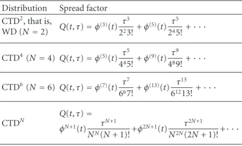
Table1: Spread factors for some time-frequency distributions. Distribution Spread factor
CTD2, that is,
WD (N=2) Q(t,τ)=φ(3)(t) τ3
223!+φ (5)(t) τ5
245!+· · ·
CTD4(N=4) Q(t,τ)=φ(5)(t) τ5
445!+φ(9)(t)
τ9
489!+· · ·
CTD6(N=6) Q(t,τ)=φ(7)(t) τ7
667!+φ
(13)(t) τ13
61213!+· · ·
CTDN Q
(t,τ)=
φN+1(t) τN+1
NN(N+ 1)!+φ2N+1(t)
τ2N+1
N2N(2N+ 1)!+· · ·
where the standard WD is given by (9), whileCF(n,k) is the Fourier transform of the complex-lag signal moment:
c(n,m)=N/
2−1
p=1
xwN,pn+wN ,pm
x−wN,pn−wN ,pm
, (15)
where N is an even number, representing the distribution order, while the quantitywN,p=ej2π p/N, p=1,. . .,N/2−1
defines the equidistant roots on the unit circle. It has been shown [17–19] that the distribution defined by (14) can provide an arbitrarily high concentration by increasing N. Namely, the complex-lag distributions significantly reduce the spread factor produced by higher phase derivatives. For example, the fourth-order distribution:
CTD4(n,k)
= Ns/
2−1
m=−Ns/2
x(n+m)x(n−m)x−j n+jm
×xj n−jme−j(2π/Ns)4mk
(16)
contains the number of spread terms that is twice smaller than for the WD (Table 1). Furthermore, the sixth-order distribution is obtained for the roots {w1,w2} = {1/2 +
j√3/2, −1/2 +j√3/2}:
CTD6(n,k)
=
Ns/2
m=−Ns/2
s(n+m)s−1(n−m)× s(n+w1m)s−1(n−w1m)
w∗
1
× s(n+w2m)s−1(n−w2m)
w∗
2e−j(2π/Ns)6mk,
(17)
In order to obtainc(n,m), the signal with complex-lag argumentx(n±wN,pm) is calculated by using the concept
of analytic extension as follows:
xn±wN,pm
=
Ns/2−1
k=−Ns/2
XS(k)ej(2π/Ns)(n±wN,pm)k
=
Ns/2−1
k=−Ns/2
XS(k)e∓(2π/Ns)wiN,pmkej(2π/Ns)(n±wrN,pm)k, (18)
where wrN,p = Re{wN,p},wiN,p = Im{wN,p}, whileXS(k)
is the standard Fourier transform. The coordinate m is multiplied bywrN,p. The influence of this term can be such
that an additional oversampling (or interpolations) of signal
x(n) is required.
By analogy with the standard CTD, the robust CTD can be defined as
RCTDN(n,k)=
Ns/2−1
l=−Ns/2
RWD(n,k+l)RCF(n,k−l), (19)
where RWD is the robust WD, while robust CF (RCF) is obtained as a solution of the optimization problem:
CF(n,k)=arg min
μ Ns/2−1
m=−Ns/2
F(e(n,k,m)),
e(n,k,m)=c(n,m)e−j(2π/Ns)Nmk−μ,
(20)
for the loss functionF(e)= |e|.The robust WD calculation has been already presented, while the robust CF can be obtained as a solution of nonlinear equation:
RCF(n,k)
=Ns/2−1 1
m=−Ns/2(1/|e(n,k,m)|)
×
Ns/2−1
m=−Ns/2 1
|e(n,k,m)|c(n,m)e−j(2π/Ns)Nmk,
e(n,k,m)=c(n,m)e−j(2π/Ns)Nmk−RCF(n,k).
(21)
The iterative procedure for the nonlinear equation (21) is even more demanding than in the cases of robust STFT and robust WD calculations [6, 11]. Namely, to calculate
c(n,m), the robust form of (18) has to be used. It requires an additional iterative procedure. Hence, the CF calculation requires nested iterative procedures, inappropriate for prac-tical realization.
3.1. L-Estimate Form of the Robust CTD. The marginal median and the L-estimate approach can be used to over-come disadvantages of iterative procedure for the robust CTD calculation. In the sequel, only the L-estimate approach is considered, since the marginal median follows as a special
case of the L-estimate forms forα=1/2. Also, the L-estimates exhibit enhanced performance in the presence of mixture of Gaussian and impulse noise, common to real applications. Thus, the L-estimate approach is used to define the robust CTD.
Having in mind (19), the L-estimate robust CTD can be obtained as a convolution of the L-estimate robust WD and the L-estimate robust CF. By analogy with the robust WD, the L-estimate approach is used for the robust CF calculation, as follows:
RCFL(n,k)=
Ns/2−1
i=−Ns/2
ai cri(n,m) +j·cii(n,m), (22)
wherecri(n,k) andcii(n,k) are the elements of
R(n,k)=Re
rc(n,m)e−j(2π/Ns)Nmk,m∈−Ns
2 ,
Ns
2
,
I(n,k)=Im
rc(n,m)e−j(2π/Ns)Nmk,m∈−Ns
2 ,
Ns
2
,
(23)
respectively. They are sorted in nondecreasing order:
cri(n,k) ≤ cri+1(n,k) and cii(n,k) ≤ cii+1(n,k). The coefficientsai are given by (6), whilerc(n,m) represent the robust complex-lag signal moment:
rc(n,m)=N/
2−1
p=1
crp(n,m)cip(n,m),
crp(n,m)=ejwrN,pangle(x(n+wN,pm)/x(n−wN,pm)),
cip(n,m)=ejwiN,plog|x(n−wN,pm)/x(n+wN,pm)|.
(24)
The numerical realization is simplified by using the angle and log|·|functions. Namely, for a signal in the formx(t)=
Aejφ(t), the amplitude modulation terms that may appear in the calculation ofcrp(n,m) andcip(n,m) are eliminated, [18]. Also, calculation of signal raised to powerjis avoided by using the exponential with log| · |function, [14]. The signal with the complex-lag argument is obtained as
xL
n±wN,pm
=
Ns/2−1
k=−Ns/2
XL(k)ej2π(n±wN,pm)k, (25)
whereXL(k) represents the L-estimate of Fourier transform:
XL(k)= Ns/2−1
i=−Ns/2
ai ri(k) +j·ii(k), (26)
whereri(k)∈R(k),R(k)= {Re(x(n)e−j2πkn/Ns),n∈[0,Ns− 1)} and ii(k) ∈ I(k), I(k) = {Im(x(n)e−j2πnk/Ns),n ∈ [0,Ns−1)}are such thatri(k)≤ri+1(k) andii(k)≤ii+1(k).
Finally, the L-estimate of complex-lag time-frequency distribution is:
120 100 80 60 40 20
20 40 60 80 100 120
(a)
120 100 80 60 40 20
20 40 60 80 100 120
(b)
120 100 80 60 40 20
20 40 60 80 100 120
(c)
120 100 80 60 40 20
20 40 60 80 100 120
(d)
120 100 80 60 40 20
20 40 60 80 100 120
(e)
Figure1: Time-frequency representations for signalx1(n) by using (a) the standard WD, (b) the L-estimate WD, (c) the standard CTDN=4,
3.2. Robust CTD Form for Multicomponent Signals. Note that the robust CTD form (defined by (27)) can be used for monocomponent signals. However, in the case of multicom-ponent signal: x(n) = Qq=1sq(n) +v(n), the cross-terms appear. Thus, it is necessary to modify (27). The robust S-method, as a cross-terms free distribution, will be used instead of the robust WD, while a modification providing a cross-terms free robust CF should be introduced. In that sense, the signal with complex-lag argument is separately calculated for each component. The component separation is performed by using the robust STFT. Namely, theqth signal component is obtained as
xL
n±wN,pm
q
=
Wq
k=−Wq
STFTLn,k+kq(n)ej(k+kq(n))(n±wN,pm), (28)
wherekq(n)=arg{maxkSTFTL(n,k)}is the position of the
qth signal component maximum in the L-estimate robust STFT. It is assumed that the q-th signal component is of 2Wq+1 width; that is, it is within the region [kq(n)-Wq,
kq(n)+Wq]. Observe that the cross-terms will be avoided, if the distance between signal components is higher than 2Wq(see [14] for details). After the first signal component is obtained, the values of STFTL(n,k) within the region [kq(n
)-Wq, kq(n)+Wq] will be set to 0. Then, this procedure is repeated for other components.
Furthermore, for theqth signal component the complex-lag signal momentscr(n,m)qandci(n,m)qare
cr(n,m)q
=
N/2−1
p=1
crp(n,m)q= N/2−1
p=1
ejwrN,pangle(xL(n+wN,pm)q/xL(n−wN,pm)q) ,
ci(n,m)q
=
N/2−1
p=1
cip(n,m)q=
N/2−1
p=1
ejwiN,plog|xL(n−wN,pm)q/xL(n+wN,pm)q|.
(29)
For all signal components we havecr(n,m)=qQ=1cr(n,m)q and ci(n,m) = qQ=1ci(n,m)q. By using the L-estimate
approach, two corresponding robust CFs can be defined as
RCFrL(n,k)=
Ns/2−1
i=−Ns/2
ai vri(n,m) +jvii(n,m),
RCFiL(n,k)=
Ns/2−1
i=−Ns/2
ai uri(n,m) +juii(n,m),
(30) 0 10 20 30 40 50 60 Standard WD L-estimate robust WD Standard CTD
Median CTD L-estimate RCTD
Figure 2: MSE of instantaneous frequency estimation in the presence of heavy-tailed noise.
wherevri(n,k) andvii(n,k) (sorted in nondescending order) are elements of:
Rv(n,k)=Re
cr(n,m)e−j(2π/Ns)Nmk,m∈−Ns
2 ,
Ns
2
,
Iv(n,k)=Im
cr(n,m)e−j(2π/Ns)Nmk,m∈
−Ns
2 , Ns 2 , (31)
respectively. Similarly,uri(n,k) anduii(n,k) are elements of:
Ru(n,k)=Re
ci(n,m)e−j(2π/Ns)Nmk,m∈
−Ns
2 ,
Ns
2
,
Iu(n,k)=Im
ci(n,m)e−j(2π/Ns)Nmk,m∈
−Ns
2 , Ns 2 , (32)
whereuri(n,k)≤uri+1(n,k) anduii(n,k)≤uii+1(n,k). The cross-terms free robust CF is:
RCFL(n,k)=
L
l=−L
P(l)CFrL(n,k+l)CFiL(n,k−l). (33)
Finally, the L-estimate robust CTD for multicomponent signals can be written in the form:
RCTDNL(n,k)=
L
l=−L
P(l)SML(n,k+l)RCFL(n,k−l).
(34)
120 100 80 60 40 20
20 40 60 80 100 120
(a)
120 100 80 60 40 20
20 40 60 80 100 120
(b)
120 100 80 60 40 20
20 40 60 80 100 120
(c)
Figure3: Time-frequency representations for signaly(n) by using: (a) the L-estimate WD, (b) the L-estimate RCTDN=4, and (c) the
L-estimate RCTDN=6.
4. Examples
Highly nonstationary signals with fast varying instantaneous frequencies are considered. The signals are corrupted with heavy-tailed noise. The standard and the robust forms of CTD are considered and compared with corresponding forms of the Wigner distribution.
Example 1. Consider a noisy signal:
x(n)=e2j(6 cos(πn)+2/3 cos(3πn)+2/3 cos(5πn))+ξ(n), (35) where ξ(n) is heavy-tailed complex valued noise (cube of Gaussian noise):
ξ(n)=0.5ξ13(n) + 0.5jξ23(n), (36) where ξ1(n) andξ2(n) are mutually independent Gaussian noises (zero mean with variance equal to 1). The time intervalt∈[−2, 2], with sampling rateT =1/128, is used. The Gaussian window of Ns = 128 width is applied in all cases.
The L-estimate forms are calculated by using param-eter α = 3/8 for all distributions. Namely, this value provides satisfying trade-off between noise reduction and distribution concentration. For a given signal, the stan-dard WD, the L-estimate WD, the stanstan-dard CTDN=4, the marginal median RCTDN=4 (obtained according to (27) with α=1/2), and the L-estimate RCTDN=4 are shown in
120 100 80 60 40 20
20 40 60 80 100 120
(a)
120 100 80 60 40 20
20 40 60 80 100 120
(b)
120 100 80 60 40 20
20 40 60 80 100 120
(c)
120 100 80 60 40 20
20 40 60 80 100 120
(d)
Figure4: Time-frequency representation for multicomponent signalx(n) by using (a) the standard SM, (b) the L-estimate SM, (c) the standard CTDN=4, and (d) the L-estimate RCTDN=4.
The mean squared error (MSE) is used as a quantitative measure of performance, for all distributions:
MSE=N1
s Ns
n=1
ϕ(n)−ϕ(n)2
, (37)
where ϕ(n) is the true IF, while ϕ(n) is the estimated IF:
ϕ(n)=arg{maxkSTFT(n,k)}. The mean values of MSEs are given inFigure 2for 100 realizationsof noises. Note that the L-estimate RCTDN=4provides the lowest MSE.
In the presence of Gaussian noise, the performance of L-estimate RCTDN=4 is similar to the performance of the standard CTDN=4. The MSEs of IF estimation, calculated as a mean value for 100 realizations of Gaussian noises, are given inTable 2.
Example 2. This example aims to illustrate how the distri-bution order has to be increased to achieve concentration
Table2: The MSE of instantaneous frequency estimation in the presence of Gaussian noise.
Distribution MSE
Standard CTDN=4 2.45
L-estimate RCTDN=4 2.56
improvement. Namely, in the case of signal with IF variations that are faster than in the previous example, for example,
y(n)=e2j(3 cos(1.5πn)+2/3 cos(7πn)+1/2 cos(5πn))+ξ(n), (38)
Table3: The MSE of instantaneous frequency estimation.
Distribution MSE
L-estimate WD 51.83
L-estimate RCTDN=4 8.52
L-estimate RCTDN=6 3.45
As expected, the L-estimate WD is not suitable for analysis. Significant improvements were obtained with the L-estimate RCTDN=4, while the best results are achieved by using the L-estimate RCTDN=6 in this example. The MSE of instantaneous frequency estimation is given in Table 3
for 100 realizations of noises. Note that the lowest MSE is obtained for the L-estimate RCTDN=6distribution.
Example 3. Consider a noisy multicomponent signal:
z(n)=ej(6 cos((3/2)πn)−(4/3) cos(7πn)+cos(5πn)+15πn)
+ej(7,5π(0.5n4−0.8πn2−8,5πn)
+ 0.5ξ3
1(n) + 0.5jξ23(n),
(39)
whereξ1(n) andξ2(n) represent Gaussian noises. The same parameters for time interval, window, and noise strength are used as in theExample 2. The results for the standard SM, the L-estimate SM, the standard CTDN=4, and the L-estimate RCTDN=4are shown inFigure 4.
Note that both the standard SM and the standard CTDN=4 cannot provide satisfactory results due to the presence of impulse noise. The L-estimate SM provides good estimation for the component with slow varying instantaneous frequency (Figure 4(b)). However, it cannot follow the fast IF variationsfor the second signal component. The L-estimate RCTDN=4provides satisfying concentration for both components (Figure 4(d)).
5. Conclusion
The L-estimate-based robust Nth-order complex-lag time-frequency distribution has been proposed. It provides an efficient estimation for nonstationary signals corrupted with a mixture of Gaussian and heavy-tailed impulse noise. Additionally, we proposed the modified L-estimate robust CTD form that provides a cross-terms free representation for multicomponent signals.
The L-estimate and standard distribution approaches could be combined in some future work to reduce the calculation complexity. Also, the future research could be focused to generalize the proposed approach to the class of complex-time distributions based on the ambiguity domain [20].
Acknowledgment
This work is supported by the Ministry of Education and Science of Montenegro.
References
[1] L. Cohen,Time-Frequency Analysis, Prentice-Hall, Englewood Cliffs, NJ, USA, 1995.
[2] B. Boashash,Time-Frequency Analysis and Processing, Elsevier, Amsterdam, The Netherlands, 2003.
[3] B. Boashash, “Estimating and interpreting the instantaneous frequency of a signal—part 1: fundamentals,” Proceedings of the IEEE, vol. 80, no. 4, pp. 520–538, 1992.
[4] F. Hlawatsch and G. F. Boudreaux-Bartels, “Linear and quadratic time-frequency signal representations,”IEEE Signal Processing Magazine, vol. 9, no. 2, pp. 21–67, 1992.
[5] LJ. Stankovi´c, “A method for time-frequency analysis,”IEEE Transactions on Signal Processing, vol. 42, no. 1, pp. 225–229, 1994.
[6] V. Katkovnik, “Robust M-periodogram,”IEEE Transactions on Signal Processing, vol. 46, no. 11, pp. 3104–3109, 1998. [7] V. Katkovnik, I. Djurovi´c, and LJ. Stankovi´c, “Instantaneous
frequency estimation using robust spectrogram with varying window length,”AEU—International Journal of Electronics and Communications, vol. 54, no. 4, pp. 193–202, 2000.
[8] I. Djurovi, V. Katkovnik, and LJ. Stankovi´c, “Median filter based realizations of the robust time-frequency distributions,” Signal Processing, vol. 81, no. 8, pp. 1771–1776, 2001. [9] I. Djurovi´c, LJ. Stankovi´c, and J. F. B¨ohme, “Robust
L-estimation based forms of signal transforms and time-frequency representations,”IEEE Transactions on Signal Pro-cessing, vol. 51, no. 7, pp. 1753–1761, 2003.
[10] V. Katkovnik, I. Djurovi´c, and LJ. Stankovi´c, “Robust time-frequency distributions,” in Time-Frequency Signal Analysis and Applications, B. Boashash, Ed., pp. 392–399, Elsevier, Amsterdam, The Netherlands, 2003.
[11] I. Djurovi´c and LJ. Stankovi´c, “Robust wigner distribution with application to the instantaneous frequency estimation,” IEEE Transactions on Signal Processing, vol. 49, no. 12, pp. 2985–2993, 2001.
[12] I. Djurovi´c, LJ. Stankovi´c, and B. Barkat, “Robust time-frequency distributions based on the robust short time Fourier transform,”Annales des Telecommunications/Annals of Telecommunications, vol. 60, no. 5-6, pp. 681–697, 2005. [13] S. Stankovi´c and LJ. Stankovi´c, “Introducing time-frequency
distribution with a ‘complex-time’ argument,” Electronics Letters, vol. 32, no. 14, pp. 1265–1267, 1996.
[14] LJ. Stankovi´c, “Time-frequency distributions with complex argument,”IEEE Transactions on Signal Processing, vol. 50, no. 3, pp. 475–486, 2002.
[15] M. Morelande, B. Senadji, and B. Boashash, “Complex-lag polynomial Wigner-Ville distribution,” inProceedings of the 10th IEEE Annual Conference on Speech and Image Technologies for Computing and Telecommunications (TENCON ’97), vol. 1, pp. 43–46, Brisbane, Australia, December 1997.
[16] G. Viswanath and T. V. Sreenivas, “IF estimation using higher order TFRs,”Signal Processing, vol. 82, no. 2, pp. 127–132, 2002.
[17] C. Cornu, S. Stankovi´c, C. Ioana, A. Quinquis, and LJ. Stankovi´c, “Generalized representation of phase derivatives for regular signals,”IEEE Transactions on Signal Processing, vol. 55, no. 10, pp. 4831–4838, 2007.
[19] S. Stankovi´c and I. Orovic, “Effects of Cauchy integral formula discretization on the precision of IF estimation: unified approach to complex-lag distribution and its L-form,”IEEE Signal Processing Letters, vol. 16, no. 4, pp. 327–330, 2009. [20] I. Orovi´c and S. Stankovi´c, “A class of highly concentrated
time-frequency distributions based on the ambiguity domain representation and complex-lag moment,”EURASIP Journal on Advances in Signal Processing, vol. 2009, Article ID 935314, 9 pages, 2009.