Volume 2007, Article ID 30253,10pages doi:10.1155/2007/30253
Research Article
Modelling and Order of Acoustic Transfer Functions Due to
Reflections from Augmented Objects
Martin Kuster1, 2and Diemer de Vries1
1Laboratory of Acoustical Imaging and Sound Control, Department of Imaging Science and Technology,
Faculty of Applied Sciences, Delft University of Technology , 2600 Delft, GA, The Netherlands 2Sonic Arts Research Centre, Faculty of Engineering and Physical Sciences, Queen’s University Belfast,
Belfast, BT7 1NN, UK
Received 30 April 2006; Revised 29 September 2006; Accepted 14 October 2006
Recommended by Aki H¨arm¨a
It is commonly accepted that the sound reflections from real physical objects are much more complicated than what usually is and can be modelled by room acoustics modelling software. The main reason for this limitation is the level of detail inherent in the physical object in terms of its geometrical and acoustic properties. In the present paper, the complexity of the sound reflections from a corridor wall is investigated by modelling the corresponding acoustic transfer functions at several receiver positions in front of the wall. The complexity for different wall configurations has been examined and the changes have been achieved by altering its acoustic image. The results show that for a homogenous flat wall, the complexity is significant and for a wall including various smaller objects, the complexity is highly dependent on the position of the receiver with respect to the objects.
Copyright © 2007 M. Kuster and D. de Vries. This is an open access article distributed under the Creative Commons Attribution License, which permits unrestricted use, distribution, and reproduction in any medium, provided the original work is properly cited.
1. INTRODUCTION
For the simulation and prediction of the acoustics in closed spaces, the geometry and acoustic properties of the en-closing boundaries are the primary parameters. The acoustic properties are represented by the acoustic impedance of the boundary. For a simple shoebox room with perfectly rigid walls (i.e., infinite acoustic impedance), the method of mir-ror image sources leads to a solution that satisfies the wave
equation exactly [1]. In practice, rooms are neither of
sim-ple shoebox shape nor are the walls perfectly rigid. Instead, the modelling of all geometric details down to the order of the shortest acoustic wavelength would be required and the acoustic impedances of practical materials are generally
com-plex, frequency-dependent, and nonlocally reacting [2].
One of the primary aims in room acoustics research over the past two to three decades has been the realistic and reli-able prediction of room acoustics from a subset of the de-tailed geometric and acoustic information required
theo-retically [3–5]. In particular, the scattering of sound from
nonsmooth finite-size surfaces, leading to diffuse reflections
[6–9] and diffraction [10–12], has been recognised as one, if
not the, key contributing factor.
The research presented in the current paper aims to shed some light on the complexity of measured reflected sound from a single wall comprising a number of smaller objects. As an objective parameter, the complexity is measured by the required model order of the acoustic transfer function (ATF) resulting from the reflections/scattering from the wall. The interesting questions to be raised are to what extent is the complexity of the ATF dependent on the structural details of the wall in the immediate vicinity of (i) the receiver in the case of scattering and/or (ii) the specular reflection point for specular reflection? If the receiver is immediately in front of a
wall section containing a sound diffusing object, do the more
distant homogenous flat sections of the wall affect the
com-plexity of the ATF or is the scattering by the diffusing object
the main influence? What is the complexity when the wall is rendered completely flat compared to the complexity of the original wall configuration? The aim is to find partial answers to some of these questions in terms of quantitative objective parameters, a perceptual evaluation is beyond the scope of the paper.
These problems will be studied using the method of acoustic imaging. Whilst the fundamentals of this method
is an extension and application of the method to a practi-cal problem and investigates the changes in the ATFs when the acoustic image is altered. It is important for the reader to understand that the alternative procedure for studying
re-flections from a single wall in different configurations
re-quires free-field conditions, that is, the wall would have to be built and physically altered in, for example, an anechoic chamber. The proposed method requires neither free-field condition nor the physical alterations. Further, the purpose of the current paper is not to quantify the scattering by the
reflecting objects, this approach has been presented in [14].
Whilst, similar to the energetic scattering coefficient, some
of the results in the paper are also quoted as single figures for the required model order, this serves merely as an example and the method is much more powerful in that it allows one to obtain and study ATFs from single reflecting objects with geometrical and acoustic properties that are close to reality.
The method thus includes both the effects of scattering and
the frequency-dependent acoustic impedance of the objects. Since the latter are usually smooth functions of frequency, it is anticipated that the scattering has a larger influence on the model order.
This paper is organised as follows. In the following sec-tion, a brief description of the measured reflecting object (wall plus objects) and a brief overview of how acoustic im-age of the object is obtained and augmented are given. In
Section 3, the mathematical basis for the transfer function models is outlined. Finally, the numerical results and the
dis-cussion thereof are presented in Sections4and5.
2. ACOUSTIC IMAGING
The ATFs to be modelled are due to reflections from a corri-dor wall including smaller objects such as columns, a closet, and an electrical distribution box. A photograph of the
corri-dor wall is shown inFigure 1. In a previous publication [13],
it has been shown how an acoustic image of this wall and the smaller objects is obtained by measuring acoustic impulse re-sponses on a planar array and then extrapolating the acoustic pressure and particle velocity to the reflecting objects.
The process of acoustic imaging has a few interesting properties. Firstly, it simply maps the reflections in the acous-tic impulse response to the reflecting object, and does thereby retain a significant amount of the acoustic information. Sec-ondly, it is reversible, that is, the acoustic impulse responses can be recovered from the acoustic image (with some loss of acoustic information). This step is referred to as demigration
[13]. Thirdly, the acoustic image can be augmented and then
be demigrated (removing an object from the acoustic image results in acoustic impulse responses without the reflections from the object after demigration). Since this involves noth-ing more than simple copy and paste of measured data, the result is expected to be very close to physically altering the reflecting object and remeasuring the acoustic impulse re-sponses, and arguably closer to reality than the synthetic data from room acoustic models.
The loss of acoustic information in the process is caused
by the temporal width Δt0 of the source pulse (due to
fi-nite frequency bandwidth). Suppose a reflecting object is
Figure1: Photograph of the corridor wall.
described by a delta function in space. In the corresponding acoustic image, it will appear as an object with approximate
widthΔt0c, wherecis the speed of sound in air. If two
re-flecting objects are less thanΔt0capart, their corresponding
acoustic images overlap, and there are therefore both unre-solvable ambiguity and a loss of acoustic information. The losses are quantified by amplitude losses in the demigrated
impulse responses [15]. In practice, further losses are caused
by the finite aperture of the receiver array and the finite size of the acoustic image. The finite aperture of the receiver ar-ray means that not the entire reflected wavefront is captured and the finite size of the acoustic image means that the re-flections from objects not present in the acoustic image are
missing. In [13], the authors have used a short FIR
match-ing filter to compensate for the difference in magnitude and
phase between the originally measured and demigrated im-pulse responses.
Until now, the authors have not been able to prove the accurateness of the “cut-and-paste” method by comparing it with measurements on the wall with the physical changes. The reason lies in the resources required to perform such measurements under the required free-field conditions (be-cause no other reflections than those from the wall must be present) and matching real and virtual changes exactly could prove to be a challenge, too. Regardless of this issue, the au-thors would like to stress that the processes of acoustic imag-ing and demigration have significant similarity with the well-established boundary element method and near-field acous-tic holography. In paracous-ticular, they are all derived from the
Kirchhoff-Helmholtz or Rayleigh integrals.
2.1. Signal processing implementation
In the following, the processes of acoustic imaging and dem-igration are described explicitly for discrete variables. The
position of the single sound source is denoted by rS =
(rSx,rSy,rSz). The vectorr
[ij]
R = (rR[ix], 0,r
[j]
Rz) denotes the
dis-crete measurement position at the indicesiandj in the
with spatial sampling intervalsΔrRxandΔrRz. The cartesian
coordinate vector of pixel [klm] in the acoustic image is
de-noted byr[Iklm]=(rI[xk],rI[yl],rI[zm]). The value of the time
vari-abletat indexhis denoted byt[h].
For discrete temporal and spatial variables, [13, eqaution
(2)] for the acoustic imagepImin terms of reflected pressure
has been converted into a summation using piecewise con-stant integration and then reads
pIm
r[Iklm]=
i
j
∂ ∂t vy
t[h],r[ij]
R
ρ0
4πrIR[ijklm]
−1c∂t p∂ t[h],r[ij]
R
cosφ[ijklm]
4πrIR[ijklm]
ΔrRxΔrRz.
(1)
For notational simplicity, the far-field expression has been
used. The mass density and speed of sound in air areρ0and
c, respectively, cosφ[ijklm] = |r[l]
Iy|/r
[ijklm]
IR , and the distances
r[klm]
SI andrIR[ijklm]are given by
r[klm]
SI =
rSx−r
[k]
Ix 2
+rSy−r[l]
Iy 2
+rsz−r[m]
Iz 2
, (2a)
r[ijklm]
IR =
r[k]
Ix −r
[i]
Rx 2
+rI[yl]2+rI[zm]−r[j]
Rz 2
. (2b)
The time derivatives in (1) can be performed as a
prepro-cessing step by multiplying with jω in the frequency
do-main, withωthe angular frequency. Equation (1) describes
a weighted summation of pressure p(t[h],r[ij]
R ) and normal
component of the particle velocityvy(t[h],r[ij]
R ) on the array.
The timet[h]is given by
t[h]=r [klm]
SI +rIR[ijklm]
c (3)
and the time indexhis therefore a function of both the
in-dicesk,l, andmof the image point positionrIas well as of
the summation indicesiandjof the (array) receiver position
rR. In practice, the right-hand side of (3) has to be rounded
to the nearest integer value ofh. To minimise this error,
mea-sured pressure and normal component of the particle veloc-ity are resampled with a 64 kHz sampling frequency.
The reverse step of recreating the impulse responses from
the acoustic image, termed demigration, is given by (7) in
[13]. The discretised, far-field approximation reads
pt[h],r[ij]
R = k m 1
c∂t p∂ Im
r[Iklm]cosφ
[ijklm]
4πrIR[ijklm] ΔrIxΔrIz, (4)
whereΔrIxandΔrIzare the sampling intervals of the acoustic
image in thex- andz-direction, and all other variables are
de-fined as above. Since the summand does not depend on time,
the time differentiation can only be performed after the
sum-mation. The necessary swapping of summation and diff
eren-tiation order is only permitted for smooth functions.
Alter-natively, Tygel et al. [16] replace the time derivative and
mul-tiplication by 1/cwith a space derivative in they-direction,
+Source Chair +O Array z x (a) +Source 1 m y
Array +O
(b)
Figure2: (a) Elevation and (b) floor plan of the corridor with the measurement setup.
which is again a far-field approximation. Equation (4)
rep-resents a summation over the acoustic image, where for each
value oft[h], the values ofr[l]
Iy are determined by (3). A
round-ing to the nearest integer value of the indexlis required.
For the impulse responses sampled at 64 kHz but the
ef-fective bandwidth limited to 8 kHz, the coefficients of the
matching filter used in [13] are given by
f[h]=[11.3,−23.4, 0.5, 10.2, 0,−8.4,−4.6, 1.6,−1.5, 0.3].
(5) Whether the matching filter is a necessity in the current con-text is debatable, the authors have included it for reasons of consistency.
2.2. Application to corridor wall and obtaining the ATFs
A drawing of the measurement setup in front of the
corri-dor wall is shown inFigure 2. The receiver array consists of
140 horizontal and 50 vertical measurement positions and the pressure and normal component of the particle velocity have been measured with a SoundField MKV microphone.
WithΔrRx =ΔrRz =0.05 m, the total array aperture is thus
7×2.5 m. The data has been filtered in the wave
number-frequency domain to avoid potential spatial aliasing [17].
A surface representation of the resulting acoustic image of
the corridor wall is shown inFigure 3. The sampling in the
acoustic image isΔrIx=ΔrIy =ΔrIz=0.02 m.
In previous works, the acoustic image has been altered
by removing the electrical distribution box [13], replacing
the electrical distribution box and the closet with a flat wall
section [18] and placing an acoustic diffuser on a flat wall
section [14]. The corresponding changes in the impulse
2
0.5
z
(
m
)
1
0.5 3 y(m)
x(m)
-3
Figure3: Surface presentation of the acoustic image of the corridor wall.
is only audible if the receiver is in their immediate vicinity.
The presence of the diffuser was audible even when the ratio
of reflected energy between the wall configurations with and
without diffuser was almost unity.
For the purpose of the present investigation, the acous-tic image of the corridor wall has been augmented and then demigrated in three configurations:
(1) the original unaltered image;
(2) cleaning up the original image by removing the sec-ond-order reflection via the floor and the ceiling; (3) image with completely flat wall obtained by copy/paste
of homogenous wall sections, that is, no closet, col-umns, and so forth.
The reader is reminded that all three configurations includ-ing the last one still contain the frequency-dependent acous-tic impedance of the wall.
In the following, configuration (3) is referred to as the homogenous flat wall but it needs to be emphasised that this wall is only flat and homogenous on a macroscopic
(> 0.05 m) but not microscopic (< 0.05 m) level. A
cross-section of the wall therefore can not be characterised by a spatial delta function at a constant position, as would be the case with a mirror image source model, but contains all the local variations associated with an actual brick wall.
The ATFsH(ω[k]), that are to be modelled in the next
section, are obtained from the demigrated acoustic impulse responses by
Hω[k] =DFTpt[h],r[ij]
R
. (6)
Because of the antispatial aliasing filter, a temporal
sam-pling frequency of 16 kHz is sufficient, and thereforeωmax=
50265 rad/s. The DFT was performed with 2048 samples. Another processing step was to remove the delay corsponding to the travel time of the (approximate) specular re-flection path from the source via the reflecting object to the receiver. Whilst the delay does not influence the magnitude
Measure impulse responses
Imaging Image
Alter
image Demigration DFT ATF model
Figure4: Block diagram of the processing from the acoustic image to the ATF model.
response, it does introduce a linear phase shift as a function of frequency, which has to be incorporated into the model and does bias the results for the model order. The delay was removed because it would be present even with a mirror im-age source model and does not represent any acoustic prop-erties of the reflecting object itself.
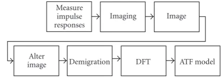
A block diagram outlining the required signal processing steps from the impulse responses to the ATF model is given in
Figure 4. It is to be emphasised that the ATFs contain neither reflections from other walls in the corridor hall nor the direct sound.
3. TRANSFER FUNCTION MODEL
The general model of a transfer function can be written as a rational function of the form
H(s)=B(s)
A(s)= M
m=0b[m]sm
N
n=0a[n]sn
, (7)
wheres = jωandBandAare the polynomials with coeffi
-cientsb[m]anda[n], respectively.
IfH(ω[k]) is the ATF to be modelled, the model is
ob-tained from the following equation error:
min
b,a
k
wω[k] Hω[k] Aω[k] −Bω[k] 2, (8)
whereB(ω[k]) andA(ω[k]) are the values of the numerator
and denominator of (7) evaluated at the discrete frequency
pointsω[k] determined by the DFT grid points. w(ω[k]) is
an optional weight function used to give greater emphasis to
certain frequencies. Equation (8) results in a system of linear
equations in the polynomial coefficientsa[n] andb[m] that
can be solved by matrix inversion in the least-squares sense
[19,20].
The weight function was defined as follows:
wω[k] =
⎧ ⎨ ⎩
0 for 0.97ωmax< ω[k]<0.03ωmax,
1 for 0.97ωmax≥ω[k]≥0.03ωmax.
(9)
The low weight at the extreme ends of the frequency band
afford the algorithm a high degree of freedom in that region.
An important and difficult issue is the order selection
Ma
gn
it
u
d
e
0 1 2 3 4
0 1000 2000 3000 4000 5000 6000 7000 8000 Frequency (Hz)
(a)
Phase
(
Æ
)
-180 0 180
0 1000 2000 3000 4000 5000 6000 7000 8000 Frequency (Hz)
(b)
Figure5: Typical (a) magnitude and (b) phase of measured room transfer function in the corridor hall.
in excess of a thousand coefficients [21, 22] for both the
numerator and denominator. The reasons are the numer-ous peaks and dips caused by the complex summation of many eigenmodes with quasirandom phases as discovered by
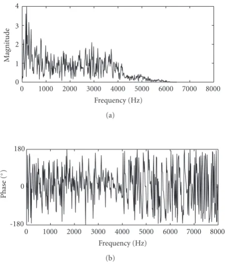
Schroeder [23]. As an example, Figure 5shows the
magni-tude and phase response of the room transfer function in the corridor hall (not just the single wall!). Since the average fre-quency spacing between adjacent dips and adjacent peaks is
equal [23], it would seem that the order of numerator and
de-nominator polynomials should also be approximately equal at least for the case of the whole room transfer function.
For the purpose of modelling the ATFs from the single augmented wall, the required model orders are much smaller and it proved feasible to model the entire frequency band
without resorting to subbands [24]. For reasons of
simpli-fication, the order of the numerator and denominator
poly-nomials was kept equal (N=M). Thus, if in the remainder
of the paper a model orderNis quoted, the actual total order
of the model isN+M=2N.
4. RESULTS
The following cases for the groups of eleven receiver posi-tions have been investigated:
(A) in front of the closet (z=0.5 m);
(B) in front of the closet (z=1.5 m);
(C) in front of the electrical distribution box; (D) in front of a homogenous wall section;
(D) (C) (B)
(A)
Array +Source
+O
Figure6: Extract ofFigure 2showing the positions of some of the cases considered.
(E) the same as (C) but with reflections from the electrical distribution box only;
(F) the direct sound at the positions of (B), (C), and (D).
Case (A) is at 0.5 m, whereas all other cases are at 1.5 m above
the lower array edge. Some of the positions of the diff
er-ent cases are shown inFigure 6. Each case consists of eleven
(33 for the direct sound) ATFs from the receiver positions at
0.05 m intervals on a horizontal line. The ATFs of the direct
sound in case (F) have been obtained directly from the orig-inal impulse response measurements. All other ATFs have been obtained from the impulse responses after demigration. Where appropriate, each case has been considered with all
three wall configurations listed inSection 2.2. For example,
case (C-3) refers to the ATF at the eleven positions in front of where the electrical distribution box would be, but the elec-trical distribution box has been removed and the wall is
ho-mogenously flat.Figure 7shows the impulse responses used
for the ATFs in cases (B), (C), and (D) in all three wall con-figurations (1), (2), and (3).
4.1. Example ATFs
Figure 8toFigure 10show typical magnitude and phase re-sponses of the demigrated ATF and its model for one receiver
position of case (C) in all three different wall configurations
(1), (2), and (3).
What the three figures clearly show is how the complex-ity of the ATF is decreasing as the structural details of the reflecting wall are decreasing. The general characteristics in
Figure 8 are very similar to those inFigure 9, yet the for-mer shows larger fluctuations within small frequency bands, which is to be expected due to interference between multi-ple reflections. Also, in accordance with expectation is that
Figure 10exhibits the most smooth magnitude and partic-ularly phase response of all three figures. It is also worth noting that the complexity of the ATF in the three figures is
much smaller than that inFigure 5. However, the chosen
or-der of the model is not yet sufficient to model all the details in
the ATFs. This can be seen particularly well by the spurious
spikes at approximately 1.2, 2.7, and 3.1 kHz inFigure 9.
4.2. Estimating the required model order
The error between the ATF and its model is defined by(N).
Ti
m
e
(m
s)
16 14 12 10 8
-3.5 -3 -2.5 -2 -1.5 -1 -0.5 0 0.5 1 1.5 x(m)
(a)
Ti
m
e
(m
s)
16 14 12 10 8
-3.5 -3 -2.5 -2 -1.5 -1 -0.5 0 0.5 1 1.5 x(m)
(b)
Ti
m
e
(m
s)
16 14 12 10 8
-3.5 -3 -2.5 -2 -1.5 -1 -0.5 0 0.5 1 1.5
(B) (C) (D)
x(m) (c)
Figure7: Demigrated impulse responses atz=1.5 m used for the ATFs, (a) configuration (1), (b) configuration (2), and (c) configu-ration (3). The vertical lines indicate the groups of eleven impulse responses used for cases (B), (C), and (D).
error formulation of (8) and is given by
(N)=
kwω[k] Hω[k] −BNω[k] ANω[k] 2
kwω[k] Hω[k] 2
,
(10)
with w(ω[k]) defined in (9). The numerator in the above
equation is the weighted sum of the squared amplitude dif-ferences between the ATF and its model and the denomina-tor is the weighted sum of the squared magnitude of the ATF. The latter serves as a normalisation factor such that the error
(N) is independent of the absolute magnitudes in the
dif-ferent ATFs. The required model order for a particular
case-configuration pair is then defined as the orderNat which the
error(N) falls below a predefined threshold. Unfortunately,
defining such a threshold is inevitably a subjective matter be-cause it depends on the desired accuracy of the model.
A practical problem that occurred when trying to find a
threshold was that(N) is not necessarily a function that is
monotonously decreasing before asymptotically approaching
a constant value forNlarge enough.Figure 11(a)shows(N)
for all eleven ATFs of case (C-3), where it is evident that the
M
ag
nitude
0 0.5 1 1.5
0 1000 2000 3000 4000 5000 6000 7000 8000 Frequency (Hz)
(a)
Phase
(
Æ
)
-180 0 180
0 1000 2000 3000 4000 5000 6000 7000 8000 Frequency (Hz)
(b)
Figure8: Case (C-1): (a) magnitude and (b) phase of ATF from demigration (solid line) and its model withN =31 (dashed line). Magnitude and phase of model have an offset for better compara-bility.
M
ag
nitude
0 0.5 1 1.5
0 1000 2000 3000 4000 5000 6000 7000 8000 Frequency (Hz)
(a)
Phase
(
Æ
)
-180 0 180
0 1000 2000 3000 4000 5000 6000 7000 8000 Frequency (Hz)
(b)
M
ag
nitude
0 0.5 1 1.5
0 1000 2000 3000 4000 5000 6000 7000 8000 Frequency (Hz)
(a)
Phase
(
Æ
)
-180 0 180
0 1000 2000 3000 4000 5000 6000 7000 8000 Frequency (Hz)
(b)
Figure10: Case (C-3): (a) magnitude and (b) phase of ATF from demigration (solid line) and its model withN =31 (dashed line). Magnitude and phase of model have an offset for better compara-bility.
errors shoot up at discrete values ofN. The reason for this
behaviour is that the ATF model is optimum for a
particu-lar value ofN but there is no guarantee that a lower-order
model does not have a smaller error value, and further the
difference between the output error in (10) and the equation
error in (8) may also contribute to the problem. It is also seen
in the figure that forNlarge enough, the problem no longer
occurs.
In order to circumvent these problems, a modified error
function(N) is introduced as follows:
(N)= 1
N
N
n=1
(n). (11)
The modified error of the model of orderNis therefore the
average of the errors of all models with orders from 1 toN.
This modification is quite arbitrary but has been introduced solely to render the thresholding process more robust. It did result in a monotonously decreasing function that asymp-totes a constant value for all the cases investigated. For all
eleven ATFs of case (C-3),(N) is shown inFigure 11(b). It
can be argued that a fluctuating behaviour of(N) is caused
by the complexity of the ATF to be modelled, and hence the model order is too small and must be increased. Finally, the
required model order was recorded as the value ofN, where
(N) ≤ 0.1. This particular value was determined
experi-mentally and was found to (i) guarantee no visual difference
(
N
)
0 0.2 0.4 0.6 0.8 1
0 50 100 150 200
N (a)
¼
(
N
)
0 0.2 0.4 0.6 0.8
0 50 100 150 200
N
(b)
Figure11:(N) and(N) for all eleven ATFs of case (C-3).
between model and actual ATF on the scale used inFigure 8
toFigure 10and (ii) to ensure that(N) does not shoot up
again for larger values ofNat any receiver position.
The results for the required order are expressed as mean and standard deviation between the eleven ATFs for each case
and configuration and are shown inTable 1.
5. DISCUSSION
FromTable 1, a general observation is that the highest orders for each wall configuration are mainly required for cases (B) and (C). In fact, for both these cases, the results are very sim-ilar for wall configurations (1) and (2). For case (D), where the receivers are positioned in front of a homogenous wall section, the required order is larger in cases (D-1) and (D-2) than in cases (D-3), albeit only slightly for (D-2). This sug-gests that the scattering from objects such as the electrical distribution box and the columns influence the ATFs at these positions.
For wall configuration (3), that is, the homogenous flat wall, the required mean order is 83 with a standard deviation of 15, the result for case (B-3) is almost 50% lower than for cases (C-3) and (D-3).
Table1: MeanNand standard deviationσ(N) of the ATF model order (over the set of eleven ATFs) for the different cases and configurations.
Case (A-1) (A-2) (B-1) (B-2) (B-3) (C-1) (C-2) (C-3) (D-1) (D-2) (D-3) (E) (F)
N 101 79 263 175 65 222 164 91 172 104 93 63 25
σ(N) 24 19 52 16 15 46 25 15 43 29 24 30 13
of the ATF is the most position dependent because of the amount of details present.
The results for case (A) are rather inconsistent with those from the other cases. The mean order is much lower, and in particular when compared to case (B) whose receiver positions are also in front of the closet. The reason for this is currently unknown.
For case (E), which contains reflections from the electri-cal distribution box only, the mean order is 63. Comparing with case (C-2) at the same positions in front of the wall, the standard deviation is roughly the same, but the presence of the entire wall increases the mean model order to 164.
For the direct sound (case (F)), the required order is on average 25. The figures quoted by Greendfield and
Hawksford [25] for the modelling of loudspeaker transfer
functions are roughly twice as large, however, due to the dif-ferent methodologies employed, a direct comparison is in-congruous. At any rate, the transfer function of the loud-speaker source is included in the ATFs of cases (A) to (E). In order to obtain the order of the ATF from the reflecting objects only, the order of the loudspeaker transfer function should be subtracted from the numbers listed. The lowest mean order thus obtained for a completely flat wall is 40 for case (B-3).
It is to be noted that the obtained model orders depend
on the efficiency of the transfer function modelling
algo-rithm and also on the value chosen for the error criterion.
The relative values for the model orders are therefore more meaningful and objective than the absolute values. The main findings from this paper can then be summarised as follows. The complexity (in terms of ATF model order) of sound re-flections from a physical wall comprising a number of de-tails is between two to three times higher than that of a ho-mogenous flat wall and varies by roughly 25% between re-ceiver positions. Further, the required model order for the physical homogenous flat wall is still relatively large. With a mirror image source model, the wall would be modelled as
a single planar surface and would require one coefficient in
the case of frequency-independent acoustic impedance and a slightly larger order to model the usually smooth varia-tion with frequency. It seems very unlikely that the
fluctu-ations inFigure 10 are only caused by acoustic impedance
variations.
The applications of the acoustic imaging process,
pre-sented in [13] and the present paper, to room acoustics are
the following. The method can serve as a tool to investigate
sound reflection from different reflecting object (e.g., wall)
details without the requirement of physically constructing the object and measuring its sound reflections in an
ane-choic chamber. The results have shown that reflections from objects, whose size is in the order of the shortest acoustic wavelength, are present in the room impulse response since otherwise the object would not appear in the acoustic image. In terms of wave-equation-based room acoustic models such
as finite elements, boundary elements or finite differences,
the message is that leaving out objects of the size of the acous-tic wavelength in question can potentially introduce signifi-cant errors, from both objective parameters and perceptual
point of view. An example is the increased “diffusion” offered
by the object details as compared to larger planar surfaces. It is conceivable that the presented method can be extended to quantify these errors objectively.
For room acoustic models based on geometrical acous-tics, the results from the macroscopic flat wall with fre-quency-dependent reflectivity properties reinforce the im-portance of incorporating and assigning a nonzero value for
the diffusion/scattering coefficient even to planar surfaces.
Further, comparing the complexity of the ATF from the ge-ometrical acoustics model with that from the acoustic image
can aid in the task of accurately modelling diffraction and
scattering through surface and edge sources. This in turn can potentially help to improve the physical accuracy versus com-putational complexity dilemma encountered in room acous-tics modelling. A further interesting avenue is the perceptual comparison between the reflections from the macroscopic flat wall in this paper and the flat wall from a geometrical acoustics model.
6. CONCLUSION
The modelling of acoustic transfer function (ATF) from the reflections of single objects has been performed. The purpose was to investigate the complexity of the reflections from real physical objects. The ATFs have been obtained by demigrat-ing the acoustic image of the reflectdemigrat-ing objects, consistdemigrat-ing of a corridor wall with a number of details such as columns, a closet, and an electrical distribution box. The original acoustic image has been augmented first by simplifying it and then by replacing larger objects with homogenous wall sections.
The ATFs to be modelled stem from various receiver po-sitions in front of the wall. The required model order has been estimated from the error between modelled and actual ATFs. It was found that the maximum and minimum
to-tal model orders 2N are 526 and 126, respectively. For the
for the homogenous flat wall was 130. Finally, the order 2N of the loudspeaker transfer function, which is implicitly in-cluded in the ATF, was estimated as 50. This figure would need to be subtracted from the above-quoted numbers.
The results in this paper confirmed the applicability of some of the practices in current room acoustics modelling and the method itself can be used to further understand and improve the modelling of reflections from real physical objects.
ACKNOWLEDGMENTS
The authors thank three anonymous reviewers and the As-sociate Editor Aki H¨arm¨a for valuable remarks about the manuscript text.
REFERENCES
[1] J. B. Allen and D. A. Berkley, “Image method for efficiently simulating small-room acoustics,”Journal of the Acoustical So-ciety of America, vol. 65, no. 4, pp. 943–950, 1979.
[2] H. Kuttruff,Room Acoustics, chapter 2, Spon Press, London, UK, 4th edition, 2000.
[3] M. Vorl¨ander, “Simulation of the transient and steadystate sound propagation in rooms using a new combined ray-trac-ing/image-source algorithm,”Journal of the Acoustical Society of America, vol. 86, no. 1, pp. 172–178, 1989.
[4] I. A. Drumm and Y. W. Lam, “The adaptive beam-tracing al-gorithm,”Journal of the Acoustical Society of America, vol. 107, no. 3, pp. 1405–1412, 2000.
[5] A. J. Berkhout, D. de Vries, J. Baan, and B. W. van den Oetelaar, “A wave field extrapolation approach to acoustical modeling in enclosed spaces,”Journal of the Acoustical Society of America, vol. 105, no. 3, pp. 1725–1733, 1999.
[6] B.-I. L. Dalenb¨ack, “Room acoustic prediction based on a uni-fied treatment of diffuse and specular reflection,”Journal of the Acoustical Society of America, vol. 100, no. 2, pp. 899–909, 1996.
[7] B.-I. L. Dalenb¨ack, “Verification of prediction based on ran-domized tail-corrected cone-tracing and array modeling,” in
Proceedings of the 137th ASA Meeting, 2nd Convention of the European Acoustics Association and 25th German Acoustics DAGA Conference, Berlin, Germany, March 1999.
[8] J. J. Embrechts, “Broad spectrum diffusion model for room acoustics ray-tracing algorithms,”Journal of the Acoustical So-ciety of America, vol. 107, no. 4, pp. 2068–2081, 2000. [9] Y. W. Lam, “A comparison of three diffuse reflection modeling
methods used in room acoustics computer models,”Journal of the Acoustical Society of America, vol. 100, no. 4, pp. 2181– 2192, 1996.
[10] R. R. Torres, U. P. Svensson, and M. Kleiner, “Computation of edge diffraction for more accurate room acoustics aural-ization,”Journal of the Acoustical Society of America, vol. 109, no. 2, pp. 600–610, 2001.
[11] U. P. Svensson, R. I. Fred, and J. Vanderkooy, “An analytic sec-ondary source model of edge diffraction impulse responses,”
Journal of the Acoustical Society of America, vol. 106, no. 5, pp. 2331–2344, 1999.
[12] A. Farina, “Introducing the surface diffusion and edge scat-tering in a pyramid-tracing numerical model for room
acous-tics,” inProceedings of the 108th Audio Engineering Society Con-vention (AES ’00), Paris, France, February 2000.
[13] M. Kuster, D. de Vries, E. M. Hulsebos, and A. Gisolf, “Acoustic imaging in enclosed spaces: analysis of room, geometry mod-ifications on the impulse response,”Journal of the Acoustical Society of America, vol. 116, no. 4, pp. 2126–2137, 2004. [14] D. de Vries, N. Joeman, and E. Schreurs, “Measurement-based
simulation and analysis of scattering structures,” in Proceed-ings of the Forum Acusticum, Budapest, Hungary, August 2005. [15] D. J. Verschuur, private communication, 2006.
[16] M. Tygel, J. Schleicher, and P. Hubral, “A unified approach to 3-D seismic reflection imaging, part II: theory,” Geophysics, vol. 61, no. 3, pp. 759–775, 1996.
[17] E. W. Start, V. G. Valstar, and D. de Vries, “Application of spa-tial bandwidth reduction in wave field synthesis,” in Proceed-ings of the 98th Audio Engineering Society Convention, Paris, France, February 1995.
[18] D. de Vries, M. Kuster, and E. Hulsebos, “Analyzing the influ-ence of design modification on the room response by acousti-cal imaging,” inProceedings of the International Symposium on Room Acoustics: Design and Science (RADS ’04), Hyogo, Japan, April 2004.
[19] E. C. Levy, “Complex-curve fitting,”IRE Transactions on Auto-matic Control, vol. 4, no. 3, pp. 37–44, 1959.
[20] Y. Haneda, S. Makino, and Y. Kaneda, “Common acoustical pole and zero modeling of room transfer functions,” IEEE Transactions on Speech and Audio Processing, vol. 2, no. 2, pp. 320–328, 1994.
[21] J. Mourjopoulos and M. A. Paraskevas, “Pole and zero mod-eling of room transfer functions,”Journal of Sound and Vibra-tion, vol. 146, no. 2, pp. 281–302, 1991.
[22] M. Karjalainen, T. Paatero, J. N. Mourjopoulos, and P. D. Hatziantoniou, “About room response equalization and dere-verberation,” inProceedings of IEEE Workshop on Applications of Signal Processing to Audio and Acoustics (WASPAA ’05), pp. 183–186, New Paltz, NY, USA, October 2005.
[23] M. R. Schroeder, “Statistical parameters of the frequency re-sponse curves of large rooms,”Journal of the Audio Engineering Society, vol. 35, no. 5, pp. 299–306, 1987.
[24] M. Sch¨onle, U. Z¨olzer, and M. Fliege, “Modeling of room impulse responses by multirate systems,” in Proceedings of the 93rd Audio Engineering Society Convention, San Francisco, Calif, USA, October 1992.
[25] R. Greenfield and M. O. Hawksford, “Efficient filter design for loudspeaker equalization,”Journal of the Audio Engineering So-ciety, vol. 39, no. 10, pp. 739–751, 1991.
Martin Kusterobtained a B.Eng. degree in electroacoustics from the University of Sal-ford, UK, in 2001 and an M.S. degree in ap-plied physics from Delft University of Tech-nology, The Netherlands, in 2003. He joined the Queen’s University Belfast in Septem-ber 2004 to work on a collaborative project with a digital entertainment company, in the framework of which he undertakes re-search into room acoustic (inverse)
Diemer de Vrieswas born January 3, 1945, in Weststellingwerf, Friesland, The Nether-lands. He received his M.S. degree from Delft University of Technology in 1971 on a thesis on architectural acoustics. During his career as a University Researcher, he worked on several projects in room acoustics, build-ing acoustics, and seismic signal process-ing. In 1984, he received a Ph.D. degree on a thesis in the latter field. He now