Circular contour retrieval in real-world conditions by higher order statistics and an alternating-least squares algorithm

R E S E A R C H

Open Access

Circular contour retrieval in real-world conditions

by higher order statistics and an alternating-least

squares algorithm

Haiping Jiang, Julien Marot, Caroline Fossati and Salah Bourennane

Abstract

In real-world conditions, contours are most often blurred in digital images because of acquisition conditions such as movement, light transmission environment, and defocus. Among image segmentation methods, Hough transform requires a computational load which increases with the number of noise pixels, level set methods also require a high computational load, and some other methods assume that the contours are one-pixel wide. For the first time, we retrieve the characteristics of multiple possibly concentric blurred circles. We face correlated noise environment, to get closer to real-world conditions. For this, we model a blurred circle by a few parameters–center coordinates, radius, and spread–which characterize its mean position and gray level variations. We derive the signal model which results from signal generation on circular antenna. Linear antennas provide the center coordinates. To retrieve the circle radii, we adapt the second-order statistics TLS-ESPRIT method for non-correlated noise environment, and propose a novel version of TLS-ESPRIT based on higher-order statistics for correlated noise environment. Then, we derive a least-squares criterion and propose an alternating least-squares algorithm to retrieve simultaneously all spread values of concentric circles. Experiments performed on hand-made and real-world images show that the proposed methods outperform the Hough transform and a level set method dedicated to blurred contours in terms of computational load. Moreover, the proposed model and optimization method provide the information of the contour grey level variations.

Keywords:blurred circle, concentric circles, correlated noise, higher-order statistics, ALS algorithm

1 Introduction

Blurred contours occur very often in images, owing to object movements, light transmission environment, illu-mination changes, defocus, optical instrumentation, etc. Light has recently been shed on the characterization of contours, regions, or objects which are not simply defined by a one-pixel wide contour [1,2].

Circle fitting problems can be applied to several industrial fields, such as the test of mechanical parts in manufacturing, and quality inspection for food industry. For these applications, the detected images are often affected by correlated Gaussian noise. Also, the expected objects may rely on a surface which yields an image background that can be assimilated to correlated Gaus-sian noise. In these cases, how to effectively estimate

circle or circle-like contour is an interesting problem. Several methods were proposed in the last few years.

First, region-based segmentation methods aim at dis-tinguishing between sets of pixels of the image, referring to properties such as color, texture [3], or object reparti-tion which yields mathematical morphology methods [4,5]. Unsupervised classification was recently performed with Hidden Markov Random Fields (HMRF) [2].

Second, contour-based segmentation methods aim at retrieving the sets of pixels which form the contours themselves. Generalized Hough transform (GHT) [6] method detects the object’s outline by organizing an accumulator-type parameter space and mapping each point in the image into a surface in the parameter space. Although it is robust to partial or slightly deformed shapes and tolerant to noise, its computa-tional load increases dramatically with the number of edge points. Besides, GHT also requires a huge storage

* Correspondence: [email protected]

CNRS-UMR 6133/Fresnel Institute-Ecole Centrale Marseille, D. U. de Saint-Jérôme, 13397 Marseille Cedex 20, France

space even if hierarchical search is adopted. Ordinary or total least-squares methods for circle fitting seek to minimize the squares sum of error-of-fit with respect to measures [7,8]. Using geometric fitting [7], error tances are defined with the orthogonal, or shortest, dis-tances from given points to the geometric feature to be fitted. In [8], a least-squares fitting approach is pro-posed. It is based on the hypothesis that a set of circular arcs extracted from the image is related to a set of cir-cles contained in a model by translation, rotation, and scaling. These methods are restricted to one-pixel wide contours and are sensitive to noise. A recent model for active contours based on the techniques of curve evolu-tion considers blurred contours as contours which are not necessarily defined by gradient. It was adapted from the level set paradigm [9], and was proposed to segment contours“without edges”[1]. In [10], a solution combin-ing the geodesic active contour approach and interpola-tion constraints is provided to improve the convergence of level sets in the case where the image is noisy and the contours are not well defined. The main weakness of this method is that thea priori knowledge of interpo-lation points is required, so that the method is not entirely blind. More recently, in [11], a level set-type method for segmentation in harsh conditions such as high level noise, using a shape prior and a deformable contour, is proposed. Still, it is not entirely blind. In [12], the authors present a novel fast model for active contours to detect objects in an image, based on techni-ques of curve evolution. The proposed model can detect objects whose boundaries are not necessarily defined by gradient. Considering contours which are not necessarily defined by gradient constituted a very valuable advance but these methods suffer from an elevated computa-tional load. An effort has been recently dedicated to the reduction of the computational load of level set algo-rithms [13], but no specific effort is done to face blurred contours. It is feasible to establish the analogy between source localization in array processing [14,15] and con-tour detection in image processing. Still in the field of contour-based segmentation methods, Aghajan et al. [16,17] first proposed to transfer array processing meth-ods to the field of image processing with a view to char-acterize straight lines. Their basic idea was to associate the processed image with a virtual linear antenna. Then, Marot et al. [18,19] extended this method to multiple circle retrieval while proposing a virtual circular antenna. Virtual antennas and associated subspace-based methods of array processing are restricted to one-pixel wide line [17] retrieval, and one-pixel wide circle retrie-val [18] in a non-correlated Gaussian noise environ-ment. The purpose of this article is the detection of circles in conditions which are as close as possible to real-world ones. We propose to detect multiple

concentric circles which may be blurred. More precisely, we look for the following parameters of interest: the center coordinates, the radius, and the spread. We pro-pose a method based on higher-order statistics to retrieve radius values in a correlated noise environment, and an alternating least-squares (ALS) optimization method [20] to retrieve the spread parameters of con-centric contours. Thereby, we overcome the limitations of the Hough transform [6] which does not characterize the contour blur, we propose fast methods which char-acterize the expected contours by a few parameters, as opposed to level set type methods [1] which rely on a computationally costly evolution of the active contour. We also improve previous studies which transposed array processing methods into the image processing community [16,18,21-24] by considering contours which are no longer one-pixel wide. The remainder of the arti-cle is organized as follows: Section 2 states the problem of detecting multiple circles in a noisy environment. We propose a model for the grey level variations of a blurred circle. In Section 3, we explain how to locate the center of the expected blurred circles. In Section 4, we derive the models for the signals which are obtained when concentric blurred circles are present, and we apply generation on the circular antenna. In Section 5, we consider multiple radii estimation: first, we adapt the TLS-ESPRIT (Total Least Squares Estimation of Signal Parameters by Rotational Invariance Techniques) method [15] based on second-order statistics in non-correlated noise environment; second, we propose a new version of TLS-ESPRIT method, based on higher-order statistics, which faces correlated noise. In Section 6, we propose an ALS method, to retrieve the spread values of concentric circles. The ALS process permits to estimate recursively all spread values by taking into account the other estimated values. In Section 7, we propose a dis-cussion about the validity domain of the proposed form-alism, and present typical results that can be obtained by the proposed methods in this domain of validity. After concluding the paper in Section 8, we develop some calculatory aspects and show how to retrieve the circle centers in an annexe (Section 9).

2 Problem statement

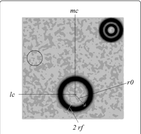
are imaged over a background whose regular texture is such that it can be considered as correlated noise. For instance, the treadmills for food products transportation have a regular structure. That is why, in this article, we aim at characterizing blurred circular contours in noisy environment, in particular in images which contain cor-related noise. For this, we provide a model for the image containing the expected circular blurred contours, called further in this article the processed image. We also provide a model for the grey level variations of the expected contours. Let I(l, m) be an N× Nrecorded image (see Figure 1). This image contains several blurred circles (two in the example of Figure 1) charac-terized by center coordinates {lc; mc}, a center radiusr0, and a width 2rf. The center radius r0 is defined by the location of the pixels which have maximum grey level value. These pixels define the center circle. Previous stu-dies [21-24] consider contours which are only one pixel-wide. In this article, a contour is no longer restricted to a one pixel-wide feature. A contour is defined by non-zero grey level values aside the center circle, at a maxi-mum distance rf on each side of the center circle. The image background is composed of pixels with value 0. In addition to the expected circles, an additive identi-cally distributed noise, whose grey level values follow a Gaussian distribution, impairs part of the pixels of the image. This noise may be correlated.

The variations of the grey level values aside the center circle are modeled as an exponential function of the dis-tance to the center circle. We expect that the

exponential distribution, for instance a Gaussian distri-bution, of the gray level values, facilitates the transfer of array processing methods to the considered parameter estimation issue. For one circle with the parameters cited above, the grey level valuesI(l,m) are then defined as follows:

I(l,m) = √G 2πσe

−(

(l−lc)2+ (m−mc)2−r0) 2

2σ2 (1)

wheresis a spread parameter: the largers, the slower the grey level values decrease aside the center circle.

Referring to Equation 1, √G

2πσ is the maximum gray level value. It holds for the pixels of the center circle.

The parameter Gis such that √ G 2πσmin

= 1in a

noise-free image, smin being the minimum spread value among all contours. The first step among the proposed algorithms consists in the retrieval of the center of the blurred circles. This is explained in the following section.

3 Retrieval of the center by signal generation on linear antennas

In real-world conditions, it is common that several con-tours are expected in the same image. We explain in this section how to retrieve the center coordinates of several blurred circles. We generate signal components

zlin(l), l = 1,..., N, on a linear antenna placed either at the left side or the bottom side of the image. The lth signal component, generated from thelth row, reads:

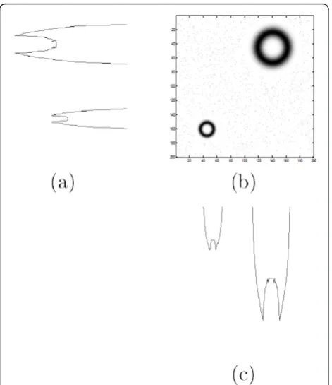
zlin(l) =Nm=1I(l,m)exp(−jμm), where μ is a genera-tion, or“propagation”parameter [16]. The non-zero sec-tions of the signals, as seen at the left and bottom sides of the image (see Figure 2), indicate the presence of cir-cles. Each non-zero section width in the left (respec-tively the bottom) side signal gives the height (respectively the width) of the corresponding expected contour. The middle of each non-zero section in the left (respectively the top) side signal yields the value of the centerlc(respectivelymc) coordinate of each circle. To associate thelc parameter of a given circle with itsmc parameter, we associate the non-zero sections which have same length in the left antenna and the bottom antenna signals.

This process is the first step of all proposed algo-rithms. Indeed, after detecting the center of the expected circles, a virtual circular antenna provides sig-nals which can be analyzed to retrieve the radius and spread of the blurred circular contours. The knowledge of the center coordinates permits to adapt a specific

Figure 1Image model and parameters characterizing a blurred circular contour: center coordinates {lc;mc}, radiusr0, and

signal generation technique and to estimate the other parameters of the contours. This is the purpose of the following sections.

4 Signal generation on circular antenna and signal models

In this section, we remind a signal generation process proposed in [18], and derive the signal model which holds for the signals generated out of an image contain-ing a circular blurred contour.

4.1 Virtual circular antenna

The basic principle of the circular antenna is to get, out of the two-dimensional processed image, a one-dimen-sional signal which can be analyzed by second-order or higher-order statistics. For this, we adapt the shape of the antenna to the shape of the expected contour. In [16,21,22], a linear antenna is adapted to get a linear phase signal out of an image containing (possibly slightly distorted) straight lines. In [18], circular con-tours are expected. Therefore, a circular antenna is adapted, so that a circular contour in the image yields a linear phase signal after signal generation on the antenna. As shown in Figure 3, the circular antenna is composed of S sensors equally distributed along a

quarter of circle which is centered on the center of the expected contour.

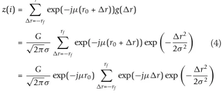
Each antenna sensor indexed by i corresponds to a signal component denoted by z(i). The signal compo-nents z(i), i = 1,..., S are computed out of the image through the formula of Equation 2:

z(i) =Ns

l=1

Ns

m=1 (l,m)∈Di

I(l,m) exp(−jμ√l2_+m2_),

(2)

whereDidenotes a direction for signal generation (see Figure 3); the expression (l, m) Î Di means that the summation over pixels (l,m) is performed along the sig-nal generationDionly; andμis a propagation coefficient which is set by the user.

4.2 Signal model for concentric circular contours

Let us consider a one-pixel wide circular contour, i.e.,I

(l, m) = 1 if

(l−lc)2+ (m−mc)2=r0 andI(l,m) = 0 otherwise. Referring to Equation 2, we get z(i) = exp (-jμr0)∀i. Asμhas a fixed constant value, this“constant speed” generation scheme yields signal components of same values.

To express I(l, m), we refer to Equation 1, and sim-plify it, denoting by Δr the shift between a pixel and the contour mean position. The blurred circular contour gray level variation is then

Figure 2 Center retrieval: (a) Signal generated on the left antenna; (b) processed image; (c) signal generated on the bottom antenna. Center retrieval by signal generation on linear antennas.

g(r) = √G 2πσ exp

−r2

2σ2

(3)

Referring to Equations 2 and 3, the generated signal components are formulated as

z(i) = rf

r=−rf

exp(−jμ(r0+r))g(r)

=√G

2πσ rf

r=−rf

exp(−jμ(r0+r)) exp

−r2

2σ2

=√G

2πσexp(−jμr0) rf

r=−rf

exp(−jμr) exp

−r2

2σ2

(4)

Following the results of the annexe (Section 9), we can turn the considered discrete calculation into a continu-ous case calculation:

z(i) =√G

2πσexp(−jμr0)

r=+∞

r=−∞ exp(−jμr) exp

−_2σr22

d(r) (5) Using the general formula of Equation 28, Equation 5 is rewritten as:

z(i) = exp(−jμr0) exp

−σ2μ2

2

. (6)

The intuition behind the approximation in Equation 5 is that, ifsis small enough compared with the number of pixels along the directionDiof signal generation, the discrete summation can be turned into an integral.

To fit the signal model of frequency retrieval methods, we adopt, instead of the fixed parameter μ, a propaga-tion parameter whose value depends on the sensor index. That is, we chooseμ=a(i- 1), whereais a con-stant. The propagation parameter is therefore variable, hence the denomination of the“variable speed” scheme which provides,∀i:

z(i) = exp(−jα(i−1)r0) exp

−σ2α2(i−1)2

2 . (7)

For a set of dconcentric circular contours, and taking into account an additive noise due to the presence of noise pixels, a signal componentz(i) reads:

z(i) = d

k=1

exp(−jα(i−1)r0k) exp

σ2

kα2(i−1) 2

2 +n(i). (8)

wheren(i) is a noise term. This also can be expressed as

z(i) =

d

k=1

βkexp(−jα(i−1)r0k) +n(i), (9)

with βk= exp

−σk2α2(i−1)

2

2 ,k= 1,. . .,d.

The signal components of Equation 9 form the vector

z= [z(1),z(2), ...,z(S)]T, where superscript“T” denotes transpose. As the signal vectorzin Equation 9 contains several harmonics, we aim at retrieving its parameters with a frequency analysis method. This is the purpose of Section 5.

4.3 Note about the number of sensors

The circular antenna is centered on the top-left corner of the sub-image selected from the processed image (see Figure 3). So, the maximum value of the contour center radius isNS, and the center circle of any circle is made

of at most πNS

2 pixels. So that every contour pixel has an influence on the generated signal, the circular

antenna should then have at least πNS

2 sensors.

5 Retrieval of the radii of concentric circles In this section, we consider the estimation of the radii of concentric circles, in two cases: when non-correlated Gaussian noise impairs the image, and when correlated Gaussian noise impairs the image. In the first case, we adapt TLS-ESPRIT method, which is based on second-order statistics. In the second case, we propose an improved version of TLS-ESPRIT, which faces corre-lated noise using higher-order statistics.

5.1 Second-order statistics for the estimation of the blurred circle radii

From Equation 9, we notice that the problem of radius estimation is similar to the retrieval of harmonics in sev-eral signal processing fields such as radar, sonar, com-munication. The resulting signal appears as multiple damped sinusoids with frequencies:

fk=−αr0k/2π (10)

To solve this problem, we adapt TLS-ESPRIT (Total least-squares-EStimation of Parameters by Rotational Invariance Techniques) algorithm [15]. TLS-ESPRIT algorithm requires the estimation of the covariance matrix of several snapshots. There are no time-depen-dent signals. So, the question arises as how a sample covariance matrix can be formed. This can be done as follows [16]: from the observation vector we build P

subvectors of lengthM withd<M≤S-d+ 1:

matrix that is performed in TLS-ESPRIT algorithm. We obtain thenP=S+ 1 - Msnapshots. Grouping all sub-vectors obtained in matrix form, we get ZP = [z1,...,zP], where

zp=AMs+np, p= 1,. . .,P. (11)

AM= [a(r01),...,a(r0d)] is a Vandermonde type matrix of sizeM ×d: theith component ofa(r0k) is exp(-ja(i -1)r0k).sis a lengthdvector equal to [b1,b2, ...,bd]Tand

np= [n(p),...,n(p+M- 1)]T.

The signal model of Equation 11 suits TLS-ESPRIT method, a subspace-based method that requires the dimension of the signal subspace, i.e., in this problem, the number of concentric blurred circles. Minimum descrip-tion length (MDL) criterion [25] estimates the dimension of the signal subspace [16] from the eigenvalues of the covariance matrix. TLS-ESPRIT is applied on the mea-surements collected from two overlapping subarrays, and falls into two parts: the covariance matrix estimation and the minimization of a total-least-squares criterion. The estimated radius values are obtained as [15]:

ˆ

r0k= −

1 α Im

ln

λk

|λk|

, k= 1,. . .,d (12)

where Im denotes imaginary part, lk,k= 1,...,d are the eigenvalues of a diagonal unitary matrix. It relates the measurements from the first subarray with the mea-surements resulting from the second subarray. The values of the radii of all concentric circles are known at this point, and can be used to retrieve the spread values. This is the purpose of Section 6.

In some cases, the noise which impairs an image is correlated. In the next section, we show how to take this into account.

5.2 Extension to correlated noise environment with higher-order statistics

In a correlated noise environment, we consider the esti-mation of the contour parameters by a higher-order sta-tistics method to suppress the noise [26]. The idea behind the proposed algorithm is based on the well-known cumulant property stating that the higher-order cumulants of a Gaussian variable are null [27]. In the following, we introduce a novel method, which is inspired by TLS-ESPRIT, but includes the computation of higher-order cumulants. As well as in the TLS-ESPRIT method, the signals generated out of the image are spatially smoothed, and these signals (see Equation 11) can be rearranged as follows

X(1)X(2)· · ·X(P)= ⎡ ⎢ ⎣

z1

.. .

zM

⎤ ⎥ ⎦=

⎡ ⎢ ⎣

z(1) z(2) · · ·z(N−M+ 1) ..

. ... . .. ...

z(M)z(M+ 1)· · · z(N) ⎤ ⎥

⎦ (13)

WhereM=S-P+ 1 andd<M≤S-d+ 1. For every snapshot, X(p) =AMs(p) +n(p), where p= 1, ...,P, AM = [a(r1),a(r2), ...,a(rd)] withkth column a(rk) = [1, exp (-jark),..., exp(-ja(M - 1)rk)]T, ands(p) = [b1,...,bd]T. A fourth-order cumulant matrix is then appropriately defined as

C_{X X},4={cum4(zi,zi,z∗i,z∗j)} i=1,...,M;

j=1,...,M. (14) Then, we propose a novel variant of TLS-ESPRIT algorithm. In order to follow the key steps of classical algorithm [15], we derive four (M- 1) × (M- 1) subma-trices:

C11={cum4(zi,zi,z∗i,z∗j)}

i=1,...,M−1;

j=1,...,M−1 C12={cum4(zi,zi,z∗i,z∗j)}

i=1,...,M−1;

j=2,...,M

C21={cum4(zi,zi,z∗i,zj∗)}j=1,i=2,......,M,M−;1. C22={cum4(zi,zi,z∗i,z∗j)}

i=2,...,M;

j=2,...,M.

(15)

We reconstruct these four submatrices and apply sin-gular value decomposition (SVD) operation. Some detection methods, such as MDL, can be used to esti-mate the number of sources by applying the eigen-decomposition operation for the cumulant matrix in place of the covariance matrix.

The overall process based on higher-order cumulant can be summarized as follows:

(1) Form the matrix C_{X X},4 by Equations 13 and 14; (2) Generate four submatrices from Equation 15 and reconstruct the matrixCas:

C=

C11C12 C21C22

(16)

(3) Perform SVD operation with C=EΛEH, whereΛ =diag(l1,...,l2(M-1)) with the eigenvalues l1≥ ...≥ ld≥ ... l2(M-1), and l1, ..., ld correspond to the signal subspace.

(4) LetE1 be the 2(M - 1) × d upper-left matrix ofE andE2 be 2(M - 1) × d matrix obtained by deleting the first row of matrixE. Carry out the eigen-decomposition

EH₁

EH₂ E1E2

=FFFH;

F=

F11F12 F21F22

(5) Extract the submatricesF₁₂andF₂₂, then find the eigenvalues {gk} of −F12F−221.

(6) Obtain each radius value as

r0k= −

1

The circular antenna also permits to distinguish parti-cular cases while estimating the center coordinates (see Section 3). Indeed some particular cases may appear in this process: if no zero section appear, either the image is noisy or the contributions of all contours are added. A threshold depending on the maximum value of the modulus of the signal is applied. If there is no contour in the image, and only noise, no dominant values will appear in the modulus of the signal and no threshold can be applied. If there is noise and a contour which is not a circle, the linear antennas yield a center for this contour. Then, the algorithms presented in the current section which follow signal generation on circular antenna yield absurd results, which indicates that the detected contour is not a blurred circle. The case where several circles are present was partially solved: some solutions involving a circular antenna were proposed for circles with same diameter (see [18]), and for the case where two circles overlap (see [19]).

The values of the radii are now available, which per-mits to build a signal model for the estimation of the spread parameters. This is the purpose of the following section.

6 ALS optimization method for the estimation of the spread parameters

In the case where several blurred concentric circular cir-cles are present, dradius valuesr0k, k= 1,...,dand also

d spread values sk, k = 1,..., d must be estimated for each center. The spread values are included in the signal model proposed in Equation 8, as well as the radius values r0k, k = 1,..., d. The values r0k, k = 1,..., d are known at this point (see Section 5). Therefore, it is pos-sible to retrieve these spread values by minimizing the squared Frobenius norm of the difference between the model signal and the signal generated out of the image on the circular antenna. This is an optimization problem involving several unknowns. An ALS algorithm is an adequate solution for this problem and already led to good results in the field of image processing [20]. Therefore, we propose to obtain the spread parameters by minimizing a least square criterion between the sig-nal model proposed in Equation 8, and the sigsig-nal gener-ated from the image on the circular antenna. So, we start from the signalz= [z(1),z(2),...,z(S)]Twhose com-ponentsz(i) are defined in Equation 8. The valuesr0k,k = 1,...,dare used to obtain a model for the signal com-ponents zmodel(i) defined in Equation 8. Let us then denote byzmodelthe signal whose components arezmodel (i),i= 1,...,S, and let us denote byzimagethe signal gen-erated out of the image. With these notations, the vector of spread parametersscan be estimated as follows:

ˆ

σ = arg min

σ (||zmodel−zimage||

2₎

(17)

which can be expressed as:

ˆ

σ= arg min

σ (Jcircle(σ)) (18)

whereJcircledenotes the criterion to be minimized. The criterion Jcircle does not depend linearly on the vectorscontaining thedspread parameters to be esti-mated. Therefore, a linear optimization algorithm such as Newton method cannot be applied directly to get an estimate of the vector s. That is why, all components {s1, s2,..., sd} ofs are estimated successively. To take into account the dependence between all spread values, we adapt an ALS algorithm. In one iteration of the ALS algorithm, the spread parameters are estimated succes-sively. Once any spread value has been estimated, it must be taken into account for the estimation of the other spread values. So, this process is iterated. The ALS algorithm can be summarized in the following steps:

1.InitializationIt= 0:s0 = [0,..., 0]T 2.ALS loop:

Repeat until convergence, i.e., ||Jcircle||2 <, with > 0 prior fixed threshold,

(a) i. for k= 1 to d: adapt the Newton algo-rithm. We expect that Newton algorithm retrieves efficiently one parameter σIt

k, through

the following loop: setq= 0. Whileq<qstop: A.

σIt

k =σkIt−λ

∂(Jcircle(σIt))

∂σIt k

(19)

B.q¬q+ 1.

where l is the step for the descent, and

qstop is thea priorifixed last iteration index of the loop.

ii. Update the kth element of sIt with the value of σ_kIt obtained at iterationqstop; iii. Incrementk;

(b) Increment It;

3.output: σItstop with It_stop being the last iteration

after convergence of the ALS loop. In Equation 19,

the partial derivative ∂(Jcircle(σ It₎₎

∂σIt

k

is expressed as

∂(Jcircle(σIt))

∂σIt

k

= 2∗∂(zmodel) ∂σIt

k

∗(zmodel−zimage)(20)

where

∂(zmodel) ∂σIt

k

=−σk(i−1)2α2exp(−jα(i−1)r0k) exp

−σk2(i−1)2α2

2 (21)

The proposed ALS optimization algorithm provides the spread values. With the knowledge of the center coordinates, the radii and the spread values, the expected contours are entirely characterized. In the fol-lowing section, we discuss the domain of validity of the proposed methods, and exemplify them on hand-made and real-world images.

7 Discussion and results

In this section, experiments are performed on a PC running Windows equipped with a double CPU at 3.00 GHz. Unless specified, the experiments are performed in these condi-tions: we apply the proposed methods on images with size 200 × 200 pixels or more. To retrieve the center of the cir-cles, we apply a signal generation scheme on linear anten-nas while setting a propagation parameterμ= 10-3. To estimate the radius (and spread in the case of blurred cir-cles) of the expected contours, we use a circular antenna composed ofS= 500 sensors, and we apply variable speed propagation scheme with a propagation parametera= 2 10-3. While running Newton algorithm, the descent coeffi-cient isl= 0.5, and 200 iterations are performed.

First, we characterize blurred circles in a noise-free or non-correlated Gaussian noise environment. Second, we characterize possibly blurred circles in a correlated noise environment. We compare the proposed method with Chan and Vese method [1]. The parameters which are adequate when running this method are as follows: the level is 0.7, the number of iterations is 50, and weighting terms for the energy areμCV= 0.03 * 2552,νCV= 0, and

lCV1=lCV2 = 1. In Section 7.1, we discuss the approxi-mation which provides an integral out of a sumapproxi-mation and which yields the proposed signal model for blurred circular contours in the annexe (Section 9); in Section 7.2, we study various cases of blurred circle retrieval and the computational load of proposed and comparative methods; in Section 7.3, we study the case where corre-lated noise impairs the image and blurred concentric circles are present in the image; and in Section 7.4 we analyze two images coming from a real-world context to quantify the effect of a Dove prism on a light beam.

7.1 Discussion about the approximation which yields an integral from a discrete summation

In this section, we discuss the approximation which yields Equation 29 in the annexe (Section 9). This is

done with a view to giving an interval for the para-meters of the problem where this approximation is valid. This permits to justify the experimental conditions chosen in the following subsections of this section. For a given propagation parameterμ, the parameters of inter-est in Equation 29 are the half number of pixelsrf on which the summation is performed, and the spread parameters. We expect that the higherrfand the smal-ler s, the smaller the difference between the two terms of Equation 29. We choose as maximumrfthe valuerf = 78, which is coherent with the size chosen for most of the images. This value is attained as soon as the sub-image containing the expected quarter of circle has size 55 × 55, which is less than N. Viewing the size of the images, we fix the maximum value ofstos= 8.

In Section 4.2, a variable speed propagation scheme is chosen to fit the signal model of a frequency retrieval method. We setμ=a(i- 1),∀i= 1,...,S. Fora= 2 10 -3

andS= 500, the extreme values of μare then 0 and 1. Therefore, for the propagation parameter μ= 1, for 100 values ofrfequi-spaced between 42 and 78, and for 100 values ofs equi-spaced between 1 and 8, the relative error is computed as follows:

Er= |L−R|

min(L,R) (22)

where _L and _R are the left and right terms of Equa-tion 29, respectively, in the calculaEqua-tions developed in the Annexe (Section 9).

In the conditions of Figure 4a, the values of spread parametersare the highest, which draws us away from the best conditions for the validity of Equation 29. How-ever, we notice that, as soon as the parameterrfis larger than 65, which is coherent with the size of the

60 70

80

0 5 10

0 0.1 0.2 0.3 0.4 0.5

r f (a)

σ ₄₀

60 80

0 2 4 6 0 2 4 6 8

x 10−5

r f (b)

σ

Figure 4Relative error valuesErfor: (a)sÎ[1:8] andrfÎ[62:

78]; (b)sÎ[1:6] andrfÎ[42: 78]. Evaluation of the relative error

processed images, the relative error Er drops and is always less than 5%. Significant values are provided in Table 1.

From these significant values, we confirm that the relative error is always less than 1.5% as soon asrfis lar-ger than or equal to 65 for values of swhich are up to 8. We notice also that, even for a rather large value ofs (7), the relative error is only 1.1 × 10-6whenrf= 78.

As a conclusion to the study presented in this section, we assess that the approximation of Equation 29 is valid in the experimental conditions of this article.

7.2 Circular blurred contours: various cases

7.2.1 Hand-made image containing one blurred contour We consider an image which contains a blurred circle with following parameters: r0 = 45, center coordinates {lc,mc} = {120, 95}, and s= 4. The estimated values are as follows: signal generation on left and bottom linear antennas yield {lc,mc} = {120, 95}, TLS-ESPRIT yieldsr0 = 44.6, and s = 4.02. The computational loads are as follows: to estimate the center position 3.35 × 10-2s are required, to estimate the radius value with TLS-ESPRIT 7.9 × 10-3 s are required, to estimates with Newton algorithm, 7.7 × 10-3 s are required. In this case, the ALS loop is not run because there is only one spread value to retrieve. The total running time is 4.9 × 10-2s. To retrieve the contours corresponding to the blurred circle, Chan and Vese method requires 2.97 s, so 60 times more than the proposed method.

The processed image is provided in Figure 5a, the cen-ter circle with radiusr0= 44.6 is provided in Figure 5b, and the result image is provided in Figure 5c. The result provided by Chan and Vese method is provided in Fig-ure 5d. We notice that the proposed method provides exactly the processed image, and that Chan and Vese method provides the inner and outer frontiers of the blurred contours, but not the whole information which permits to reproduce the expected contour.

Figure 6a provides the real part of the signal generated out of the image upon the circular antenna superim-posed to the model signal, and Figure 6b provides the difference between generated and model signals. We notice that the maximum error value is less than 0.15. This justifies our choice for the contour model and assesses the derivation of the signal model

corresponding to this contour model and the adopted signal generation method.

7.2.2 Hand-made image containing three blurred contours and noise

The processed image (see Figure 7) contains three blurred circles. The image is impaired on 5% of the pix-els with a Gaussian identically distributed noise with mean 0.4 and standard deviation 0.02.

The proposed methods are run to get first the center coordinates, and then the center radius and the spread of each contour. The actual and estimated parameters are presented in Table 2 (ˆ. holds for estimated):

Table 1 SignificantErvalues (significant values of the relative error between the left and right terms of Equation)

29

rf 65 78 52 70 42

s 8 7 6 4 2

Er 1.4 × 10 -2

1.1 × 10-6 6.2 × 10-10 2.6 × 10-14 1.4 × 10-16

(a)

50 100 150 200 50

100

150

200

(b)

50 100 150 200 50

100

150

200

(c)

50 100 150 200 50

100

150

200

(d)

50 100 150 200 50

100

150

200

Figure 5Blurred circle retrieval: (a) Processed image; (b) center circle; (c) final result obtained with the proposed methods; (d) result obtained with Chan and Vese method. Results obtained on a single blurred circle by the proposed method and comparative method Chan and Vese.

0 100 200 300 400 500 −1

−0.8 −0.6 −0.4 −0.2 0 0.2 0.4 0.6 0.8 1

(a)

0 100 200 300 400 500 −0.2

−0.15 −0.1 −0.05 0 0.05 0.1 0.15

(b)

All but the second radius values and spread values are just slightly overestimated, and Figure 7b,c exhibits satisfactory visual results. Figure 7d shows that the Chan and Vese method provides the inner and outer frontiers of the blurred contours, but also unexpected pixels due to the convergence onto noise pixels. On the contrary, the proposed method provides only the expected contours. The computational loads required by the proposed methods and comparative Chan and Vese method are as follows: center estimation requires 4.25 × 10-2 s. Then for each circle, TLS-ESPRIT method requires 8.8 × 10-3s to estimate the radius. To estimate the spread parameters, Newton algorithm requires 4.8 × 10-3 s. In this case, the ALS loop is not run because there is only one circle for each center, and so one spread value to retrieve for each center. The total run-ning time for the proposed method is then 8.3 × 10-2s. For the image as a whole, the Chan and Vese method

requires 2.64 s, so 31 times more than the proposed method.

Other experiments performed on noisy images have shown that the crucial parameter that measures the sen-sitivity of the method for center detection is the mean value of the noise. Indeed, the mean value of the noise must not be too elevated, so that the threshold applied to the image isolates the expected circles and so that zero-sections appear in the generated signals. We con-sider that the method breaks down when at least one center is not found, or when the bias on one of its coor-dinates is more than two pixels. It does not happen when the mean value is less than 0.7, and it happens in the following conditions: when the noise mean value is 0.8 and the noise percentage is at least 75%, or when the noise mean value is higher than 0.8.

7.2.3 Hand-made image containing a one pixel-wide contour and a blurred contour

The processed image contains a sharp one pixel-wide contour and one blurred circle (see Figure 8). The char-acteristic parameters of these circles are as follows: the radius values arer01= 20 andr02 = 30, the center coor-dinates are {lc1, mc1} = {48, 135} and {lc2, mc2} = {156, 47}, and the spread parameters ares1 = 0 ands2 = 4. (a)

50 100 150 200 50

100

150

200

(b)

50 100 150 200 50

100

150

200

(c)

50 100 150 200 50

100

150

200

(d)

50 100 150 200 50

100

150

200

Figure 7Blurred circle retrieval in a noisy environment: (a) Processed image; (b) center circle; (c) final result obtained with the proposed methods; (d) result obtained by Chan and Vese. Results obtained on three blurred circles in a noisy environment by the proposed method and comparative method Chan and Vese.

Table 2 Actual and estimated blurred circle parameters associated with Figure 7 (parameters of center

coordinates, radius and spread, associated with the contours of Figure 7)

Center Radius Spread

(1) {41; 170} 8.2 2.7

(1)ˆ {40; 170} 8.0 2.0

(2) {161; 95} 9.0 3.9

(2)ˆ {160; 95} 10.0 3.0

(3) {91; 30} 12.3 4.7

(3)ˆ {90; 30} 12.0 4.0

(a)

50 100 150 200 50

100

150

200

(b)

50 100 150 200 50

100

150

200

(c)

50 100 150 200 50

100

150

200

(d)

50 100 150 200 50

100

150

200

The one pixel-wide circle is detected as follows: we perform a test on the mean value of the derivative of |

z|, wherezis the signal whose components are defined in Equation 6, and |.| denotes absolute value. Indeed, whens= 0, |z| is constant for all components ofz. The estimated values are as follows:

ˆ

r01= 21.4andr02ˆ = 32.5, the center coordinates are

ˆ

lc1,mˆc1

={48, 136}andlcˆ2,mˆc2

={156, 47}, and the

spread parameters areσˆ1= 0andσˆ2= 4.20.

We notice that in this case and with the parameters used in this section, the Chan and Vese method does not retrieve both blurred and sharp contours.

7.2.4 Hand-made image containing two concentric blurred circles

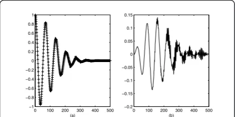
In this experiment, we create a 600 × 600 image which contains two concentric circles with radiusr01= 75 and r02 = 195; the center coordinates are {lc, mc} = {330, 315}, and the spread parameters ares1 = 9 ands2 = 9 (see Figure 9). The number of sensors of the circular antenna is set toS = 1500. The estimated parameters are as follows:

ˆ

r01= 75.4andr02ˆ = 195.0, the center coordinates are

ˆ

lc,mˆc

={330, 315}, and the spread parameters are ˆ

σ1= 9.1andσˆ2= 9.2.

Figure 10a shows the difference between the signal generated out of the image and the signal model created with the parameters which characterize the contours, and Figure 10b shows the difference between the signal generated out of the image superimposed with the signal generated with the estimated parameter values. The

relative error between the theoretical and the generated signals is 1.3 × 10-2, and the relative error between the estimated and the generated signals is 2.2 × 10-5. The estimated signal is closer to the generated signal than the model signal. This means that the proposed optimi-zation method is effective; and that the slight bias on the estimated spread values may come from a digitiza-tion effect during signal generadigitiza-tion on the circular antenna. For instance, if a one-pixel wide circle is expected, two connected pixels of the circle can share either a side or a corner. Therefore, they are not always at the same distance from each other, and also not always at the same distance from the point which is considered as the center of the circle. In the case of a blurred circle, the same remark holds. Nevertheless, as shown by the relative error values and by Figure 10, the generated, model, and estimated signals remain rather close to each other even for a relatively small image. The estimation of the center coordinates requires 3.05 × 10-2s, the estimation of the two radius values by TLS-ESPRIT requires 9.6 × 10-3 s, the estimation of the spread values with the proposed optimization method requires 6.9 × 10-1 s. The total running time for the proposed method is then 7.3 × 10-1 s. The Chan and Vese method requires 21.5 s, which is 29 times more than for the proposed method. This elevated computa-tional load is due to the large size of the image. On the contrary, the computational load of the proposed method (to which the optimization method essentially contributes) grows as a function of the number of sen-sors of the circular antenna and not as a function of the number of pixels in the image.

(a)

100 200 300 400 500 600 100

200

300

400

500

600

(b)

100 200 300 400 500 600 100

200

300

400

500

600

(c)

100 200 300 400 500 600 100

200

300

400

500

600

(d)

100 200 300 400 500 600 100

200

300

400

500

600

Figure 9Concentric blurred circles: (a) Processed image; (b) center circle; (c) final result obtained with the proposed methods; (d) result obtained by Chan and Vese. Results obtained on an image containing two concentric blurred circles by the proposed method and comparative method Chan and Vese.

0 100 200 300 400 500 −0.08

−0.06 −0.04 −0.02 0 0.02 0.04 0.06 0.08

(a)

0 100 200 300 400 500 −0.06

−0.04 −0.02 0 0.02 0.04 0.06 0.08

(b)

7.2.5 Note about the influence of the accuracy of the successive estimations

As we notice in Equation 9 of Section 4.2, the signal generated on the circular antenna exhibits a linear phase variation. This model holds only if the center of the circular antenna is superimposed with the center of the expected circle. In the experiments performed in this section, the maximum bias on a center coordinate is one pixel and the radius estimation is correct. Some experiments have shown that when this bias is more than three pixels, the estimation of the radius is affected. However, the proposed method for center coordinates estimation is reliable and does not yield pixel bias of more than one pixel. Also, some other experiments per-formed on the image of Section 7.2.1, by fixing artifi-cially the radius value which is used while estimating the spread value, have shown that the bias on the spread value is larger than 1 pixel only if the bias on the radius value is two pixels or more in absolute value. So, a slight bias, which does not exceed one pixel, on the radius value, does dot degrade the accuracy of the estimation of the spread value.

7.3 Circle detection in a correlated noise environment

7.3.1 Hand-made images containing two concentric one-pixel wide circles and correlated noise

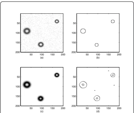
In this experiment, we create an image which contains two concentric circles with center coordinates {lc,mc} = {90, 95} and radius values 45 and 50 pixels, then per-form 100 trials with different correlated noise realiza-tions. We simulate correlated Gaussian noise by two steps: (1) generate random Gaussian noise matrix with amplitude in [0,1] and variance 1, which has the same size as the image; (2) let Gaussian noise matrix pass an isotropic spatial Gaussian low pass filter, whose filter

function is h(l,m) = 1 2πς2exp

−l2+m2

2ς2

. Besides, to

scale the degree of noise correlation, correlation length of generated Gaussian noise is defined asCL = 2ς. We set ςto 3.5. We expect to estimate the radius of multi-ple concentric circles by the proposed method based on higher-order statistics. An example of processed image is provided in Figure 11a.

When the proposed method is applied, MDL criterion is used to estimate the number of circles. The estimated radius values when the proposed method is used are, respectively, 44.5 and 51 pixels (see Figure 11b). The results of the proposed method are compared with those of the GHT [6]. GHT yields to estimated radius values 45.6 and 50.3 pixels (see Figure 11c). The visual aspect is the same for both methods. But the proposed method, the variant of TLS-ESPRIT which uses fourth-order cumulants, although being slower as the classical

TLS-ESPRIT (refer to the results above), is still five times faster than GHT method in the same experiment environment, respectively, 0.27 and 1.3 s.

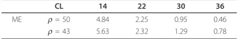
At the same time, we also analyze the effect of the correlation length of correlated noise. With the increase of correlation length of correlated noise, the grey level value of noise pixels decreases, but the noise correlation degree increases. The mean error on radius estimation is defined as ME= (1/N)N_i=1|ρ(i)−ρ|, where N = 100 is the number of trials andr(i) is the radius estima-tion at each trial. Table 3 shows that the mean error decreases when the correlation length of the correlated noise increases. That is because the correlated noise amplitude decreases.

In this section, we only considered one-pixel wide contours. Indeed, the GHT proposed in [6] is not meant for the estimation of a spread value. Future advances on the Hough transform could consist in deducing the spread parameter of blurred circles by measuring the peaks width of the relative maxima in the accumulator plane [6].

In the next section, we consider an image which con-tains both blurred circles and correlated noise.

(a) 50 100 150 200 20

40

60

80

100

120

140

160

180

200

(b) 50 100 150 200 20

40

60

80

100

120

140

160

180

200

(c) 50 100 150 200 20

40

60

80

100

120

140

160

180

200

Figure 11 Concentric circle retrieval in correlated noise environment: (a) Processed image with two concentric circles; (b) result obtained by the proposed method; (c) result obtained by GHT. Detection of two one pixel wide concentric circles in acorrelated noise environment.

Table 3 Mean errors (ME) vs correlation length (CL) (evolution of the mean error on the estimated radius values, respect to the noise correlation length)

CL 14 22 30 36

ME r= 50 4.84 2.25 0.95 0.46

7.3.2 Hand-made image containing two concentric blurred circles and correlated noise

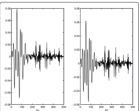
In this experiment, we create a 300 × 300 image which contains two concentric circles with radiusr01= 22 and r02= 90; the center coordinates are {lc,mc} = {135, 180}, and the spread parameters are s1 = 3 ands2 = 3. The image is artificially impaired with a correlated Gaussian noise with mean 0.1, standard deviation 0.1, and correla-tion length CL = 2. The estimated parameters are as follows:

ˆ

r01= 22 and r02ˆ = 91, the center coordinates are

ˆ

lc,mˆc

={135, 180}, and the spread parameters are ˆ

σ1= 3.9andσˆ2= 3.5.

Figure 12 shows that the center circles are correctly retrieved by the proposed methods, as well as the spread parameters, which provides a result image with contours which have the expected aspect (see Figure 12c). The time required to estimate the center is 3.0 × 10-2s, the time required to estimate the radii is 0.08 s, and the time required to estimate the spread values is 1.1 × 10-1 s. So the total computational load required by the pro-posed method is 2.2 × 10-1 s. The Chan and Vese method (see Figure 12d) requires 7.7 s. It is 35 times slower than the proposed method and does not provide information about the grey level variation around the center contour, only the inner and outer boundaries of the expected contours. This comparative method is then slower and provides less information as the proposed method.

7.4 Real-world image: influence of the Dove prism on a light beam

In this experiment, we consider two images which are a measurement of spatial light intensity. We aim at study-ing the effect of the Dove prism on the width of an opti-cal beam. Dove prisms are being extensively used in many physical settings that make use of the orbital angular momentum (OAM) of light (see [28] and refer-ences therein). The use of Dove prisms with highly focused beams requires some correcting elements whose characteristics can be determined though the influence of the Dove prism.

Figures 13 and 14 show two typical spatial shape mea-surements from light beams, the Dove prism being removed (Figure 13) or present (Figure 14). The beams which are presented are supposed to be highly focused. The experiment that we propose aims at checking that the Dove prism reduces the radius and spread of the light beam when the beam is highly focused. We also aim at calculating in what extent the characteristics of the beam are modified.

The estimated parameters are presented in Table 4. The results obtained presented in Table 4, in Figures 13d and 14d, show that Figure 13d contains the wide beam obtained without the Dove prism, and Figure 14d contains the straight beam obtained with the Dove prism.

As shown in Table 4, Figure 14 contains a beam with a radius which is 33% and a spread which is 27% smaller as the beam in Figure 13. We deduce from these blind

(a)

50 100 150 200 250 300 50

100

150

200

250

300

(b)

50 100 150 200 250 300 50

100

150

200

250

300

(c)

50 100 150 200 250 300 50

100

150

200

250

300

(d)

50 100 150 200 250 300 50

100

150

200

250

300

Figure 12Blurred circles in a correlated noise environment: (a) Processed image; (b) superposition processed image and center circle; (c) final result obtained with the proposed methods; (d) result obtained by Chan and Vese. Retrieval of two concentric blurred circles in a correlated noise environment.

(a)

50 100 150 200 250 300 50

100

150

200

250

300

(b)

50 100 150 200 250 300 50

100

150

200

250

300

(c)

50 100 150 200 250 300 50

100

150

200

250

300

(d)

50 100 150 200 250 300 50

100

150

200

250

300

measurements that the image of Figure 14 was obtained with a Dove prism.

Computing blindly the radius and spread of a light beam without and with Dove prism permits to evaluate the influence of this prism. As a consequence, the ade-quate compensating schemes, such as appropriate com-binations of cylindrical lenses [28], can be chosen and used to compensate for the Dove prism. A conclusion about the proposed methods and their performance is proposed in the following section.

8 Conclusion

The retrieval of blurred circle which may be concentric is considered in this article. To solve this issue, we pro-pose a model for the expected contours, which are char-acterized by four parameters of interest: the two circle coordinates, the radius, and the spread. We derive the model which fits the signals generated out of the image upon a circular antenna. This permits, after estimating the center by a linear antenna, to estimate the radius of

the expected circles. For this, when the noise is uncorre-lated, we adapt the TLS-ESPRIT method, a frequency retrieval method based on second-order statistics; when the noise is correlated, we adapt a novel version of TLS-ESPRIT, which is based on higher-order statistics, and faces correlated Gaussian noise. Then, we estimate the spread values by minimizing a least squares criterion between generated and model signals. For this, we adapt an ALS process which takes into account, while estimat-ing one spread value, the estimates of all other spread values. The proposed methods are successfully applied to various representative hand-made images. The results obtained are compared with those of Chan and Vese level set approach and GHT. The main advantage of the proposed methods is that not only the mean position of a contour is retrieved, but also the spread parameter which characterizes the gray level variations aside the contour mean position. Also, the proposed methods exhibit a lower computational load.

Some prospect for this study concerns the observed digitization effect. A more elaborated post-processing of the generated signal could be added. Also, we could alter the signal generation process to take into account this effect. Beyond the frame of this study, a possible advance could consist in a new version of the Hough transform, which may provide the spread value of circu-lar contours, through the width of the peaks of the accumulator plane of the Hough transform.

9 Annexe: Approximation of a Riemann summation as an integral

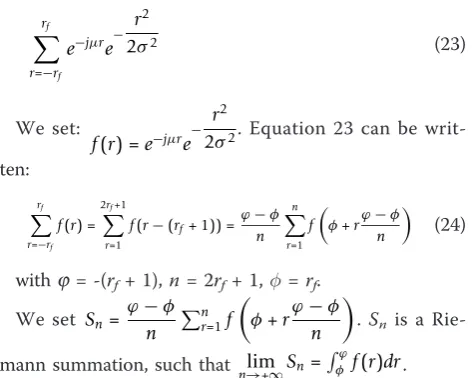
This annexe presents the validity of the approximation of a Riemann discrete summation as an integral. Let us consider the following expression:

rf

r=−rf

e−jμre− r2

2σ2 ₍₂₃₎

We set:

f(r) =e−jμr_e−

r2

2σ2. Equation 23 can be writ-ten:

rf

r=−rf f(r) =

2rf+1

r=1

f(r−(rf+ 1)) =ϕ−φ

n n

r=1 f

φ+rϕ−φ n

(24)

withj= -(rf+ 1),n= 2rf+ 1,=rf.

We set Sn= ϕ−φ

n

n

r=1f

φ+rϕ−φ n

. Sn is a

Rie-mann summation, such that lim

n→+∞Sn= _ϕ

φ f(r)dr. So, if we consider that rf is large enough, we get the following approximation:

(a)

50 100 150 200 250 300 50

100

150

200

250

300

(b)

50 100 150 200 250 300 50

100

150

200

250

300

(c)

50 100 150 200 250 300 50

100

150

200

250

300

(d)

50 100 150 200 250 300 50

100

150

200

250

300

Figure 14Beam obtained with a Dove prism: (a) color image; (b) processed image; (c) superposition processed image and center circle; (d) final result obtained with the proposed methods. Quantification of the influence of a Dove prism on the light beam coming from an optical system: beam obtained with a Dove prism.

Table 4 Estimated blurred circle parameters associated with Figures13 and 14 (the proposed method

characterizes the two blurred circles of Figures13 and 14 through their estimated center coordinates, radius, and spread)

Center Radius Spread

(a) {149; 154} 52.7 12.2

rf

r=−rf

f(r) = rf

−rf−1

f(r)dr (25)

Moreover, we notice that, ifsis small enough, |f(r)| decreases rapidly and is negligible for |r| >rf. Therefore, we can adopt the following approximation:

rf

−rf−1

f(r)dr

_∞

−∞f(r)dr (26)

So, from Equations 24 to 26, we get

rf

r=−rf

e−jμre− r2

2σ2

_∞

−∞e −jμr_e−

r2

2σ2_{dr (27)}

A general formula provides the equality

+∞

r=−∞

e−ar2+jbrdr=

π ae

−b

2

4a (28)

which yields

rf

r=−rf

e−jμre− r2

2σ2 √_2πσe−

μ2_σ2

2 (29)

which provides the expected approximation.

Competing interests

The authors declare that they have no competing interests.

Received: 3 July 2011 Accepted: 23 November 2011 Published: 23 November 2011

References

1. TF Chan, LA Vese, Active contours without edges. IEEE Trans Image Process.

10(2), 266–277 (2001). doi:10.1109/83.902291

2. L Benyoussef, C Carincotte, S Derrode, Extension of higher-order HMC modeling with application to image segmentation. Digital Signal Process.

18(5), 849–860 (2008). doi:10.1016/j.dsp.2007.10.010

3. RM Haralick, K Shanmugam, I Dinstein, Textural features for image classification. IEEE Trans Syst Man Cybern.3(6), 610_–621 (1973) 4. SMR Dehak, I Bloch, H Maitre, Spatial reasoning with incomplete

information on relative positioning. IEEE Trans Pattern Anal Mach Intell.

27(9), 1473–1484 (2005)

5. I Bloch, Fuzzy relative position between objects in image processing: a morphological approach. IEEE Trans Pattern Anal Mach Intell.21(7), 657–664 (1999). doi:10.1109/34.777378

6. DH Ballard, Generalizing the Hough transform to detect arbitrary shapes. Pattern Recogn.13(2), 111–122 (1981). doi:10.1016/0031-3203(81)90009-1 7. N Ayache, OD Faugeras, HYPER: a new approach for the recognition and positionning of two-dimensionnal objects. IEEE-PAMI8(1), 44–54 (1986) 8. J Borkowski, BJ Matuszewski, J Mroczka, LK Shark, Geometric matching of

circular features by least-squares fitting. Pattern Recogn Lett.23, 885–894 (2001)

9. JA Sethian,Level Set Methods and Fast Marching Methods, (Cambridge University Press, New York, 1999)

10. C Gout, C Le Guyader, L Vese, Segmentation under geometrical conditions using geodesic active contours and interpolation using level set methods. Numer Algor.39(1_–3), 155_–173 (2005). doi:10.1007/s11075-004-3627-8

11. E Erdem, S Tari, L Vese, Segmentation using the edge strength function as a shape prior within a local deformation model, inProceedings of ICIP, Cairo, 2989–2992 (October 2009)

12. S Krinidis, V Chatzis, Fuzzy energy-based active contours. IEEE Trans Image Process.18(12), 2747–2755 (2009)

13. R Arshizadeh, MM Ebadzadeh, Fuzzy external force for snake, inProceedings of ITNG, 2010, 376–381 (2010)

14. RO Schmidt, Multiple emitter location and signal parameters estimation. IEEE Trans Acoust Speech Signal Process.4(3), 276–280 (1983) 15. R Roy, T Kailath, ESPRIT, estimation of signal parameters via rotational

invariance techniques. IEEE Trans Acoust Speech Signal Process.37(7), 984–995 (1989). doi:10.1109/29.32276

16. HK Aghajan, T Kailath, Sensor array processing techniques for super resolution multi-line-fitting and straight edge detection. IEEE IP2(4), 454_–465 (1993)

17. HK Aghajan, Subspace techniques for image understanding and computer vision,PhD dissertation, Stanford University, Stanford, CA (1995)

18. J Marot, S Bourennane, Subspace-based and DIRECT algorithms for distorted circular contour estimation. IEEE Trans Image Process.16(9), 2369–2378 (2007)

19. J Marot, S Bourennane, Array processing for intersecting circle retrieval, in

Proceedings of EUSIPCO, August 2008, Lausanne), 5 (2009)

20. WP Krijnen, Convergence of the sequence of parameters generated by ALS algorithms. Comput Stat Data Anal.51(2), 481_–489 (2006). doi:10.1016/j. csda.2005.09.003

21. S Bourennane, J Marot, Contour estimation by array processing methods. Appl Signal Process. article ID 95634,15(2006). (2006)

22. S Bourennane, J Marot, Estimation of straight line offsets by a high-resolution method. IEE Vis Image Signal Process.153(2), 224–229 (2006). doi:10.1049/ip-vis:20050149

23. J Marot, S Bourennane, Propagator method for an application to contour estimation. Pattern Recogn Lett.28(12), 1556–1562 (2007). doi:10.1016/j. patrec.2007.03.013

24. S Bourennane, C Fossati, J Marot, Contour estimation in image using virtual signal. Opt Eng.49, 057002 (2010). doi:10.1117/1.3421576

25. M Wax, T Kailath, Detection of signals by information theoretic criteria. IEEE Trans Acoust Speech Signal Process.33(2), 387_–392 (1985). doi:10.1109/ TASSP.1985.1164557

26. N Yuan, B Friedlander, DOA estimation in multipath: an approach using fourth-order cumulants. IEEE Trans Signal Process.45(5), 1253–1263 (1997). doi:10.1109/78.575698

27. J Mendel, Tutorial on higher-order statistics (spectra) in signal processing and system theory: theoretical results and some applications. Proc IEEE.79, 278_–305 (1991). doi:10.1109/5.75086

28. N Gonzalez, G Molina-Terriza, JP Torres, How a Dove prism transforms the OAM of a light beam. Opt Express14(20), 9093_–9102 (2006). doi:10.1364/ OE.14.009093

doi:10.1186/1687-6180-2011-112

Cite this article as:Jianget al.:Circular contour retrieval in real-world conditions by higher order statistics and an alternating-least squares algorithm.EURASIP Journal on Advances in Signal Processing20112011:112.

Submit your manuscript to a

journal and benefi t from:

7Convenient online submission

7Rigorous peer review

7Immediate publication on acceptance

7Open access: articles freely available online

7High visibility within the fi eld

7Retaining the copyright to your article