Spatial-Temporal Clustering of Neural Data Using Linked-Mixtures of Hidden Markov Models

Volume 2009, Article ID 892461,16pages doi:10.1155/2009/892461

Research Article

Spatial-Temporal Clustering of Neural Data Using

Linked-Mixtures of Hidden Markov Models

Shalom Darmanjian and Jose Principe

Department of Electrical and Computer Engineering, University of Florida, Gainesville, FL 32611-6200, USA

Correspondence should be addressed to Shalom Darmanjian,oxygen@cnel.ufl.eduand Jose Principe,principe@cnel.ufl.edu

Received 1 February 2009; Revised 1 September 2009; Accepted 19 November 2009

Recommended by Don Johnson

This paper builds upon the previous Brain Machine Interface (BMI) signal processing models that require apriori knowledge about the patient’s arm kinematics. Specifically, we propose an unsupervised hierarchical clustering model that attempts to discover both the interdependencies between neural channels and the self-organized clusters represented in the spatial-temporal neural data. Results from both synthetic data generated with a realistic neural model and real BMI data are used to quantify the performance of the proposed methodology. Since BMIs must work with disabled patients who lack arm kinematic information, the clustering work described within this paper is relevant for future BMIs.

Copyright © 2009 S. Darmanjian and J. Principe. This is an open access article distributed under the Creative Commons Attribution License, which permits unrestricted use, distribution, and reproduction in any medium, provided the original work is properly cited.

1. Introduction

Unfortunately, thousands of people have suffered tragic accidents or debilitating diseases that have either partially or fully removed their ability to effectively interact in the external world. Some devices exist to aid these types of patients, but often lack the requirements to live a normal life. Essentially the idea behind motor Brain Machine Interfaces (BMIs) is to bridge the gap between the brain and the external world so that these patients can achieve effective interaction.

Generally, a BMI is a system that directly retrieves neuronal firing patterns from dozens to hundreds of neurons in the brain and then translates this information into desired actions in the external world. In particular, neural data is recorded from one or more cortices using one or multiple electrode grid arrays [1]. The amplified analog voltages recorded from one or more neurons are then digitally converted and passed to a spike sorting algorithm. Finally, the discrete binned spike counts are fed into to a signal processing algorithm [1] and subsequent trajectory/lever predictions are sent to robot arm or display device. All of the processing occurs as an animal engages in a behavioral experiment (lever press, food grasping, finger tracing, or joystick control).

Prior work showed that partitioning the neural input with a switching classifier improves trajectory reconstruction over conventional BMI feed-forward algorithms. Indirectly, the improvement provided evidence that the neural activity in the motor cortex transitions through multiple specific states during movement [2, 3] and that this switching behavior is exploitable for BMIs.

Unfortunately, to partition the neural input space, apri-ori class labels are needed for separation. However, under real conditions with paraplegics, there are no kinematic clues to separate the neural input into class labels (or clusters). Currently, most of the behaving animals engaged in BMI experiments are not paralyzed, allowing the kinematic information to be used in the training on the models. This Achilles heel plagues most BMI algorithms since they require kinematic training data to find a mapping to the neural data.

neural data without kinematic clues (i.e., unsupervised). In this paper, the Linked-Mixtures of Hidden Markov Models (LMs-HMMs) are combined with a clustering methodology in order to cluster neural data. The LM-HMM model is chosen since it operates solely in the input space and can characterize the temporal spatial space with a reduced computational cost. The methodology described in the next section will explain how the model learns the parameters and structure of the neural data in order to provide a final set of class or cluster labels for segmentation.

2. Generative Model and Clustering Framework

2.1. Related Work. The modeling approaches to BMIs are divided into three categories, supervised, coadaptive, and unsupervised, with the majority of BMI modeling algorithms being supervised. Additionally, most of the supervised algorithms further split into linear modeling, non-linear modeling, and state-space (or generative) modeling, with the majority of BMI algorithms falling under supervised linear modeling.

Supervised linear modeling is traceable to the 1980’s and 1990’s when neural action potential recordings were taking place with multi-electrode arrays [1, 5,6]. Essentially, the action potentials (called spikes for short), collected with microelectrode arrays, are sorted by neuron and counted in time windows (called bins) and fed into a linear model (Wiener filter) with a predefined tap delay line depending on the experiment and experimenter [7,8]. During training the linear model has access to the desired kinematic data, as a desired response, along with the neural data recording. Once a functional mapping is learned between the neural and kinematic training set, a test set containing only neural data is used on a linear model for reconstructing the kinematic trajectory [7].

The Wiener filter is exploited in two ways. First, it serves as a baseline linear classifier to compare results with the models discussed. Second, Wiener filters are used to reconstruct the trajectories from neural data switched by the generative models (see Figure 1). By comparing reconstructions from Wiener filters using our methodology, a reasonable metric can be established for unsupervised clustering in the absence of ground truths. Since the Wiener filter is critical to the paper and serves at the core of many BMI systems today, the details of the Wiener filter are presented in the appendix.

Along with the supervised linear modeling, researchers have also engaged in non-linear supervised learning algo-rithms for BMIs [1,8]. Very similar to the paradigm of the linear modeling, the neural data and kinematic data are fed to a non-linear model that finds the relationship between the desired kinematic data and the neural data. Then during testing only neural data is provided to predict kinematic reconstruction.

With respect to state-space models, Kalman filters have been used to reconstruct the trajectory of a behaving monkey’s hand [9, 10]. Specifically, they use a generative model for encoding the kinematic state of the hand. For

decoding, the algorithm predicts the state estimates of the hand and then updates this estimate with new neural data to produce a posteriori state estimate. Our group at UF and elsewhere found that the reconstruction was slightly smoother than what input-output models were able to produce [9,10].

Unfortunately, these supervised BMI models pose many problems. As mentioned, training with desired data is problematic since paralyzed patients cannot provide kine-matic data. Second, these models will not capture inhibited neurons, which are known to exist in the brain, since a neuron that fires very little will receive less weighting. Third, there are millions of other neurons not being recorded or accounted for in these models. Including that the missing information into the model would be beneficial. Lastly, all of the BMI models must generalize over a wide range of movements. Normally, generalization is good for a model of the same task, but generalization across tasks produces poor results.

The lack of a desired signal therefore necessitates the need for an unsupervised or coadaptive solution. Recent coadaptive solutions have relied on the test subject to train its brain for goal oriented tasks. Other researchers have used technicians to supply an artificial desired signal as the input-output models learn a functional mapping [11]. Sanchez et al. who used reinforcement learning coadapt their model and the rat’s behavior for goal-oriented tasks [12].

Other generative models (even graphical models like Hidden Markov Models—HMMs) [13–15] work on BMIs exploit the hidden state variables to decode possible states taken or transitioned by the behaving animal. Specifically, Kemere et al. found that HMMs can provide representations of movement preparation and execution in the hidden state sequences [15]. Unfortunately, this work also requires the use of supervision or a training data that must first be divided by human intervention (i.e., a user).

Although there is little BMI research into clustering neural data with graphical models, there have been efforts to use HMMs for clustering. The use of hidden Markov models for clustering appears to have first been mentioned in Juang and Rabiner [16] and subsequently used in the context of discovering subfamilies of protein sequences in Cadez and Smyth [17]. Other work use single HMM chains for under-standing the transition matrices [17]. The work described in this paper moves significantly beyond prior work since the clustering model finds unsupervised hierarchal dependencies between HMM chains (per neuron) while also clustering the neural data. Essentially the algorithm jointly refines the model parameters and structures as the clustering iterations occur. The hope is that the clustering methodology will serve as a front end for a goal-oriented BMI (with the clusters representing a specific goal, like “forward”) or for a coadaptive algorithm that needs reliable clustering of the neural input (seeFigure 1).

Preprocessing spike detection/sorting

Feed-forward models computing trajectory

Switching classifier selects corresponding forward model

Acquire multichannel neural data

O1 1

O1 2

O1

T O2

T

O2 1

O2 2

S2 1

S2 2

S2

T

S1

T

T1

T2

S1 1

S1 2

M1 _M2

· · ·

· · · ··· ···

Ti m

e

Neural channels Trajectory

reconstruction

Goal oriented actions or coadaptive algorithm

Figure1: BMI system overview.

hidden neural information is accomplished with observable and hidden random processes that are interacting with each other in some unknown way. To achieve this, we make the assumption that each neuron’s output is an observable ran-dom process that is affected by hidden information. Since the experiment does not provide detailed biological information about the interactions between the sampled neurons, we use hidden variables to model these hidden interactions [6,18]. We further assume that the compositional representation of the interacting processes occurs through space and time (i.e., between neurons at different times). Graphical models are the best way to model and observe this interaction between variables in space and time [19]. Another benefit of a state-space generative model over traditional filters is that neurons that fire less during certain movements can be modeled simply as another state rather than a low filter weight value.

Given the need to incorporate spatial dependencies between neural channels (which are known to be important) [20], Linked-Mixture of Hidden Markov Models (LM-HMMs) provides a way to help cluster the class labels while also clustering spatial dependencies between chan-nels.

Let Z represent the set of variables (both hidden and observed) included in the probabilistic model. A graphical model (or Bayesian network) representation provides insight into the probability distributions overZencoded in a graph structure [19]. With this type of representation, edges of the graph represent direct dependencies between variables. Conversely, and more importantly, the absence of an edge allows for the assumption of conditional independence

O1

1

O12

O1

T O2T

O2

1

O22

Q2

1

Q22

QT2

Q1T

T1

T2

Q1

1

Q12

M1 _M2

· · ·

· · ·

··· ···

Ti m

e

Neural channels Figure2: LM-HMM graphical model.

between variables. Ultimately, these conditional independen-cies allow a more complicated multivariate distribution to be decomposed (or factorized) into simple and tractable distributions [19].

Given the model parameters for a given HMM chainΘ= {A,B,π}, the log probability for this structure (Figure 2) is

logP(O,Q,M|Θ)

=logPM1₊

N

i=2

logPMi_|Mi−1_,Θi

+

N

i=1

⎛

⎝T

t=1

logPOit|Qti,Θi

+

T

t=1

logPQit|Qti−1,Mi,Θi

⎞

⎠_,

(1)

where the dependency between the tree cliques are repre-sented by a hidden variable Mi _{(corresponding to the ith}

neuron) in the second layer

PMi|Mi−1,Θi, (2) and the hidden stateQalso has a dependency on the hidden variableMin the second layer

PQti|Qti−1,Mi,Θi

. (3)

The lower observable variablesOi _{(shown inFigure 2)}

are conditionally independent from the second hidden layer variable Mi_{, as well as the sub-graphs of the other neural}

channels Tj _{(wherei /=j). The variables O}i _{are the actual}

bin counts observed from the ith neuron through time. The hidden variable M in the second layer of (2) can be interpreted as a mixture variable (when excluding the hierarchic links).

The LM-HMM is a compromise between making an independence assumption and a full dependence assump-tion. For further understanding and EM implementations please see the appendix and [20]. Although this hierar-chical model can find dependencies between channels in an unsupervised way, we still need to address how to obtain the class (or clustering) labels without user interven-tion.

2.3. Clustering Framework. This section establishes a model-based method for clustering the spatial-temporal neural signals using the LM-HMM. In effect, the clustering method tries to discover a natural grouping of the exemplar S

(i.e., window of multidimensional data or sequences of the neurons) into K clusters. A discriminate (distance) metric similar to K-means is used except that the vector centroids are now probabilistic models (LM-HMMs) representing dynamic temporal data [21].

The bipartite graph view (Figure 3) assumes a set of N data objects D (e.g., exemplars, represented by

S1,S2,. . .,SN), and K probabilistic generative models (e.g.,

HMMs), λ1,λ2,. . .,λK, each corresponding to a cluster of

exemplars (i.e., windows of data) [22]. The bipartite graph is formed by connections between the data and model spaces. The model space usually contains members of a

λ1

λ2

λK

. . .

. . .

Λ D

S1

S2

S3

SN

Figure3: Bipartite graph of exemplars (x) and models.

specific family of probabilistic models. A model λy can be

viewed as the generalized “centroid” of cluster y, though it typically provides a much richer description of the cluster than a centroid in the data space. A connection between an object S and a model λy indicates that the object S

is being associated with cluster y, with the connection weight (closeness) between them given by the log-likelihood logp(S|λy).

A straightforward design of a model-based clustering algorithm is to iteratively retrain models and repartition data objects. This can be achieved by applying the EM algorithm to iteratively compute the (hidden) cluster identities of data exemplars in the E-step and estimate the model parameters in the M-step. Although the model parameters start out as poor estimates, eventually the parameters hover around their true values as the iterations progress. The log-likelihoods are a natural way to provide distances between models as opposed to clustering in the parameter space (which is unknown). Basically, during each round, each training exemplar is re-labeled by the winning model with the final outcome retaining a set of labels that relate to a particular cluster or neural state structure (i.e., neural assembly) for which spatial dependencies have also been learned.

Setting the parameters can be daunting since the exper-imenter must choose the number of states, the length of the exemplar (window size) and the distance metric. To alleviate some of these model initialization problems, previous parameter settings found during early work are used for these experiments [4]. Specifically, an a-priori assumption is made that the neural channels are of the same window size and same number of hidden states. The clustering framework is outlined below.

Let data set D consist of N sequences for J neural channels,D = S11,. . .,SJN, whereS

j

n = (On₁j,. . .,On_{T j}) is a

sequences of observables lengthT andΛ = (λ1,. . .,λK) a

set of Models. We will refer to the multiple sequences in a window of time (sizeT) as an exemplar. The goal is to locally maximize the log-likelihood function:

logP(D|Λ)=

Sij∈D

logPSnj |λ_y(Sj n)

(1) Randomly assignKlabels (withK < N), one for each windowed exemplarSn, 1≤n ≤N. The LM-HMM

parameters are initialized randomly.

(2) Train each assigned model with the respective exem-plars using the LM-HMM procedure discussed in the appendix a and [20]. During this step the model learns the dependency structure for the current cluster of exemplars.

(3) For each model, evaluate the log-likelihood of each of theNexemplars given modelλi, that is, calculate Lin =log L(Sn | λi), 1 ≤ n ≤ N and 1 ≤ i ≤ K. y(Sn)= argmaxylogL(Sn|λi) is the cluster identity

of the exemplar. Then re-label all the exemplars based on cluster identity to maximize (4).

(4) Repeat steps (2) and (3) until convergence occurs or until a percentage of labeled exemplars does not change (i.e., set a threshold for changing exemplars). More advanced metrics for deciding when to stop cluster could be used (like KL divergence etc.).

3. Simulations

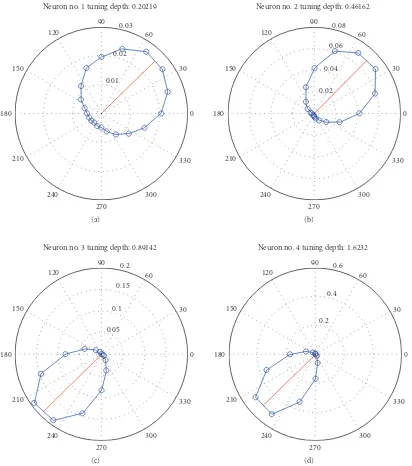
3.1. Simulated Data Generation. Since there are no ground truths to label real BMI neural data, simulations on plau-sible artificial data will help support the results found by the clustering framework on real data. Neurophysiologic knowledge provides an avenue to create a realistic BMI simulation since there is some evidence to suggest that neurons encode the direction of hand movements with cosine shaped tuning curves [5, 23]. These tuning curves provide a reference of activity for different neurons. In turn, this neural activity potentially relates to a kinematic vector, such as hand position, hand velocity, or hand acceleration, often using a direction or angle between 0 and 360 degrees. A discrete number of bins are chosen to coarsely classify all the movement directions. For the polar plots in this paper we chose 20 bins that each account for 18 degrees of the 360 degree space. For each direction, the average neural firing rate is obtained by using a non-overlapping window of 100 ms. Subsequently this average firing rate on the polar plot indicates the direction of velocities, and the magnitude of the vector is the average firing rate, marked as a blue circle, for each direction. The preferred direction is computed using circular statistics as

circular mean=arg

⎛

⎝

N rNeiΘN

⎞

⎠_{, (5)}

whererNis the neuron’s average firing rate for angleΘN, and Ncovers all the angle range.Figure 4shows the polar plot of four simulated neurons and the average tuning information with standard deviation across 100 Monte Carlo trials evaluated for 16 minutes duration. The computed circular mean, estimated as the firing rate weighted direction, is shown as a solid red line on the polar plot. The figure clearly indicates that the different neurons fired more frequently toward the preferred direction. Additionally, in order to get the statistical evaluation between Monte Carlo runs, the

traditional tuning depth were not normalized to (0, 1) for each realization as normally done in real data. To calculate the tuning depth:

Tuning Depth=max(rN)−min(rN)

std(rN) . (6)

A neural model must be selected in order to generate realistic simulated neurons. Although multiple models have been proposed [24, 25], we select the Linear-Nonlinear-Poisson (LNP) model since we can change different tuning properties to generate more realistic neural data. The LNP model consists of three stages. The first is a linear transformation that is then fed into a static non-linearity to provide the conditional firing rate for a Poisson spike generating model at the third stage [24,25].

Two simulated neural data sets are generated in the following experiments. One data set contains four neurons tuned to two classes (Figure 4) and a second data set contains eight neurons tuned to four classes. We first generate a velocity time series with 100 Hz sampling frequency and 16 minutes duration (1000000 samples totally). Specifically, a simple 2.5 kHz cosine and sine function are used to emulate the kinematics (X-Y Velocities) for the simulation experiments. For both data sets the entire velocity time series is passed through a (LNP) model with the assumed nonlinear tuning function in (7):

λt=exp

μ+βvtDprefer

, (7)

where λt is the instantaneous firing probability, μ is the

background firing rate (set to .00001). The variable β

represents the modulation factor for a preferred direction which we set monotonically from 1 to 4 for the four neurons in the two class simulation and a value of 3 for the eight neurons in the four class simulation. The unit vectorDprefer

is the preferred angular direction of the kinematics which we set to π/4 and 5π/4 for the two class simulation and

π/4, 3π/4, 5π/4, 7π/4 for the four class simulation (each direction is assigned two neurons for both simulations). The spike train is generated by an inhomogeneous Poisson spike generator using a Bernoulli random variable with probability

λ(t)Δtwithin each 1 ms time window. Once the spike trains

are generated, we bin them into 100 ms bins and down sample the velocityvtdata accordingly.

For each data set, an additional 100 randomly distributed spike trains (also 16 minutes each) are combined with the two data sets to create an artificial neural data set with a total of 104 and 108 neurons. Essentially, this allows for less than an 8% chance for the desirable channels to be randomly selected by the LM-HMMs.

0 30 60

90 120

150

180

210

240

270

300

330 0.01

0.02 0.03 Neuron no. 1 tuning depth: 0.20219

(a)

0 30 60

90 120

150

180

210

240

270

300

330 0.02

0.04 0.06

0.08 Neuron no. 2 tuning depth: 0.46162

(b)

0 30 60

90 120

150

180

210

240

270

300

330 0.05

0.1 0.15

0.2 Neuron no. 3 tuning depth: 0.89142

(c)

0 30 60

90 120

150

180

210

240

270

300

330 0.2

0.4 0.6 Neuron no. 4 tuning depth: 1.6232

(d) Figure4: Neural Tuning depth of four simulated neurons.

As seen from the figure, the model is able to correctly cluster the data in a relatively small number of iterations (three to four). For the first iteration, each exemplar in the full data set is randomly assigned to one of the clusters (indicated by green and blue colors). For the remaining iterations, a pattern starts to emerge that looks similar to the alternating kinematics. Although the kinematics (cosine and sine wave) are shown below the class labels, the clustering results were acquired solely from the input space.

Figure 6 shows the class tuning preference when the

model is initialized with random data. The term class tuning refers to the angular preference of the particular class (or cluster) label. It is calculated the same way as in neural tuning, except that the data is collected from the samples

that have been labeled by a particular class (i.e., circular statistics are calculated on the kinematics from class 3 rather than a neuron). Figure 7 shows the angular preference of the classes after clustering. Overlaid in blue is the original angular tunings of some of the neurons. We see that the model is able to successfully find the separation in neural firings.

1 2 3 4 5 6

It

er

ations

K

inematics

6150 6200 6250 6300

Time (100 ms bins) Random labels (uniform)

Figure5: LM-HMM cluster iterations (Two classes,k=2).

final result demonstrates that the clustering model with the LM-HMM is able to discover the underlying clusters present in the simulated neural data. Figure 9shows the clustering on the initial random labels whileFigure 10shows the tuned preference of the four classes after clustering. Remarkably it is able to determine the separation from the four classes using the neural input only. Next, the clustering model is tested for robustness when the number of clusters is unknown or increased noise is added to the neural data.

As with all clustering algorithms, choosing the correct number of underlying clusters is difficult. Choosing the number of clusters for BMI data is even more difficult since there are no known or established ground truths (with respect to motion primitives). To see the effect of defining too many clusters for the model,Figure 11illustrates when the clustering model is initialized with four classes (k = 4) despite the simulation only containing two underlying classes (or clusters) for the input space. Again, the results are gen-erated within a relatively small number of iterations. Notice from the figure that the extra two class labels are absorbed into the two classes shown in the previous Figure 5 (also shown below the four class labels). Interestingly, a repeated pattern of consistent switching occurs with the class labels (as indicated by the pattern of color blocks). Specifically,

Figure 11 shows that class 1 precedes class 3 and class 2, when combined, they correspond to class 1 inFigure 5, while class 4 inFigure 11corresponds to class 2 inFigure 5. This overlapping of clusters is common in clustering methods when the labels outnumber the true underlying number of classes [26]. Even the neural data from such a simple simulation is complicated yet remarkably the clustering method finds the consistent pattern of switching (perhaps indicating that the simple classes for further divisible).

For the final simulation, random spikes are added to the unbinned spiked trains of the earlier tuned neurons (Figure 4). Specifically, uniformly random spikes are gen-erated with a probability of spiking every 1 ms. Figure 12

shows the classification performance as the probability of

firing is increased from a 1% chance of spiking to 16% chance of spiking in 1 ms. Interestingly, the classification decreases but not significantly. The robustness is due to the tuned neurons still maintaining their underlying temporal structure.Figure 13shows the tuning polar plots of the four original neurons with the added random spikes. Although this figure shows that tuning seems to broaden across many angular bins, the random spikes do not have a temporal structure. Therefore they do not displace the temporal structure of the tuned neurons significantly (as indicated by only a small change in performance). Please note that increasing the probability of random spikes to 16% every 1 ms puts the spiking beyond the realistic firing rate of real neurons.

As a final note, the different artificial neurons are mod-ulated so that their tuning depth monotonically increased (i.e.,βset from 1 to 4). The LM-HMM clustering successfully selects the neurons in the correct order (respective to tuning depth) from the 100 random neural channels. The result is the same when the tuned neurons are corrupted with random spike noise.

4. Experimental Animal Data

4.1. Animal Data Collection. The animal data for these experiments were collected in the primate laboratory at Duke University. Using micro wire electrode arrays chronically implanted in the dorsal premotor cortex (PMd), supple-mentary motor area (SMA), primary motor cortex (M1, both hemispheres) and primary somatosensory cortex (S1), the firing times of up to 185 cells were simultaneously collected in an adult female monkey (Macaca mulatta) while performing a manipulandum behavioral tasks (cursor control) [1,27]. The monkey used a hand-held manipulan-dum (joystick) to move the cursor (smaller circle) so that it intersects the target. Upon intersecting the target with the cursor, the monkey received a juice reward. While the monkey performed the motor task, the hand position and velocity for each coordinate direction were recorded in real time along with the corresponding neural activity.Figure 14

illustrates that the majority of the monkey’s movement occurs diagonally.

In the second experiment, neural data was recorded from an owl monkey’s cortex as it performed a food reaching task. Specifically, multiple implanted micro-wire arrays recorded this data from 104 neural cells in the following cortical areas: posterior parietal cortex (PP), left and right primary motor cortex (M1), and dorsal premotor cortex (PMd). Concurrently with the neural data recording, the 3D hand position was recorded as the monkey made three repeated movements: rest to food, food to mouth, and mouth-to-rest [1,28].

0 30 60

90 120

150

180

210

240

270

300

330 0.2

0.4 0.6 Tuned preference before clustering

(a)

0 30 60

90 120

150

180

210

240

270

300

330 0.2

0.4 0.6 Tuned preference before clustering

(b) Figure6: Tuning Preference for two classes (initialized).

0 30 60

90 120

150

180

210

240

270

300

330 0.01

0.02 0.03

Tuned preference after clustering (versus tuned neurons)

(a)

0 30 60

90 120

150

180

210

240

270

300

330 0.05

0.1 0.15

0.2

Tuned preference after clustering (versus tuned neurons)

(b) Figure7: Tuned classes after clustering (two classes).

corresponds to a dataset of 26000×185 time bins. The time recording for the 3D food grasping monkey experiment corresponds to a dataset of 23000×104 time bins.

4.2. Experimental Results

4.2.1.2D Monkey Cursor Control. Two important questions must be answered with the following experiments. First, what type of clustering results are obtained, that is, are there repeating patterns corresponding to the kinemat-ics. Second, how does the trajectory reconstruction from the unsupervised clustering compare against the trajectory

reconstruction from supervised BMI algorithms. Classifica-tion performance is not considered in these experiments since there are no known classes by which to test. Although angular bins might serve the purpose for single neurons, the literature in this area is hotly contested. Therefore, correlation coefficient will serve as the metric and allow a consistent comparison between the results in this paper and previous work.

1 2 3 4 5 6 7

It

er

ations

K

inematics

3400 3450 3500 3550 3600 3650 3700 Time (100 ms bins)

Error Repeating pattern

Figure8: LM-HMM cluster iterations (Four classes,k=4).

(1) observation exemplar length (i.e., window size), (2) number of states,

(3) number of clustering rounds, (4) number of classes.

To determine the parameters, the observation length (window size) was varied from 5 to 15 time bins (corre-sponding to.5 seconds to 1.5 seconds). The number of hidden states was varied from 3 to 5. While the number of clustering iterations varied from 4 to 10. After exhausting the number of possible combinations, the parameters were set to: an observation length equal to 5 time bins, 3 hidden states and 6 clustering iterations (since less than 5% of the labels changed). These parameters are set the same for each neural channel.

The model was initialized with four classes after an empirical search (using different parameter sets). Since ground truths are unknown, trajectory reconstruction serves as the basis for how many clusters to select. Specifically, if reconstruction improves or diminishes then an adjustment to the number of clusters is made. Qualitatively,Figure 15

shows the labeling results from the LM-HMM clustering. TheY-Axis represents the number of iterations from random labels, to the final clustering iteration. Each color in the clustering results corresponds to a different class (four in all). The kinematics (x and y velocities) are overplayed at the bottom of the image for this cursor control experiment.

Figure 15 shows repetitive labeling for similar kinematic

profiles. These repetitive class transitions were also observed in the simulated data. Figure 16 shows trajectory recon-struction matches very closely to the original trajectory thereby indirectly validating the segmentation produced by the clustering method.

For a quantitative understanding, the correlation coef-ficient (CC) is a way to show if the clustering results have merit. Interestingly, the CC results for this unsupervised clustering are slightly better than the supervised echo state network and Wiener filter (Table 1). As expected random

Table1: Correlation coefficient using LM-HMM on 2D monkey data.

Experiment CC(X) CC(Y)

LM-HMM (unsupervised) .80 .69

LM-HMM (supervised) .82 .83

Echo State (supervised) .64 .78

NMCLM (FIR) .67 .50

NMCLM (Gamma) .67 .47

NLMS .68 .50

Gamma .70 .53

Subspace .70 .58

Weight Decay .71 .57

Kalman .71 .58

TDNN .65 .51

RMLP .66 .46

Random Labels .71 .67

labeling of the classes produces poor results compared to actual clustering. Additionally the random labeling results are similar to other supervised BMI models. As discussed earlier the similar results are due to the random clusters providing generalization of the full space for each filter (thereby becoming equivalent to a single Wiener filter).

Table 1shows that the correlation coefficient produced by the unsupervised LM-HMM clustering is slightly less than the correlation coefficient produced with the supervised version of the LM-HMM. This result is understandable since the supervised version of the LM-HMM can consistently isolate the neural data based on kinematic clues therefore improve reconstruction.

4.2.2. 3D Monkey Food Grasping Task. In this section, the LM-HMM is used to cluster the 3D monkey food grasping task. As with the cursor control experiment, Wiener filters are selected based on the class labels in order reconstruct the trajectory. This trajectory reconstruction is then compared to the supervised reconstruction. Qualitatively, Figure 17, shows that there is a corresponding clustering pattern to the kinematics. Although there areas of error or perceived errors (since there are no ground truths) since the most obvious kinematic feature (movement) is sometime missed in the figure.

Table 2 shows that the correlation coefficient on the

unsupervised LM-HMM clustering reconstruction is better than using random labeling or a single Wiener filter. Although the unsupervised results are not as good as the supervised version of the LM-HMM, it is remarkable that the unsupervised clustering can still outperform the majority of supervised BMI algorithms. This serves to validate that the segmentation is successful.

5. Discussion

0 30 60

90 120

150

180

210

240

270

300

330 0.1

0.2 0.3 Neuron no. 1 tuning depth: 0.1966

(a)

0 30 60

90 120

150

180

210

240

270

300

330 0.1

0.2 0.3 Neuron no. 2 tuning depth: 0.22704

(b)

0 30 60

90 120

150

180

210

240

270

300

330 0.1

0.2 0.3 Neuron no. 3 tuning depth: 0.21542

(c)

0 30 60

90 120

150

180

210

240

270

300

330 0.1

0.2 0.3 Neuron no. 4 tuning depth: 0.18902

(d) Figure9: Tuning Preference for four classes (initialized).

Table2: Correlation coefficient using LM-HMM on 3D monkey data.

Experiment CC

LM-HMM (unsupervised) .78

LM-HMM (supervised) .86

Single Wiener (supervised) .68

TDNN (supervised) .65

RMLP (supervised) .69

Kalman (supervised) .68

Random Labels .69

work to be done. This paper addressed one of the main problems associated with the signal processing side of BMIs

0 30 60

90 120

150

180

210

240

270

300

330 0.05

0.1 0.15

0.2 0.25 Tuning preference after clustering

(versus actual tuned neurons)

(a)

0 30 60

90 120

150

180

210

240

270

300

330 0.05

0.1 0.15

0.2 0.25 Tuning preference after clustering

(versus actual tuned neurons)

(b)

0 30 60

90 120

150

180

210

240

270

300

330 0.05

0.1 0.15

0.2 0.25 Tuning preference after clustering

(versus actual tuned neurons)

(c)

0 30 60

90 120

150

180

210

240

270

300

330 0.05

0.1 0.15

0.2 0.25 Tuning preference after clustering

(versus actual tuned neurons)

(d) Figure10: Tuned classes after clustering (four classes).

signal processing algorithms on real neural data. Although, trajectory reconstruction was used to show the validity of the clusters, the model could be used as front end for a co-adaptive algorithm or goal-oriented tasks (simple classifica-tion that paraplegics could select, i.e., move forward).

Despite these encouraging results, improvements in performance are possible for the hierarchical clustering. For example, the LM-HMM in the hierarchical clustering framework may not be taking full advantage of the dynamic spatial relationships. Specifically, spatial relationships may be evolving through time between the neurons. Although the hierarchical training methodology does create dependencies

between the HMM experts, perhaps there are better ways to exploit the dependencies or aggregate the local information. There may be important dependencies since different neural processes are interacting with other neural processes in an asynchronous fashion and that underlying structure could provide insight into the intrinsic communications occurring between neurons.

1 2 3 4 5

It

er

ations

K

inematics

1600 1650 1700 1750 1800

Time (100 ms bins) Random labels (uniform)

2-class LM-HMM labeling

Figure11: LM-HMM cluster iterations (Two classes,k=4).

to class 1. It would be interesting to investigate this further and see if perhaps there is a switching behavior between stationary points in the input space. Perhaps we can ascertain when a stationary switching point has occurred and exploit that information for modeling.

Appendix

A. LM-HMM Framework

A.1. LM-HMM Training with EM. We make approximations when finding the expectation of (1). In particular, we will first approximate P(Si

t | Sit−1,Mi,Θi) by treating Mi as

independent fromSmaking conditional probability equal to the familiarP(Si

t |Sit−1,Θi). Two important features can be

seen in this type of approximation. First we have decoupled the simple lower-level HMM chains from the higher-level

Mi _{variables. Second, M}i _{can now be regarded as a linked}

mixture variable for the HMM chains sinceP(Mi_|Mi−1_,Θi₎

which we will address later [29].

Because the lower-level HMMs have been decoupled, we are able to use the Baum-Welch formulation to compute some of the calculations in the E-step, leaving estimation of the variational parameter for later. As a result, we can calculate the forward pass.

E Step:

αj(t)=P

O1=o1,. . .,Ot=ot, St=j|Θ

. (A.1)

We can calculate this quantity recursively by setting

αj(1)=πjbj(o1),

αk(t+ 1)=

⎡

⎣N

j=1

αj(t)ajk

⎤

⎦_bk(ot+1). (A.2)

100 99 98 97 96 95 94

C

o

rr

ect

(r

elati

ve

to

init)

(%)

0 2 4 6 8 10 12 14 16 18

Firing in 1 ms (%)

Classification performance versus random firings

Figure 12: Classification degradation with increased random firings.

The well known backward procedure is similar:

βj(t)=P

Ot+1=ot+1,. . .,OT =oT |St=j,Θ

. (A.3)

This computes the probability of the ending partial sequence

ot+1,. . .,oTgiven the start at statejat timet. Recursively, we

can defineβj(t) as

βj(T)=1,

βj(t)= N

k=1

ajkbk(ot+1)βk(t+ 1).

(A.4)

Additionally, the ajk and bj(ot) matrices are the

tran-sition and emission matrices defined for the model which are updated in the M-step. Continuing in the E-step we will rearrange posteriors in terms of the forward and backward variables. Let

γj(t)=P

St=j|O,Θ

, (A.5)

which is the posterior distribution. We can rearrange the equations to quantities we have

PSt=j|O,Θ

= P

O,St= j|Θ

P(O|S,Θ)

= P

O,St=j|Θ

N

k=1P(O,St=k|Θ)

,

(A.6)

and now with the conditional independencies we can define the posterior in terms ofα’s andβ’s:

γj(t)=

αj(t)βj(t)

N

k=1αk(t)βk(t).

0 30 60

90 120

150

180

210

240

270

300

330 0.05

0.1 0.15

0.2 Neuron no. 1 tuning depth: 0.06057

(a)

0 30 60

90 120

150

180

210

240

270

300

330 0.05

0.1 0.15

0.2 0.25 Neuron no. 2 tuning depth: 0.1908

(b)

0 30 60

90 120

150

180

210

240

270

300

330 0.1

0.2 0.3

0.4 Neuron no. 3 tuning depth: 0.45368

(c)

0 30 60

90 120

150

180

210

240

270

300

330 0.2

0.4 0.6

0.8 Neuron no. 4 tuning depth: 1.0622

(d) Figure13: Neural Tuning depth with high random firing rate.

We also define

ξjk(t)=P

St=j,St+1=k|O,Θ

(A.8) which can be expanded:

ξjk(t)=P

St=j,St+1=k,O|Θ

P(O|S,Θ)

=N αj(t)ajkbk(ot+1)βk(t+ 1)

j=1

N

k=1αj(t)ajkbk(ot+1)βk(t+ 1) .

(A.9)

The M-step departs from the Baum-Welch formulation and introduces the variational parameter [30]. Specifically, the M-step involves the update of the parametersπj,ajk,bL

(we will saveuifor later)

M Step:

πi j=

I

i=1uiγ1i

j

I

i=1ui

,

aijk =

I

i=1ui

T−1

t=1 ξti

j,k

I

i=1ui

T−1

t=1 γti

j ,

bi j(L)=

I

i=1ui

T

t=1δot,vLγti

j

I

i=1ui

T−1

t=1 γit

j .

(A.10)

0.3 0.2 0.1 0

−0.1

−0.2

−0.3

−0.4

Y

ve

lo

ci

ti

es

−0.2 −0.15 −0.1 −0.05 0 0.05 0.1 0.15

Xvelocities

XversusYvelocities

Not unifor m accr

ossall angles

Figure14: 2D Angular Velocities.

0 2 4 6 8

It

er

ations

K

inematics

5900 5950 6000 6050 6100

Time (100 ms bins) Random labels (uniform)

Repeating patterns

Figure15: LM-HMM cluster iterations (Ivy 2D dataset,k=4).

0.05

0

−0.05

−0.1

Tr

aj

ec

to

ry

920 940 960 980 1000 1020 1040 1060 Time (100 ms)

Predicted and real trajectory

Figure16: Reconstruction using unsupervised LM-HMM clusters (blue) versus Real Trajectory (red).

2 4

6

Ite

ra

ti

o

n

s

K

inematics

6500 7000 7500 8000 8500 9000 9500 10000 Time (100 ms bins)

Random labels (uniform) DC-HMM clustering (2 classes)

Figure17: LM-HMM Clustering on monkey food grasping task (2 classes).

A.2. Updating Variational Parameter via Importance Sam-pling. While still working within the EM framework, we treat the variational parametersuias mixture variables generated

by theith HMM each having a prior probability of pi_{. We}

want to estimate the set of parameters that maximize the likelihood function [17,31,32]:

n

z=1

I

i=1

piPOzi|Si,Θi. (A.11)

Given the set of exemplars and current estimates of the parameters, the E-step consists of computing the conditional expectation of hidden variableM:

uzi=E

Mi_|Mi−1_,Ozi_|Θi

=PrMi=1|Mi−1_=1,Ozi_,Θi_.

(A.12)

The problem with this conditional expectation is the dependency onMi−1_{. SinceM}i−1_{is independent fromO}i_and

Θi_{we can decompose this into}

uzi=E

Mi|Ozi,ΘiEMi|Mi−1. (A.13)

The first term, a well-known expectation for Mixture of Experts, is calculated by using Bayes rule and the priori probability thatM=1:

EMi_|Oi_,Θi_=PrMi=1_|Oi_,Θi₌ piP

Oi_|Si_,Θi

I

i=1piP(Oi|Si,Θi)

the integration with a lower variance than Monte-Carlo integration [33]. We can approximate the integration with

EMi_|Mi−1₌ 1

n n

z=1

POzi_|Si_,Θi

P(Oz(i−1)_|Si−1_,Θi−1₎. (A.15)

where the n samples have been drawn from the proposal distributionP(Ozi−1 _{| S}i−1_{,Θ). For the estimation ofu}

iwe

need to combine the two terms:

uzi= p

i_POzi_|Si_,Θi

I

i=1piP(Ozi|Si,Θi)

n

z=1

POzi_|Si_,Θi nP(Oz(i−1)_|Si−1_,Θi−1₎.

(A.16) To compute the M-step,

pi=

n

z=1uzi

I

i=1

n

z=1uzi

=

n

z=1uzi

n . (A.17)

Borrowing from the competitive nature of the BM-HMM, we choose winners based on the same criterion of minimizing the Euclidean distance for the classes for the LM-HMM.

Acknowledgments

The authors thank Johan Wessberg and Miguel A. L. Nicolelis for sharing their monkey data and experience. They also thank Yiwen Wang for providing the code for the neural model used in their simulations. This paper was supported by DARPA project no. N66001-02-C-8022 and NSF project no. 0540304.

References

[1] M. A. L. Nicolelis, D. Dimitrov, J. M. Carmena, et al., “Chronic, multisite, multielectrode recordings in macaque monkeys,”Proceedings of the National Academy of Sciences of the United States of America, vol. 100, no. 19, pp. 11041–11046, 2003.

[2] E. Todorov, “On the role of primary motor cortex in arm movement control,” inProgress in Motor Control III, M. L. Latash and M. F. Levin, Eds., chapter 6, pp. 125–166, Human Kinetics, 2001.

[3] L. Goncalves, E. D. Bernardo, and P. Perona, “Movemes for modeling biological motion perception,” inSeeing, Thinking and Knowing, vol. 38 of Theory and Decision Library A, Springer, Dordrecht, The Netherlands, 2004.

[4] S. Darmanjian, S. P. Kim, M. C. Nechyba, et al., “Bimodal brain-machine interface for motor control of robotic pros-thetic,” inProceedings of the IEEE International Conference on Intelligent Robots and Systems, vol. 4, pp. 3612–3617, 2003. [5] A. P. Georgopoulos, J. T. Lurito, M. Petrides, A. B. Schwartz,

and J. T. Massey, “Mental rotation of the neuronal population vector,”Science, vol. 243, no. 4888, pp. 234–236, 1989. [6] A. B. Schwartz, D. M. Taylor, and S. I. H. Tillery, “Extraction

algorithms for cortical control of arm prosthetics,”Current Opinion in Neurobiology, vol. 11, no. 6, pp. 701–708, 2001. [7] S.-P. Kim, J. C. Sanchez, D. Erdogmus, et al.,

“Divide-and-conquer approach for brain machine interfaces: nonlinear mixture of competitive linear models,”Neural Networks, vol. 16, no. 5-6, pp. 865–871, 2003.

[8] J. C. Sanchez, S.-P. Kim, D. Erdogmus, et al., “Input-output mapping performance of linear and nonlinear models for estimating hand trajectories from cortical neuronal firing patterns,” in Proceedings of the International Workshop for Neural Network Signal Processing, pp. 139–148, 2002. [9] W. Wu, M. J. Black, Y. Gao, et al., “Neural decoding of

cursor motion using a Kalman filter,” inAdvances in Neural Information Processing Systems, vol. 15, pp. 133–140, MIT Press, Cambridge, Mass, USA, 2003.

[10] Z. Li, J. E. O’Doherty, T. L. Hanson, M. A. Lebedev, C. S. Henriquez, and M. A. L. Nicolelis, “Uscented Kalman lter for brain-machine interfaces,” PLoS ONE, vol. 4, no. 7, article e6243, 2009.

[11] L. R. Hochberg, M. D. Serruya, G. M. Friehs, et al., “Neuronal ensemble control of prosthetic devices by a human with tetraplegia,”Nature, vol. 442, no. 7099, pp. 164–171, 2006. [12] J. C. Sanchez, B. Mahmoudi, J. DiGiovanna, and J. C. Principe,

“Exploiting co-adaptation for the design of symbiotic neuro-prosthetic assistants,”Neural Networks, vol. 22, no. 3, pp. 305– 315, 2009, special issue on Goal-Directed Neural Systems. [13] G. Radons, J. D. Becker, B. Dulfer, and J. Kruger, “Analysis,

classification, and coding of multielectrode spike trains with hidden Markov models,”Biological Cybernetics, vol. 71, no. 4, pp. 359–373, 1994.

[14] I. Gat,Unsupervised learning of cell activities in the associative cortex of behaving monkeys, using hidden Markov models, M.S. thesis, Hebrew University, Jerusalem, Israel, 1994.

[15] C. Kemere, G. Santhanam, B. M. Yu, et al., “Detecting neural-state transitions using hidden Markov models for motor cortical prostheses,”Journal of Neurophysiology, vol. 100, no. 4, pp. 2441–2452, 2008.

[16] B. H. Juang and L. R. Rabiner, “Issues in using hidden Markov models for speech recognition,” inAdvances in Speech Signal Processing, S. Furui and M. M. Sondhi, Eds., pp. 509–553, Marcel Dekker, New York, NY, USA, 1992.

[17] I. Cadez and P. Smyth, “Probabilistic clustering using hierar-chical models,” Tech. Rep. 99-16, Department of Information and Computer Science University of California, Irvine, Calif, USA, 1999.

[18] W. J. Freeman,Mass Action in the Nervous System, University of California, Berkeley, Calif, USA, 1975.

[19] M. I. Jordan, Z. Ghahramani, and L. K. Saul, “Hidden Markov decision trees,” inAdvances in Neural Information Processing Systems, M. C. Mozer, M. I. Jordan, and T. Petsche, Eds., vol. 9, MIT Press, Cambridge, Mass, USA, 1997.

[20] S. Darmanjian and J. C. Principe, “Boosted and linked

mixtures of HMMs for brain-machine interfaces,”EURASIP

Journal on Advances in Signal Processing, vol. 2008, Article ID 216453, 12 pages, 2008.

[21] A. Y. Ng, M. I. Jordan, and Y. Weiss, “On spectral clustering: analysis and an algorithm,” inAdvances in Neural Information Processing Systems, T. G. Dietterich, S. Becker, and Z. Ghahra-mani, Eds., vol. 14, pp. 849–856, MIT Press, Cambridge, Mass, USA, 2002.

[22] S. Zhong and J. Ghosh, “A unified framework for model-based clustering,”Journal of Machine Learning Research, vol. 4, no. 6, pp. 1001–1037, 2004.

[23] A. P. Georgopoulos, J. F. Kalaska, R. Caminiti, and J. T. Massey, “On the relations between the direction of two-dimensional arm movements and cell discharge in primate motor cortex,”

[24] E. P. Simoncelli, L. Paninski, J. Pillow, and O. Schwartz, “Characterization of neural responses with stochastic stimuli,” inThe New Cognitive Neurosci, MIT Press, Cambridge, Mass, USA, 3rd edition, 2004.

[25] Y. Wang, J. C. Sanchez, and J. C. Principe, “Information theoretical estimators of tuning depth and time delay for motor cortex neurons,” inProceedings of the 3rd International IEEE/EMBS Conference on Neural Engineering, pp. 502–505, 2007.

[26] T. Lange, M. Braun, V. Roth, and J. M. Buhmann,

“Stability-based model selection,” to appear in Advances in Neural

Information Processing Systems.

[27] J. Wessberg, C. R. Stambaugh, J. D. Kralik, et al., “Real-time prediction of hand trajectory by ensembles of cortical neurons in primates,”Nature, vol. 408, no. 6810, pp. 361–365, 2000. [28] S. Darmanjian, S. P. Kim, M. C. Nechyba, et al., “Bimodal

brain-machine interface for motor control of robotic pros-thetic,”IEEE Machine Learning for Signal Processing, vol. 4, pp. 379–384, 2006.

[29] R. A. Jacobs, M. I. Jordan, S. J. Nowlan, and G. E. Hinton, “Adaptive mixtures of local experts,”Neural Computation, vol. 3, pp. 79–87, 1991.

[30] M. I. Jordan, Z. Ghahramani, T. S. Jaakkola, and L. K. Saul, “An introduction to variational methods for graphical models,” in

Learning in Graphical Models, MIT Press, Cambridge, Mass, USA, 1998.

[31] J. Alon, S. Sclaroff, G. Kollios, and V. Pavlovic, “Discovering clusters in motion time-series data computer vision and

pattern recognition,” in Proceedings of the IEEE Computer

Society Conference, vol. 1, pp. 375–381, 2003.

[32] A. Ypma and T. Heskes, “Categorization of web pages and user clustering with mixtures of hidden Markov models,” in

Proceedings of the International Workshop on Web Knowledge Discovery and Data Mining, pp. 31–43, Edmonton, Canada, 2002.