Volume 2008, Article ID 837102,12pages doi:10.1155/2008/837102
Research Article
Experimental Evaluation of Adaptive Modulation and
Coding in MIMO WiMAX with Limited Feedback
Christian Mehlf ¨uhrer, Sebastian Caban, and Markus Rupp
Institute of Communications and Radio-Frequency Engineering, Vienna University of Technology, Gusshausstrasse 25/389, 1040 Vienna, Austria
Correspondence should be addressed to Christian Mehlf¨uhrer,[email protected]
Received 22 June 2007; Revised 3 October 2007; Accepted 28 November 2007
Recommended by Ana P´erez-Neira
We evaluate the throughput performance of an OFDM WiMAX (IEEE 802.16-2004, Section 8.3) transmission system with adaptive modulation and coding (AMC) by outdoor measurements. The standard compliant AMC utilizes a 3-bit feedback for SISO and Alamouti coded MIMO transmissions. By applying a 6-bit feedback and spatial multiplexing with individual AMC on the two transmit antennas, the data throughput can be increased significantly for large SNR values. Our measurements show that at small SNR values, a single antenna transmission often outperforms an Alamouti transmission. We found that this effect is caused by the asymmetric behavior of the wireless channel and by poor channel knowledge in the two-transmit-antenna case. Our performance evaluation is based on a measurement campaign employing the Vienna MIMO testbed. The measurement scenarios include typical outdoor-to-indoor NLOS, outdoor-to-outdoor NLOS, as well as outdoor-to-indoor LOS connections. We found that in all these scenarios, the measured throughput is far from its achievable maximum; the loss is mainly caused by a too simple convolutional coding.
Copyright © 2008 Christian Mehlf¨uhrer et al. This is an open access article distributed under the Creative Commons Attribution License, which permits unrestricted use, distribution, and reproduction in any medium, provided the original work is properly cited.
1. INTRODUCTION
With the theoretical understanding of the nature of multiple antenna systems in a scattering environment by Winters [1], Foschini and Gans [2], and Telatar [3], an enormous potential for high spectral efficiency was found. This gave the motivation to include multiple antenna systems in wireless transmission standards like UMTS [4], WiMAX [5], and WLAN [6]. A summary of all these standardization efforts is given in [7]. They have in common that the amount of feedback information is limited to a few bits per transmission frame, preventing the implementation of optimal beamforming solutions [8–10] that allow for close-to-capacity performance.
In this work, we measure the throughput performance of a SISO/MIMO OFDM system that uses the coding and modulation schemes defined in the WiMAX standard IEEE 802.16-2004 [5, Section 8.3], and [11]. The feedback mechanism in WiMAX is limited to 3 bits by which one out of seven possible adaptive modulation and coding (AMC)
schemes is selected, for example, depending on the received SNR.
Multiple transmit antennas are incorporated into the WiMAX standard by Alamouti space-time coding [12] at the transmitter, thus increasing the available receive SNR and the spatial diversity. This allows to reuse the same feedback as in the SISO case for the Alamouti coded system. In addition to Alamouti space-time coding, we consider spatial multiplexing with individual AMC at every of the two transmit antennas as an extension to the WiMAX standard [13]. In particular, four different transmission modes were
implemented and measured.
(Mode 1) This mode is the standardized single transmit antenna system with 3-bit feedback.
(Mode 2) This is the standardized two-transmit-antenna system with Alamouti coding with also 3-bit feedback.
(equal coding rate at both antennas). This mode is incorporated in the following mode but its throughput is evaluated separately.
(Mode 4) This is a spatial multiplexing, two-transmit-antenna system using 6-bit feedback (individual coding rate at both antennas).
The measured data throughput of these transmission modes is compared to the mutual information of the wireless channel when the transmitter has no channel knowledge.
Previous work in this field is based either on simulations [14–16] or on channel sounding experiments that yield channel coefficients and channel capacities for different scenarios [17,18]. To the authors’ knowledge, no work exists so far where the data throughput of a MIMO WiMAX system is measured and compared to the mutual information of the channel. Such a comparison is of utmost importance to identify potential weaknesses of a transmission system and to propose possible enhancements.
The paper is organized as follows. Section 2 presents the transmitter and receiver algorithms used to generate the transmit signals and to evaluate the receive signals, respectively. Section 3provides an overview of the Vienna MIMO testbed and the setup of transmitter and receiver in our measurement scenarios. InSection 4, we introduce a so-called “perfect” AMC feedback method. Section 5includes a derivation of the achievable data throughput based on the mutual information of the channel. The measured data throughput is presented inSection 6. InSection 7, we draw our conclusions. In Appendix Awe substantiate our findings from the measurement results by simulating the system performance in a well-defined environment. Finally,
inAppendix Bthe SNR gains of improved channel estimators
are evaluated.
2. BASEBAND PROCESSING
In this section, the data generation at the transmitter and the data processing at the receiver are explained for the four different transmission modes considered in our experiments. Specifically, we distinguish between SISO/SIMO transmis-sion, MISO/MIMO transmission with Alamouti space-time coding, and MIMO transmission with spatial multiplexing. In the case of a single transmit antenna and for Alamouti mode, a single data stream is transmitted, while for spatial multiplexing, two independently coded and modulated data streams are transmitted.
2.1. Transmitter
At first, random data bits are generated and then coded by a concatenated Reed-Solomon (RS) and convolutional encoder (see Figure 1). The systematic outer RS code uses a codeword length of 255 bytes, a data length of 239 bytes, and a parity length of 16 bytes. Depending on the currently selected AMC value, the RS code is shortened (to allow for smaller block sizes) and punctured. The outer convolutional code of rateR=1/2 is generated by the polynomials 171OCT
and 133OCT. This code belongs to the class of the so-called
maximum free distance codes with constraint length seven. However, after puncturing depending on the AMC value, the maximum free distance is reduced todfree =6 forR=2/3,
dfree=5 forR=3/4, anddfree=4 forR=5/6, respectively,
dfree=10).
After coding, an interleaver is implemented to avoid long runs of low reliable bits at the decoder input. The interleaved bits are mapped adaptively to a symbol alphabet. The coding, interleaving, and symbol mapping are the same as defined in the WiMAX IEEE 802.16-2004 specification [5]. Depending on the feedback information from the receiver, the mapping and the coding rate are adjusted. The seven possibilities for the AMC schemes are summarized inTable 1. When Alamouti transmission is selected, the symbols are additionally space-time coded to generate the transmit symbols for both antennas. For spatial multiplexing, the SISO encoding and modulation mapping are used for both transmit antennas separately, leading to a total number of 7 ×7=49 AMC schemes.
After mapping the bits to symbols, serial-to-parallel conversion is carried out to form OFDM symbols (256 carrier OFDM with 192 data symbols). Pilots, training symbols, a zero DC carrier, and guard carriers are added as defined in [5]. After an inverse fast Fourier transfor-mation (IFFT), a cyclic prefix is added. We chose a cyclic prefix length of 1/4 of the total OFDM symbol length to avoid intersymbol interference in all measurement scenarios. Before transmitting over the wireless channel, the signal is normalized by a factor 1/NT(withNTcorresponding to the
number of transmit antennas), ensuring equal total signal power for single and multiple antenna transmissions. Note that base stations are subject to a power constraint by the telecommunications regulator. To satisfy such a constraint, we introduced the above normalization. Therefore, in SISO transmissions the single transmit antenna radiates twice the power of each (2 TX) MIMO antenna.
2.2. Receiver
Data bits RS
encoder Puncture
Convolutional
encoder Puncture
Symbol
mapping STC
AMC information from receiver
To OFDM modulator
Figure1: Encoding and modulation at the transmitter.
Table1: The WiMAX AMC schemes in our setup for single antenna and Alamouti transmission. For spatial multiplexing, a separate AMC scheme can be used for every transmit antenna. These frame sizes correspond to 44 OFDM data symbols transmitted in a frame duration of 2.5 milliseconds.
AMC scheme Data bits per frame Modulation Coding rate Max. throughput
(1) 4224 2-PAM 1/2 1.69 Mbps
(2) 8448 4-QAM 1/2 3.38 Mbps
(3) 12672 4-QAM 3/4 5.07 Mbps
(4) 16896 16-QAM 1/2 6.76 Mbps
(5) 25344 16-QAM 3/4 10.14 Mbps
(6) 33792 64-QAM 2/3 13.52 Mbps
(7) 38016 64-QAM 3/4 15.21 Mbps
all measurement results are based on least-squares channel estimation.
The channel estimates and the data symbols are passed to a max-log-MAP (maximum a posteriori) demapper. The demapper for the spatial multiplexing transmissions is implemented as a soft output sphere decoder with a single-tree search [20]. The resulting soft bits are passed to a Viterbi decoder and then to a Reed-Solomon decoder.
3. MEASUREMENTS
When it comes to measuring systems with feedback, there are basically three approaches.
(i) One might build a demonstrator [21] where the whole system (including the feedback) [22] is imple-mented in real-time.
(ii) One might use a testbed where the received data is evaluated “quickly” (e.g., in Matlab or C) and the feedback is carried out via a LAN-connection. In such a scenario, round trip times (receiver algorithm in Matlab + LAN + transmitter algorithm in Matlab + loading the data into the testbed) are usually in the order of 100 milliseconds up to a second, depending on the effort put into the implementation. This feedback method is especially interesting for indoor scenarios where the channel stays constant over such long periods of time, if carried out, for example, at night. In outdoor scenarios, trees, cars, and other constantly moving uninfluenceable objects may prohibit such a measurement.
(iii) One might not use feedback at all but transmit a block of data for every possible feedback combina-tion, to evaluate these blocks later on. Of course, this is only realizable in the case of limited feedback.
Approaches one and two require the knowledge of some method to select the AMC scheme. These two approaches are not applicable if the method of extracting the feedback bits from the received data is yet to be found. Also, only one particular feedback method can be investigated in one measurement. We therefore decided to implement the third approach, explained in detail in the following. This approach has the advantage that also an optimal feedback method can be investigated allowing to benchmark other realistic methods based on, for example, the received SNR.
3.1. Measurement setup
For our measurements, we utilize the Vienna MIMO testbed described in [23] enhanced by new power and low-noise amplifiers. The basic features of the testbed are as follows.
(i) Baseband processing is carried out offline in Matlab with floating-point precision. The transmitted and received down-sampled signals are stored on hard disk drives (approximately 600 Gbytes per scenario measured).
(ii) Receiver and transmitter are synchronized by means of rubidium frequency standards and a LAN connec-tion.
(iii) The carrier frequency is 2.5 GHz; the bandwidth is 5 MHz.
by 2.75λ). Reference measurements using the two different polarizations of only one antenna yielded the same conclusions and are therefore not further discussed in this paper.
(v) The receive antennas are placed on a stepper-motor-controlled linear XY positioning table. This table was placed at three positions resulting in the following three measurement scenarios.
(a) InScenario 1, the table was placed two floors below the transmit antenna in the same build-ing havbuild-ing a non-line-of-sight connection. (b) InScenario 2, the table was placed in a
non-line-of-sight connection in the courtyard next to the transmit antenna.
(c) A line-of-sight connection was established in
Scenario 3by placing the table with the receive
antennas in the adjacent building (Figure 2). These three practical scenarios represent three different locations of a user accessing the internet via a WiMAX connection.
3.2. Measuring a scenario
For each of the scenarios, we transmitted the following blocks of data (Figure 3).
(a) A 2.5-millisecond long block, encoded according to every possible feedback value (AMC value), was transmitted.
(b) Consecutively, 7 SISO blocks, 7 Alamouti coded blocks, and 7×7 blocks employing spatial multiplex-ing were transmitted.
(c) The resulting 7+7+7×7=63 blocks were transmitted at 15 different transmit power levels (28 dBm down to−2 dBm in steps of 2 dB) which was achieved by analog attenuation of the transmitted signal prior to the power amplifier.
(d) After reception, the resulting 15×(7+7+7×7) blocks were stored on hard disks for offline processing in Matlab. The mean performance of a specific sce-nario was obtained by repeating the above described transmission at 502 different positions of the receive antenna uniformly distributed within an area of 4λ× 4λ(corresponding to a distance of 0.18λbetween the measurement positions). Note that more positions within the same area would not significantly increase the accuracy of the results because the channel realizations become correlated. The only method to increase the number of realizations is to increase the measurement area, but this would lead to undesired large-scale fading effects.
3.3. Measured channels
The method of successively transmitting all AMC schemes requires that the channel stays constant during the trans-mission of the 63 blocks to obtain meaningful throughput
5
.
5
λ
2.75λ
TX
RX
1.2 λ
x-axis
Figure2: Transmit and receive antenna setups in the outdoor-to-indoor LOS scenario.
results. Large channel coherence time was achieved by performing the outdoor-to-indoor measurements in the late evening and by locking up the room with the receiver. The outdoor-to-outdoor measurements were also performed in a closed courtyard where no persons/objects moved around.
The time-invariance of the frequency response from transmit antenna one to receive antenna one is illustrated
in Figure 4. In this figure, the estimated channel
coeffi-cients of the successively transmitted data blocks (at the same overall transmit power level) are plotted on top of each other. The estimated channel coefficients include all amplification and attenuation factors (including transmit power normalization) applied to the signal after the training signal generation. These attenuation factors are thus part of the estimated channel. Because of the transmit power normalization, the frequency responses of the seven SISO AMC schemes are 3 dB larger than the frequency responses of the MIMO AMC schemes. It should be emphasized that the channel characteristics (gain and receiver noise variance) stay constant also for the transmission at different transmit power levels.
(a) AMC =1
AMC =2
AMC =3
· · ·
AMC =last
t
(b) SISO Alamout i
Spatialmultiple xing
7x 7x 49x
t
(c)
Tran smit powe
r =28
dBm
=26 dBm
=24 dBm
· · · =− 2 dBm
t
(d) Po
sitio n1
Posit ion
2
Posit ion
3
· · · Po sition
502
t
Save data to HDD
+ move antennas
Figure3: Structure of the transmitted data blocks, (a) is a zoomed version of (b).
−30 −20 −10 0 10 20 30
|
h1,1
|
2
σ
2n
(dB)
20 40 60 80 100 120 140 160 180 Sub carrier index
SISO
MIMO 3 dB
Figure 4: Estimated channel coefficients for the SISO as well as the MIMO cases between transmit antenna one and receive antenna one, scenario 1, NLOS outdoor-to-indoor. The coefficients are plotted over the 192 data subcarriers; the eight pilots and the zero DC carrier are left out. Note that the transmitter attenuation is included in these estimated channel coefficients leading to 3 dB smaller channel coefficients for MIMO transmis-sions.
Because of the above described reasons, we can consider the scenarios as quasistatic during all transmissions at a given receive antenna position.
4. BEST AMC SELECTION
We define the best possible AMC selection as the one that maximizes the data throughput. Since all AMC schemes are transmitted consecutively over approximately the same channel, we can evaluate all schemes and select the one that achieves the highest throughput. This perfect feedback scheme and the method of calculating the data throughput for this scheme will be explained in the following.
We calculate the data throughput for the following receiver schemes.
Single receive antenna schemes
(i) SISO transmission of a single data stream. The receiver
selects one of the seven AMC schemes shown inTable 1. This requires a 3-bit feedback for every frame.
(ii) 2×1MISO transmission of a single Alamouti
space-time coded data stream. The same AMC schemes as for the
SISO transmission are employed.
Dual receive antenna schemes
(i)SIMO transmission of a single data stream with maximum
ratio combining at the receiver. The same AMC schemes as for
the SISO transmission are employed.
(ii)MIMO transmission of a single Alamouti space-time
coded data stream with maximum ratio combining at the
receiver. Again, the same AMC schemes as for the SISO
transmission are employed.
(iii) 2×2MIMO transmission of two data streams. Both data streams are encoded by thesamemodulation and coding scheme. The feedback effort here is therefore the same as in the SIMO transmission, that is, 3 bits.
(iv) 2 × 2 MIMO transmission of two independent
data streams. Every data stream is encoded and modulated
as defined for the SISO transmission, leading to a total combination of 7 × 7 = 49 schemes with an overall feedback effort of 6 bits. Note that this mode includes all possible modulation and coding schemes of the previous transmission mode.
At a specific channel realizationc =1,. . .,NRXposand a
specific transmit attenuator valuem=1,. . ., 15, we calculate the best instantaneous data throughput as
D(bestc,m)=maxi∈I Ri
1−Pi(c,m)
, (1)
where Ri corresponds to the data rate of the ith adaptive
modulation and coding scheme (i ∈ I, whereIis the set of all adaptive schemes) andPi(c,m) ∈ {0, 1}is a frame error
channel realizations (NRXposreceiver positions) at a specific
attenuationm:
D(best,avgm) = 1 NRXpos
NRXpos
c=1
D(bestc,m). (2)
Note that (2) gives the absolute maximum data throughput that is possible with the available transmission schemes. This data rate can only be achieved by a genie-driven AMC selection that knows the block errors of all transmission schemes already before the actual transmission. In a real system, the selection of an appropriate AMC value would have to rely on the channel state information and the estimated noise variance to predict the block errors for all AMC schemes. The nontrivial problem of selecting the appropriate AMC value is not addressed in this work.
5. ACHIEVABLE DATA THROUGHPUT
In this section, we derive an expression for the “achievable” data throughput that can be used as a performance bound for the measured data throughput. This expression is based on the mutual information between transmit and receive signals, that is, the estimated frequency response. The achievable data throughput is only a function of the wireless channel and does not depend on the AMC schemes used in the measurements.
Consider the mutual information of an AWGN channel with the SNRρ:
I=log2{1 +ρ}, (3) In theory, a transmission can achieve a rate corresponding to this mutual information. This requires that the transmitter adapts the coding rate to the receive SNR. Therefore, the receiver has to feed back which AMC value the transmitter has to use. In WiMAX, seven AMC schemes corresponding to 3-bit feedback are defined.
The mutual information for transmitting symbols over a MIMO channel (which correspond to the mutual infor-mation of thekth subcarrier of the OFDM system) can be expressed as [2,3]
Ik(c,m)=log2
det
INR+
1 σ2
n
Hk(c,m)Hk(c,m)H . (4)
(In literature, the mutual information is often referred to as “capacity without channel knowledge at the transmitter.” However, the capacity is a property of the channel and cannot depend on the particular implementation of a transmission system (e.g., with or without full channel knowledge at the transmitter). We will therefore base the calculation of the achievable data throughput on the mutual information.) Equation (4) assumes that the transmitter has no knowledge about the channel, and thus the transmit power is distributed equally over the antennas. Using (4), we can estimate the theoretically achievable transmission rate by substituting the true channel matrix H(c,m) with the estimated channel
matrix H(estc,m). To improve the accuracy of the mutual
information, we use the channel matrices estimated by the
genie-driven channel estimator that utilizes all transmitted data symbols. Additionally, we calculate the channel matrices for large transmit attenuator values from the estimated channel matrix at the smallest transmit attenuator value
H(estc,m)=Am
A1H (c,1)
est , m=2,. . ., 15. (5)
Here,Amdenotes themth transmit attenuation value andA1
corresponds to the smallest attenuation. The noise variance σ2
n is also substituted by the estimated noise variance. It
is approximately the same at both receive antennas with a difference of about 1 dB.
The overall mutual information Isum(m) for the OFDM
system at one transmit attenuation value m can now be calculated by summing the mutual information of all subcarriers and averaging over theNRXpos (the realizations)
different receiver positions:
I(m) sum=
1 NRXpos
NRXpos
c=1 192
k=1
Ik(c,m). (6)
Since the transmission of an OFDM signal requires also the transmission of a cyclic prefix to avoid intersymbol interference, and a preamble for synchronization and chan-nel estimation, the mutual information given by (6) can never be achieved. It is therefore convenient to introduce an “achievable” data throughputDachievable(m) that accounts for
these inherent system losses. We define the achievable data throughput at the transmit attenuation valuemas
Dachievable(m) =
1 1 +G·
1/Ts
256· Ndata
NOFDM·I (m)
sum, (7)
where G (1/4 in our measurements) corresponds to the ratio of cyclic prefix time and useful OFDM symbol time, Ndata (44 in our measurements) is the number of OFDM
data symbols,NOFDM(47 in our measurements) is the total
number of OFDM symbols in one transmission frame, and Ts corresponds to the sampling rate of the transmit
signal. The factor (1/Ts)/256 is therefore equivalent to the
available bandwidth per subcarrier. In our measurements, we chose a channel bandwidth of 5 MHz. For this channel bandwidth, the WiMAX standard defines a sampling rate ofTs = 1/5.76 MHz. The 5.76 MHz total signal bandwidth
emerging from this sampling rate fits into the 5 MHz channel bandwidth because some of the guard band carriers (with zero energy) are outside the 5 MHz channel bandwidth.
Equation (7) will be used as a performance bound for comparisons with the measured data throughput in the next section.
6. RESULTS
0 5 10 15 20 25 30
Thr
o
ug
hput
(Mbit/s)
0 4 8 12 16 20 24 28
Transmit power (dBm) Achievable throughput
Single TX (1) Single TX (2)
Dual TX
1×1
2×1 Alamouti
Figure 5: Scenario 1, measured (solid) and achievable (dashed) data throughput in the NLOS outdoor-to-indoor scenario using one receive antenna. The largest transmit power corresponds to a receive SNR of about 22 dB.
6.1. Scenario 1—NLOS outdoor-to-indoor
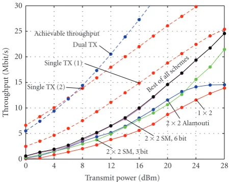
In this scenario, the receiver was placed three floors below the transmit antenna mounted on a pole on the roof, resulting in a non-line-of-sight outdoor-to-indoor connection. The scenario is characterized by strong frequency selectivity and hence large frequency diversity. The measured data throughput is shown for one and two receive antennas in Figures 5 and6, respectively. In Figure 5, we observe that the achievable data throughput is approximately the same for a two-transmit-antenna transmission and a transmission on the first transmit antenna only. The achievable data throughput of the second transmit antenna is a little bit lower than that of the first transmit antenna.
One would expect from simulation results that Alamouti transmission greatly outperforms SISO transmission in such a strong frequency selective scenario (seeAppendix A.2for a simulation result in an ITU Pedestrian B channel). The gain of the Alamouti transmission over the SISO transmission is caused by the ability to “flatten” the frequency response of the channel by utilizing the spatial diversity. This, in turn, increases the probability of correctly decoding the received frame. Unfortunately, Alamouti transmissions are more sensitive to channel estimation errors than SISO transmissions (see, e.g., the derivation of the bit error probability of a 2×1 Alamouti transmission and a 1×2 transmission with maximum ratio combining in [26]). This results in a loss of all performance gains of the Alamouti coded system, as shown in Figure 5. In addition to the higher sensitivity of the Alamouti transmission to channel estimation errors, also the channel estimator performance in the Alamouti case is worse than in the SISO case. The reason for this lies in the fact that in a two-antenna transmission the available transmit power is split between antennas causing the received training to be of 3 dB lower SNR. In this scenario, the performance of the Alamouti transmission can be enhanced by a better channel estimator.
0 5 10 15 20 25 30
Thr
o
ug
hput
(Mbit/s)
0 4 8 12 16 20 24 28
Transmit power (dBm) Achievable throughput
Single TX (1) Single TX (2)
Dual TX
1×2 2×2 Alamouti 2×2 SM, 6 bit
2×2 SM, 3 bit
Bestof allsch
emes
Figure 6: Scenario 1, measured (solid) and achievable (dashed) data throughput in the NLOS outdoor-to-indoor scenario using two receive antennas. The largest transmit power corresponds to a receive SNR of about 22 dB.
0 5 10 15 20 25 30
Thr
o
ug
hput
(Mbit/s)
−5 0 5 10 15 20
Estimated mean SNR (dB) Achievable throughput
Single TX (1) Dual TX
1×2 2×2 Alamouti
2×2 SM, 3 bit 2×2 SM, 6 bit
Best ofall
schem es
Figure 7: Scenario 1, measured (solid) and achievable (dashed) data throughput in the NLOS outdoor-to-indoor scenario using two receive antennas.
If, for example, LMMSE channel estimation is implemented, the Alamouti transmission could gain about 1.2 dB over the SISO transmission (see alsoTable 2inAppendix Bfor a list of channel estimation gains).
our case, this is achieved by changing the coding rate, but the same effect may also be achieved by Alamouti coding with a subsequent power loading on the transmit antennas. This, however, requires that both power amplifiers are capable of transmitting at the full output power of the SISO system (3 dB more than in the MIMO case).
The “best of all schemes” curve shows the data through-put if the best transmission scheme is selected from the set ofall possible AMC schemes at every receiver position (for every channel realization). This means that not only the AMC scheme is adapted to the channel but also the transmission mode, that is, single stream, Alamouti, or spatial multiplexing. In the low SNR region, the single stream transmission is selected most of the time; in the high SNR region, spatial multiplexing achieves the largest data throughput. Note that the “best of all schemes” throughput is sometimes larger than the throughput of the individual transmission modes. This is due to the individual selection of the transmission modes for every channel realization.
Figure 7 shows the throughput in the same scenario
plotted over receive SNR. The throughput for the 1×2 system here is equal to the throughput of the 2×2 Alamouti system. In contrast, when these curves are plotted over transmit power, the 1×2 system shows an advantage of about 1 dB over the Alamouti system. When comparing systems with a different number of transmit antennas (e.g., SISO with Alamouti), we encounter the fact that the two transmit antennas do not have the same average channel gain. If those systems are compared over receive SNR, the throughput curves are shifted and, therefore, the results look different. For this reason, we plot all curves over transmit power rather than over receive SNR.
6.2. Scenario 2—NLOS outdoor-to-outdoor
In this scenario, the receive antennas were placed in a non-line-of-sight connection in the courtyard next to the building with the transmit antennas on the roof. The results for this scenario with strong frequency selectivity are shown in Figures 8and9. In contrast to the previous scenario, a transmission over the second transmit antenna leads to a
muchhigher achievable throughput than a transmission over the first antenna. Therefore, adding the second antenna at the transmitter by Alamouti coding yields a significant through-put increase. On the other hand, if the SISO transmission had been performed over the second transmit antenna, Alamouti coding would have worsened the performance. We therefore conclude that in such a strongly asymmetric scenario, antenna selection is a promising alternative.
Figure 9 shows that the 2 × 2 transmission already
achieves such a large SNR that the data throughput for the single stream transmission saturates (since no larger AMC values are available). In this SNR region, the usage of spatial multiplexing yields a large throughput increase. Also, due to the strongly asymmetric scenario, the 6-bit spatial multiplexing system greatly benefits from the adjustable code rate per transmit antenna.
0 5 10 15 20 25 30
Thr
o
ug
hput
(Mbit/s)
0 4 8 12 16 20 24 28
Transmit power (dBm)
Achievable throughput Dual TX Single TX (1) Single TX (2)
1×1 2×1 Alamouti
Figure 8: Scenario 2, measured (solid) and achievable (dashed) data throughput in the NLOS outdoor-to-outdoor scenario using one receive antenna. The largest transmit power corresponds to a receive SNR of about 24 dB.
0 5 10 15 20 25 30
Thr
o
ug
hput
(Mbit/s)
0 4 8 12 16 20 24 28
Transmit power (dBm)
Achievable throughput Dual TX Single TX (1)
Single TX (2)
1×2 2×2 Alamouti 2×2 SM, 6 bit 2×2 SM, 3 bit
Best ofall
schemes
Figure 9: Scenario 2, measured (solid) and achievable (dashed) data throughput in the NLOS outdoor-to-outdoor scenario using two receive antennas. The largest transmit power corresponds to a receive SNR of about 24 dB.
6.3. Scenario 3—LOS outdoor-to-indoor
In this scenario, a line-of-sight connection was established by placing the receive antennas inside a building adjacent to the building with the transmit antennas on the roof. The measured data throughput is shown for one and two receive antennas in Figures10and11, respectively. This scenario is characterized by a strong line-of-sight component leading to Rician distributed flat fading channels. The RicianKfactor [27] was estimated to be K = 2.9. (The RicianK factor is defined as the relation between the energy of the nonfading line-of-site (specular) component and the energies of the diffuse fading components, K = s2/2σ2, given pdf(x) =
(x/σ2) exp−((x2+s2)/2σ2)I
0 5 10 15 20 25 30
Thr
o
ug
hput
(Mbit/s)
0 4 8 12 16 20 24 28
Transmit power (dBm) Achievable throughput
Dual TX
Single TX (1) Single TX (2)
1×1
2×1 Alamouti
Figure10: Scenario 3, measured (solid) and achievable (dashed) data throughput in the LOS outdoor-to-indoor scenario using one receive antenna. The largest transmit power corresponds to a receive SNR of about 32 dB.
0 5 10 15 20 25 30
Thr
o
ug
hput
(Mbit/s)
0 4 8 12 16 20 24 28
Transmit power (dBm)
Achievable throughput Dual TX Single TX (1) Single TX (2)
1×2
2×2 Alamouti 2×2 SM, 6 bit
2×2 SM, 3 bit
Best ofall
schemes
Figure11: Scenario 3, measured (solid) and achievable (dashed) data throughput in the LOS outdoor-to-indoor scenario using two receive antennas. The largest transmit power corresponds to a receive SNR of about 32 dB.
The Alamouti code looses a lot of performance compared to the transmission with a single antenna. Here, in contrast to the previous two scenarios, the loss is caused by the flat fading channel (see Appendix Afor simulation results). It is well known that in flat fading channels, the diversity can be increased by Alamouti coding. At a fixed modulation and coding scheme, the Alamouti coded system therefore has an increasing SNR advantage for large SNR values. However, since we are considering a coded system with adaptive modulation and coding, the operating points on the uncoded BER curves are between BER=10−1 and BER=10−2. At
these large BER values, the SNR gain due to Alamouti coding is only very small [28, pages 777–795] and vanishes
when coded frame error rate or data throughput is plotted.
Appendix A shows a simulation result for a flat fading
Rice scenario (similar to the measured one) where the same effect can be observed. Additionally, Alamouti coding looses because of the poor channel estimation, as discussed above.
The 2×2 spatial multiplexing system suffers in this scenario from the line-of-sight component. For low transmit power, the performance is worse than the 1 × 2 per-formance. However, for large transmit power (>16 dBm), the throughput of the single stream transmission already saturates allowing for huge performance gains of the spatial multiplexing schemes. In such a scenario with a line-of-sight connection to the basestation, either new AMC values with larger data rate or spatial multiplexing should be implemented.
6.4. Discussion of the throughput loss
The measured throughput curves presented in the previous sections have in common that they are far (>10 dB) away from the achievable throughput. We identified the following factors as the main sources of the SNR loss.
(i) The largest loss is caused by the too simple convolu-tional channel coding which shows a relatively slow decline of the coded BER curve. The slow decline of the coded BER curve also leads to poor frame error ratio (FER) performance for large block lengths. (The frame error probability Pf for a frame ofNf bits
can be calculated from the bit error probabilityPbas
Pf =1−(1−Pb)Nf.) As shown inAppendix A, the
convolutional coding already costs >6.5 dB in SNR for a SISO transmission over a flat Rayleigh fading channel. Our preliminary assessments show that this loss can be decreased greatly if better channel codes (LDPC or Turbo codes) are employed.
7. CONCLUSIONS
In this paper, we investigated the throughput performance of SISO and MIMO WiMAX systems with limited feedback. Our evaluation is based on an extensive outdoor measure-ment campaign using practical setups of the basestation antennas and receiver positions. The comparison of the mea-sured data throughput to the “achievable” data throughput, given by the mutual information of the channel, reveals a large loss (>10 dB in SNR). Even the single transmit antenna schemes only achieve a fraction of the possible data throughput. The largest part of this SNR/throughput loss is caused by the simple convolutional coding (about 6.5 dB). By using improved coding techniques (LDPC or Turbo codes), it should be possible to reduce this loss greatly. Another significant part of the SNR/throughput loss is caused by simple LS channel estimation. Depending on the transmission scheme, this loss is between 0.6 dB and 3.2 dB. The implementation of a WiMAX system therefore requires improved channel coding (e.g., the optional block Turbo code of the WiMAX standard) and enhanced channel estimators.
The comparisons between the different schemes revealed that Alamouti and spatial multiplexing transmissions (3-bit feedback) loose performance compared to SIMO and spatial multiplexing (6-bit feedback) transmissions. This is caused by the asymmetric gains of the MIMO chan-nel. Therefore, also asymmetric transmission schemes are required to achieve high performance. Asymmetric trans-mission on two antennas can be accomplished by spatial multiplexing with individual coding and modulation for each transmit antenna, as investigated in the paper. Other possibilities may be, for example, transmit antenna selection or Alamouti transmission with subsequent power loading on the two transmit antennas. This, however, would require that both transmit amplifiers support the full transmit power of the SISO amplifiers (3 dB more than the MIMO amplifiers).
A very general conclusion of this work is that the overall performance of a communication system obviously depends on several factors. If a single part of a system is not implemented properly (e.g., channel coding, channel estimation), the overall system performance is substantially reduced. Only a thorough investigation comparing measured throughput to achievable throughput (given by the mutual information of the wireless channel) reveals whether all parts of a wireless system are properly configured. In the special case of WiMAX 802.16-2004, our performance analysis reveals that the optional channel coding schemes should be implemented before the optional MIMO extensions since advanced channel coding promises substantially larger gains.
APPENDICES
A. SIMULATIONS
In this appendix, we present some additional results confirm-ing the statements inSection 6.
0 2 4 6 8 10 12 14 16
Thr
o
ug
hput
(Mbit/s)
−5 0 5 10 15 20
SNR (dB)
Achievable throughput
∼8 dB
∼5.5 dB
AMC7 AMC6
AMC5
AMC4 AMC3 AMC2 AMC1
Figure12: Simulated throughput performance of the SISO system with perfect channel knowledge in an AWGN channel.
0 2 4 6 8 10 12 14 16
Thr
o
ug
hput
(Mbit/s)
−5 0 5 10 15 20 25 30 35 SNR (dB)
Achievable throughput
∼8 dB
∼6.5 dB
Simulated throughput
Figure13: Simulated throughput performance of the SISO system with perfect channel knowledge in a flat Rayleigh fading channel.
A.1. SISO performance
In this section, we investigate the performance loss of the simple convolutional coding and the limited number of AMC schemes. As can be observed in the AWGN simulations
inFigure 12, the loss to the achievable throughput is about
0 2 4 6 8 10 12 14 16 18 20
Thr
o
ug
hput
(Mbit/s)
0 5 10 15 20 25 30
SNR (dB) 2×1 Alamouti perfect CSI
1×1 perfect CSI
1×1 estimated CSI
2×1 Alamouti estimated CSI
Figure 14: Simulated throughput performance for perfect and estimated channels, Pedestrian B channel model without spatial correlation.
A.2. SNR loss due to channel estimation
A.2.1. Frequency selective channel
The first comparison (Figure 14) shows the simulated data throughput of the one receive antenna system in an ITU Pedestrian B [29] environment. No correlation was assumed between the transmit antennas. The figure shows the throughput for estimated and perfectly known channels. When perfect channel state information (CSI) is available at the receiver, the Alamouti transmission has superior performance over the SISO transmission throughout the entire SNR range. When the channel is estimated at the receiver, the Alamouti transmission looses about 2.4 dB in SNR, much more than the SISO (0.8 dB) leading to only slightly better performance of the Alamouti transmission in the high SNR region. One reason for the poor channel knowledge in the two-transmit-antenna case is the power splitting on the two transmit antennas. This leads to the reception of the training with 3 dB smaller SNR and, hence, a worse channel estimate than in the SISO case (see also
Figure 4). Another reason for the poor channel estimate
lies in the fact that the WiMAX standard defines only one OFDM training symbol per transmit antenna not allowing for an enhanced channel estimator that makes use of several training symbols.
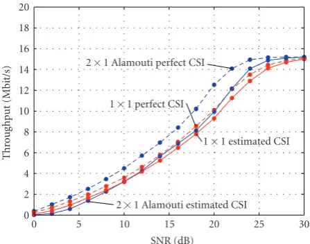
A.2.2. Flat fading LOS scenario
In this simulation, we compare the throughput performance of 2×1 Alamouti transmission to the 1×1 SISO transmission in a flat fading Rice channel withK = 2.9. The results are plotted inFigure 15. When perfect channel state information is available at the receiver, the 2×1 and 1 ×1 systems show the same performance; only at a large SNR, Alamouti coded transmission has a small advantage. Since the system operates at a high uncoded BER, the diversity gain of the Alamouti code is not reflected in the data throughput. Note
0 2 4 6 8 10 12 14 16 18 20
Thr
o
ug
hput
(Mbit/s)
0 5 10 15 20 25 30
SNR (dB) 2×1 Alamouti perfect CSI
1×1 perfect CSI
1×1 estimated CSI 2×1 Alamouti estimated CSI
Figure 15: Simulated throughput performance for perfect and estimated channels, flat fading Rice channel withK=2.9.
Table2: SNR gains of improved channel estimators over the LS estimator.
Scenario 1 LMMSE genie-driven
1×1 SISO 0.6 dB 1.2 dB
2×1 Alamouti 1.8 dB 2.9 dB
1×2 SIMO 0.5 dB 1.2 dB
2×2 Alamouti 1.9 dB 3.2 dB
2×2 Spatial Multiplexing (3 bit) 1.4 dB 2.4 dB 2×2 Spatial Multiplexing (6 bit) 1.1 dB 2.2 dB
the difference to the previous simulation in the Pedestrian B environment where Alamouti has a 2 dB gain over the SISO transmission. In the frequency selective case, the Alamouti code “flattens” the frequency response and thus avoids deep fades (that would inhibit the correct decoding of the received frame) of some subcarriers. Therefore, space-time coding has the ability to increase the data throughput in frequency selective channels and not in flat fading channels.
B. SNR GAINS OF IMPROVED CHANNEL ESTIMATORS
To quantify the SNR loss of the simple least-squares chan-nel estimator, the received data were also evaluated with improved channel estimators. In particular, LMMSE channel estimation and genie-driven channel estimation were con-sidered. The genie-driven estimator uses all transmitted data symbols (44 OFDM symbols) to obtain a channel estimate.
Table 2 shows the SNR gains of these improved channel
estimators over the least-squares estimator for measurement scenario one. In scenarios 2 and 3, the SNR gains of the improved channel estimators are approximately the same. A difference of only±0.2 dB was observed [30].
ACKNOWLEDGMENTS
Raschko, Robert Langwieser, Michael Fischer, and Werner Keim. Without their valuable contributions to the testbed, these measurements could not have been performed. The authors would also like to thank Professor Kathrein for providing the basestation antennas for their measurement campaign. This work has been funded by the Christian Doppler Laboratory for Design Methodology of Signal Pro-cessing Algorithms (seehttp://www.nt.tuwien.ac.at/cdlab/).
REFERENCES
[1] J. H. Winters, “On the capacity of radio communication systems with diversity in a rayleigh fading environment,”IEEE Journal on Selected Areas in Communications, vol. 5, no. 5, pp. 871–878, 1987.
[2] G. J. Foschini and M. J. Gans, “On limits of wireless communication in a fading environment when using multiple antennas,”Wireless Personal Communications, vol. 6, no. 3, pp. 311–335, 1998.
[3] E. Telatar, “Capacity of multi-antenna Gaussian channels,” European Transactions on Telecommunications, vol. 10, no. 6, pp. 585–595, 1999.
[4] 3GPP, “Technical specification group radio access network; physical layer—general description,” Tech. Rep. 25.201 V7.2.0, 3GPP, 2007,http://www.3gpp.org/ftp/Specs/archive/25 series/ 25.201/25201-720.zip.
[5] IEEE, “IEEE standard for local and metropolitan area net-works; part 16: air interface for fixed broadband wireless access systems, IEEE Std. 802.16-2004,” October 2004,http:// standards.ieee.org/getieee802/download/802.16-2004.pdf. [6] IEEE, “IEEE draft standard for local and metropolitan area
networks; part 11: wireless LAN medium access control (MAC) and physical layer (PHY) specifications: amend-ment: enhancements for higher throughput, IEEE Draft Std. 802.11n(d2),” 2007.
[7] A. Hottinen, M. Kuusela, K. Hugl, J. Zhang, and B. Raghothaman, “Industrial embrace of smart antennas and MIMO,”IEEE Wireless Communications, vol. 13, no. 4, pp. 8– 16, 2006.
[8] P. Kyritsi, D. C. Cox, R. A. Valenzuela, and P. W. Wolniansky, “Capacity and rate performance of MIMO systems with chan-nel state information at the transmitter,”IEEE Transactions on Wireless Communications, vol. 5, no. 12, pp. 3469–3478, 2006. [9] P. Xia, S. Zhou, and G. B. Giannakis, “Adaptive MIMO-OFDM based on partial channel state information,”IEEE Transactions on Signal Processing, vol. 52, no. 1, pp. 202–213, 2004. [10] J. C. Roh and B. D. Rao, “Multiple antenna channels with
partial channel state information at the transmitter,” IEEE Transactions on Wireless Communications, vol. 3, no. 2, pp. 677–688, 2004.
[11] http://www.nt.tuwien.ac.at/wimaxsimulator/.
[12] S. M. Alamouti, “A simple transmit diversity technique for wireless communications,”IEEE Journal on Selected Areas in Communications, vol. 16, no. 8, pp. 1451–1458, 1998. [13] A. Ghosh, D. R. Wolter, J. G. Andrews, and R. Chen,
“Broad-band wireless access with WiMax/802.16: current performance benchmarks, and future potential,” IEEE Communications Magazine, vol. 43, no. 2, pp. 129–136, 2005.
[14] F. Wang, A. Ghosh, R. Love, et al., “IEEE 802.16e system performance: analysis and simulations,” inProceedings of the 16th IEEE International Symposium on Personal, Indoor and Mobile Radio Communications (PIMRC ’05), vol. 2, pp. 900– 904, Berlin, Germany, September 2005.
[15] B. Muquet, E. Biglieri, and H. Sari, “MIMO link adaptation in mobile wimax systems,” inProceedings of the IEEE Wireless Communications and Networking Conference (WCNC ’07), pp. 1810–1813, Kowloon, Hong Kong, March 2007.
[16] T. H. Chan, M. Hamdi, C. Y. Cheung, and M. Ma, “Overview of rate adaptation algorithms based on MIMO technology in WiMAX networks,” inProceedings of the IEEE Mobile WiMAX Symposium, pp. 98–103, Orlando, Fla, USA, March 2007. [17] A. F. Molisch, M. Steinbauer, M. Toeltsch, E. Bonek, and R.
S. Thom¨a, “Capacity of MIMO systems based on measured wireless channels,”IEEE Journal on Selected Areas in Commu-nications, vol. 20, no. 3, pp. 561–569, 2002.
[18] R. E. Jaramillo, ´O. Fern´andez, and R. P. Torres, “Empirical analysis of a 2×2 MIMO channel in outdoor-indoor scenarios for BFWA applications,” IEEE Antennas and Propagation Magazine, vol. 48, no. 6, pp. 57–69, 2006.
[19] D. Schafhuber, M. Rupp, G. Matz, and F. Hlawatsch, “Adaptive identification and tracking of doubly selective fading channels for wireless MIMO-OFDM systems,” in Proceedings of the 4th IEEE Workshop on Signal Processing Advances in Wireless Communications (SPAWC ’03), pp. 417–421, Rome, Italy, June 2003.
[20] C. Studer, M. Wenk, A. P. Burg, and H. B¨olcskei, “Soft-output sphere decoding: performance and implementation aspects,” in Proceedings of the 40th Asilomar Conference on Signals, Systems and Computers (ACSSC ’06), pp. 2071–2076, Pacific Grove, Calif, USA, November 2006.
[21] M. Rupp, C. Mehlf¨uhrer, S. Caban, R. Langwieser, L. W. Mayer, and A. L. Scholtz, “Testbeds and rapid prototyping in wireless system design,”EURASIP Newsletter, vol. 17, no. 3, pp. 32–50, 2006.
[22] T. Kaiser, A. Wilzeck, M. Berentsen, and M. Rupp, “Proto-typing for MIMO systems—an overview,” in Proceedings of the European Signal Processing Conference (EUSIPCO ’04), pp. 681–688, Vienna, Austria, September 2004.
[23] S. Caban, C. Mehlf¨uhrer, R. Langwieser, A. L. Scholtz, and M. Rupp, “Vienna MIMO testbed,”EURASIP Journal on Applied Signal Processing, vol. 2006, Article ID 54868, 13 pages, 2006. [24] Kathrein, “Technical specification Kathrein antenna type no.
742 211,” http://www.kathrein.de/de/mca/produkte/down-load/9362108g.pdf.
[25] S. Caban and M. Rupp, “Impact of transmit antenna spacing on 2×1 Alamouti radio transmission,”Electronics Letters, vol. 43, no. 4, pp. 198–199, 2007.
[26] D. Gu and C. Leung, “Performance analysis of transmit diver-sity scheme with imperfect channel estimation,” Electronics Letters, vol. 39, no. 4, pp. 402–403, 2003.
[27] C. Tepedelenlio˘glu, A. Abdi, and G. B. Giannakis, “The Ricean K factor: estimation and performance analysis,”IEEE Transactions on Wireless Communications, vol. 2, no. 4, pp. 799–810, 2003.
[28] J. G. Proakis, Ed.,Digital Communications, McGraw-Hill, New York, NY, USA, 3rd edition, 1995.
[29] “Recommendation ITU-R M.1225: Guidelines for evaluation of radio transmission technologies for IMT-2000,” Tech. Rep., 1997.