Composite Likelihood Methods Based on Minimum Density Power Divergence Estimator

Composite Likelihood Methods Based on Minimum

Density Power Divergence Estimator

Elena Castilla1*, Nirian Martín2, Leandro Pardo1and Konstantinos Zografos3 4

1 _{Department of Statistics and O.R. I, Complutense University of Madrid, 28040 Madrid, Spain;} 5

[email protected] 6

2 _{Department of Statistics and O.R. II, Complutense University of Madrid, 28003 Madrid, Spain;} 7

[email protected] 8

3 _{Department of Mathematics, University of Ioannina, 45110 Ioannina, Greece; [email protected]} 9

* Correspondence: [email protected] 10

Abstract: In this paper a robust version of the Wald test statistic for composite likelihood is

11

considered by using the composite minimum density power divergence estimator instead of the

12

composite maximum likelihood estimator. This new family of test statistics will be called Wald-type

13

test statistics. The problem of testing a simple and a composite null hypothesis is considered and

14

the robustness is studied on the basis of a simulation study. Previously, the composite minimum

15

density power divergence estimator is introduced and its asymptotic properties are studied.

16

Keywords: composite likelihood; maximum composite likelihood estimator; Wald test statistic;

17

composite minimum density power divergence estimator; Wald-type test statistics.

18

1. Introduction 19

It is well-known that the likelihood function is one of the most important tools in the classical

20

inference and the resultant estimator, the maximum likelihood estimator (MLE), has nice efficient

21

properties although it has no so good robustness properties.

22

Tests based on MLE (likelihood ratio test, Wald test, Rao’s test, etc.) have, usually, good efficient

23

properties but in presence of outliers the behavior is not so good. To solve these situations many

24

robust estimators have been introduced in the statistical literature, some of them based on distance

25

measures or divergence measures. In particular, density power divergence measures introduced in [1]

26

have given good robust estimators: minimum density power divergences estimators (MDPDE) and,

27

based on them, some robust test statistics have been considered for testing simple and composite null

28

hypotheses. Some of these tests are based on divergence measures (see [2] and [3]) and some other

29

are used to extend the classical Wald test, see [4], [5], [6] and references therein.

30

The classical likelihood function requires exact specification of the probability density function

31

but in most applications the true distribution is unknown. In some cases, where the data distribution

32

is available in an analytic form, the likelihood function is still mathematically intractable due to the

33

complexity of the probability density function. There are many alternatives to the classical likelihood

34

function; in this paper we focus on the composite likelihood. Composite likelihood is an inference

35

function derived by multiplying a collection of component likelihoods; the particular collection

36

used is a conditional determined by the context. Therefore, the composite likelihood reduces the

37

computational complexity so that it is possible to deal with large datasets and very complex models

38

even when the use of standard likelihood methods is not feasible. Asymptotic normality of the

39

composite maximum likelihood estimator (CMLE) still holds with Godambe information matrix to

40

replace the expected information in the expression of the asymptotic variance-covariance matrix. This

41

allows the construction of composite likelihood ratio test statistics, Wald-type test statistics as well as

42

Score-type statistics. A review of composite likelihood methods is given in [7]. We have to mention

43

at this point that CMLE, as well as the respective test statistics, are seriously affected by the presence

44

of outliers in the set of available data.

45

The main purpose of the paper is to introduce a new robust family of estimators, namely,

46

composite minimum density power divergence estimators (CMDPDE) as well as a new family of

47

Wald-type test statistics based on the CMDPDE in order to get broad classes of robust estimators and

48

test statistics.

49

In Section2we introduce the CMDPDE and we obtain the estimating system of equations to

50

find it. The asymptotic distribution of the CMDPDE is obtained in Subsection2.1. Subsection2.2 51

is devoted to the definition of a family of Wald-type test statistics, based on CMDPDE, for testing

52

simple and composite null hypotheses. The asymptotic distribution of these Wald-type test statistics

53

is obtained as well as some asymptotic approximations to the power function. A numerical example,

54

presented previously in [8], is studied in Section3. A simulation study based on this example is

55

also presented (Subsection 3.1), in order to study the robustness of the CMDPDE as well as the

56

performance of the Wald-type test statistics based on CMDPDE. Proofs of results are presented in

57

the AppendixA.

58

2. Composite Minimum Density Power Divergence Estimator 59

We adopt here the notation by [9], regarding composite likelihood function and the respective

60

CMLE. In this regard, let {f(·;θ),θ ∈ Θ ⊆ Rp,p ≥ 1} be a parametric identifiable family of 61

distributions for an observationy, a realization of a randomm-vectorY. In this setting, the composite

62

density based onKdifferent marginal or conditional distributions has the form

63

CL(θ,y)= K

∏

fwk

Ak(yj,j∈Ak;θ)

and the corresponding composite log-density has the form

64

c`(θ,y) = K

∑

wk`A_k(θ,y),

with

65

`A_k(θ,y) =logfA_k(yj,j∈ Ak;θ),

where {Ak}Kk=1 is a family of random variables associated either with marginal or conditional 66

distributions involving some yj, j ∈ {1, ...,m} and wk, k = 1, ...,K are non-negative and known

67

weights. If the weights are all equal, then they can be ignored. In this case all the statistical procedures

68

produce equivalent results.

69

Let alsoy₁, ...,y_nbe independent and identically distributed replications ofy. We denote by

70

c`(θ,y₁, ...,y_n)= n

∑

c`(θ,y_i)

the composite log-likelihood function for the whole sample. In complete accordance with the classic

71

MLE, the CMLE,bθc, is defined by 72

bθc=arg max θ∈Θ

n

∑

c`(θ,y_i)=arg max

θ∈Θ

n

∑

K

∑

wk`Ak(θ,yi). (1)

It can be also obtained by the solution of the equations

73

u(θ,y₁, ...,y_n)=0p,

where

u(θ,y₁, ...,y_n)= ∂c

`(θ,y₁, ...,y_n)

∂θ =

n

∑

K

∑

wk

∂`Ak(θ,yi)

∂θ .

We are going to see how it is possible to get the CMLE,bθc, on the basis of the Kullback-Leibler 75

divergence measure. We shall denote by g(y) the density generating the data with respective

76

distribution function denoted byG. The Kullback-Leibler divergence between the density function

77

g(y)and the composite density functionCL(θ,y)is given by 78

dKL(g(.),CL(θ, .)) = Z

Rm

g(y)log g(y)

CL(θ,y)dy =

Z

Rm

g(y)logg(y)dy−

Z

Rm

g(y)logCL(θ,y)dy.

The term

79

Z

Rm

g(y)logg(y)dy

can be removed because it does not depend onθ; hence, we can define the following estimator ofθ, 80

based on the Kullback-Leibler divergence

81

b

θKL=arg min

θ

dKL(g(.), CL(θ, .))

or equivalently

82

bθ_KL = arg min θ

−

Z

Rm

g(y)logCL(θ,y)dy

= arg min

θ

−

Z

Rm

logCL(θ,y)dG(y)

. (2)

If we replace in (2) the distribution functionGby the empirical distribution functionGnwe have

83

b

θKL = arg min

θ

−

Z

Rm

logCL(θ,y)dGn(y)

= arg min

θ

−1

n n

∑

c`(θ,y_i) !

and this expression is equivalent to the expression (1). Therefore, the estimatorbθ_KLcoincides with 84

the CMLE. Based on the previous idea we are going to introduce, in a natural way, the composite

85

minimum density power divergence estimator (CMDPDE).

86

The CMLE,bθc, obeys asymptotic normality, see [9], and in particular 87

√

n(bθc−θ) −→L n→∞N

0,G−∗1(θ)

,

whereG∗(θ)denotes Godambe information matrix, defined by 88

G∗(θ)=H(θ)J−1(θ)H(θ),

with H(θ)being the sensitivity or Hessian matrix and J(θ) being the variability matrix, defined, 89

respectively, by

H(θ)=Eθ[−_∂∂_θuT(θ,Y)],

J(θ)=Varθ[u(θ,Y)] =Eθ[u(θ,Y)u

T₍ θ,Y)],

where the superscriptTdenotes the transpose of a vector or a matrix.

91

The matricesH(θ)andJ(θ)are, by definition, nonegative definite matrices but throughout this 92

paper both,H(θ)and J(θ), are assumed to be positive definite matrices. Since the component score 93

functions can be correlated, we haveH(θ) 6= J(θ). Ifc`(θ,y)is a true log-likelihood function then 94

H(θ)= J(θ) = IF(θ), being IF(θ)the Fisher information matrix of the model. Using multivariate 95

version of the Cauchy-Schwarz inequality we have that the matrix G∗(θ)−IF(θ)is non-negative 96

definite, i.e., the full likelihood function is more efficient than any other composite likelihood function

97

(cf. [10], Lemma 4A).

98

We are going now to proceed to the definition of the CMDPDE which is based on the density

99

power divergence measure, defined as follows. For two densities p and q associated with two

100

m-dimensional random variables respectively, density power divergence (DPD) betweenpandqwas

101

defined in [1] by

102

d_β(p,q) = Z

Rm

q(y)1+β₋

1+1

β

q(y)β_{p(y) +} 1

β p(y)

1+β

dy, forβ>0, while forβ=0 it is defined by

103

lim

β→0

dβ(p,q) =dKL(p,q).

For more details about this family of divergence measures we refer to [11].

104

In this paper we are going to consider DPD measures between the density functiong(y)and the

105

composite density functionCL(θ,y), i.e., 106

d_β(g(.),CL(θ, .)) = Z

Rm

CL(θ,y)1+β−

1+ 1

β

CL(θ,y)βg(y) + 1

β g(y)

1+β

dy (3)

forβ>0, while forβ=0 we have,

107

lim

β→0dβ(g(.),CL(θ, .)) =dKL(g(.),CL(θ, .)).

The CMDPDE,bθ β

c, is defined by 108

b

θ_cβ=arg min

θ∈Θ

dβ(g(.),CL(θ, .)).

The term

109

Z

Rm

g(y)1+β_dy

does not depend onθand consequently the minimization of (3) with respect to θis equivalent to 110

minimize

111

Z

Rm

CL(θ,y)1+β−

1+ 1

β

CL(θ,y)βg(y)

dy

or

Z

Rm

CL(θ,y)1+βdy−

1+ 1

β

Z

Rm

CL(θ,y)βdG(y).

Now, we replace the distribution functionGby the empirical distribution functionGnand we get

113

Z

Rm

CL(θ,y)1+βdy−

1+1

β

1

n n

∑

CL(θ,y_i)β. (4)

In consequence, for a fixed value of β, the CMDPDE of θcan be obtained by minimizing the 114

expression given in (4). Or equivalently by maximizing the expression

115

1

nβ

n

∑

CL(θ,y_i)β− 1

1+β

Z

Rm

CL(θ,y)1+βdy. (5)

Under differentiability of the model the maximization of the function in equation (5) leads to an

116

estimating system of equations of the form

117

1

n n

∑

CL(θ,y_i)β∂c `(θ,y_i)

∂θ −

Z

Rm

∂c`(θ,y)

∂θ CL(θ,y)

1+β_{dy=0. (6)}

The system of equations (6) can be written as

118

1

n n

∑

CL(θ,y_i)βu(θ,y_i)− Z

Rm

u(θ,y)CL(θ,y)1+βdy=0. (7)

and the CMDPDEbθ β

c ofθis obtained by the solution of (7). 119

2.1. Asymptotic Distribution of the Composite Minimum Density Power Divergence Estimator 120

Equation (7) can be written as follows

121

1

n n

∑

Ψβ(yi,θ) =0

with

122

Ψβ(yi,θ) =CL(θ,yi)βu(θ,yi)− Z

Rm

u(θ,y)CL(θ,y)1+βdy.

Therefore the CMDPDE, bθ β

c, is an M-estimator. In this case it is well-known (cf.[12]) that the 123

asymptotic distribution ofbθ β

c is given by 124

√

n(bθ β

c −θ) −→L n→∞N

0,H−_β1(θ)J_β(θ)H−_β1(θ)

,

being

125

Hβ(θ) =Eθ

−∂Ψβ(Y,θ) ∂θT

and

126

J_β(θ) =E_θ h

Ψβ(Y,θ)Ψβ(Y,θ) Ti

.

∂Ψ_β(y,θ)

∂θT

= βCL(θ,y)β−1CL(θ,y)u(θ,y)Tu(θ,y)+CL(θ,y)β∂u(θ,y) T

∂θ

−

Z

Rm

∂u(θ,y)T

∂θ CL(θ,y)

1+β_dy−(1+

β)

Z

Rm

CL(θ,y)βCL(θ,y)u(θ,y)Tu(θ,y)dy

and

128

H_β(θ) =E_θ

−∂Ψβ(Y,θ) ∂θT

=

Z

Rm

CL(θ,y)β+1u(θ,y)Tu(θ,y)dy. (8)

In relation toJ_β(θ)we have, 129

Ψβ(Y,θ)Ψβ(Y,θ)

T _{= CL(}

θ,y)βu(θ,y)− Z

Rm

u(θ,y)CL(θ,y)1+βdy

CL(θ,y)βu(θ,y)T− Z

Rm

u(θ,y)TCL(θ,y)1+βdy

= CL(θ,y)2βu(θ,y)u(θ,y)T− CL(θ,y)βu(θ,y) Z

Rm

u(θ,y)TCL(θ,y)1+βdy

−CL(θ,y)βu(θ,y)T Z

Rm

u(θ,y)CL(θ,y)1+βdy +

Z

Rm

u(θ,y)CL(θ,y)1+βdy Z

Rm

u(θ,y)TCL(θ,y)1+βdy

.

Then

130

J_β(θ) = E_θ h

Ψβ(Y,θ)Ψβ(Y,θ) Ti

= Z

Rm

CL(θ,y)2β+1u(θ,y)u(θ,y)Tdy (9)

−

Z

Rm

CL(θ,y)β+1u(θ,y)dy Z

Rm

u(θ,y)TCL(θ,y)1+βdy. (10)

Based on the previous results we have the following Theorem.

131

Theorem 1. Under some regularity conditions (cf. [13], pp.58 or [14], pp.144) we have 132

√

n(bθ β

c −θ) −→L n→∞N

0,H−_β1(θ)J_β(θ)H−_β1(θ)

,

where the matricesHβ(θ)andJβ(θ)were defined in (8) and (9), respectively. 133

Remark 1. If we apply the previous theorem for β = 0 then we get the CMLE and the asymptotic

134

variance covariance matrix coincides with Godambe information matrix because

135

Hβ(θ) =H(θ)andJβ(θ) =J(θ),

forβ=0.

136

2.2. Wald-Type Tests Statistics Based on Composite Minimum Power Divergence Estimator 137

Wald-type test statistics based on MDPDE have been considered with excellent results in relation

138

to the robustness in different statistical problems, see for instance [4], [5] and [6].

139

Motivated by those works, we focus in this section on the definition and the study of Wald-type

140

test statistics which are defined by means of CMDPDE estimators instead of MDPDE estimators. In

141

this context, if we are interested in testing

H0:θ=θ0againstH1:θ6=θ0, (11)

we can consider the family of Wald-type test statistics

143

W_n0_,β=n(bθ β c−θ0)T

H−_β1(θ0)Jβ(θ0)H

−1 β (θ0)

−1 (bθ

β

c −θ0). (12)

Forβ=0 we get the classical Wald type test statistic considered in the composite likelihood methods

144

(see, for instance, [7]).

145

In the following Theorem we present the asymptotic null distribution of the family of the

146

Wald-type test statisticsW_n0_,β.

147

Theorem 2. The asymptotic distribution of the Wald-type test statistics given in (12) is a chi-square 148

distribution with p degrees of freedom. 149

The proof of this Theorem2is given in the AppendixA.1.

150

Theorem 3. Letθ∗be the true value of the parameterθ, withθ∗6=θ0.Then it holds 151

√

nlbθ β c

−l(θ∗)

_L

−→

n→∞N(0,σ 2 W0

β

(θ∗)),

being 152

l(θ) = (θ−θ0)T

H−_β1(θ0)Jβ(θ0)H

−1 β (θ0)

−1

(θ−θ0)

and 153

σ_W20

β

(θ∗) =4(θ∗−θ0)T

H−_β1(θ0)Jβ(θ0)H

−1 β (θ0)

−1

(θ∗−θ0). (13)

The proof of the Theorem is outlined in the AppendixA.2.

154

Remark 2. Based on the previous result we can approximate the power, β_W0

n, of the Wald-type test

155

statistics inθ∗, by 156

β_W0

n,β

(θ∗) = Pr

W_n0_,β>χ2_p,α/θ=θ∗

= Pr lbθ β c

−l(θ∗)>

χ2_p,α

n −l(θ

∗

)

θ=θ∗ !

= Pr √nlbθ β c

−l(θ∗)

>√n χ 2 p,α n −l(θ

∗₎

!

θ=θ∗ !

= Pr



 √

n

lbθ β c

−l(θ∗)

σ_W0

n,β

(θ∗) >

√

n σ_W0

n,β

(θ∗)

χ2_p,α

n −l(θ

∗₎

!

θ=θ∗ 



= 1−Φn 

 √

n σ_W0

n,β

(θ∗)

χ2_p,α

n −l(θ

∗₎

!

,

where Φn is a sequence of distributions functions tending uniformly to the standard normal 157

distribution functionΦ(x).

158

It is clear that

lim

n→∞βW0

n,β

(θ∗) =1

for allα∈(0, 1). Therefore the Wald-type test statistics are consistent in the sense of Fraser.

160

In many practical hypothesis testing problems, the restricted parameter spaceΘ0⊂Θis defined 161

by a set ofrrestrictions of the form

162

g(θ) =0_r (14)

onΘ, whereg :Rp→Rris a vector-valued function such that thep×rmatrix 163

G(θ) = ∂g T_(θ)

∂θ (15)

exists and is continuous inθand rank(G(θ)) =r; where0rdenotes the null vector of dimensionr. 164

Now we are going to consider composite null hypotheses,Θ0⊂Θ, in the way considered in (14) 165

and our interest is in testing

166

H0:θ∈Θ0againstH1:θ∈/Θ0 (16)

on the basis of a random simple of sizen,X1, ....Xn. 167

Definition 4. The family of Wald-type test statistics for testing (16) is given by

168

Wn,β =ng

b θcβ

Th GT(bθ

β

c)H−_β1(bθ β c)Jβ(bθ

β

c)H−_β1(bθ β c)G(bθ

β c)

i−1 gbθ

β c

, (17)

where the matrices G(θ),Hβ(θ)and Jβ(θ)were defined in (15), (8) and (9), respectively and the 169

functiongin (14).

170

If we considerβ= 0 thenbθ_β coincides with the MLE,bθ, ofθandH

−1

β (bθ)Jβ(bθ)H

−1

β (bθ)with the 171

inverse of the Fisher information matrix and then we get the classical Wald test statistic considered in

172

the composite likelihood methods.

173

In the next theorem we present the asymptotic distribution ofWn,β. 174

Theorem 5. The asymptotic distribution of the Wald-type test statistics, given in (17), is a chi-square 175

distribution with r degrees of freedom. 176

The proof of this Theorem is presented in the AppendixA.3.

177

Consider the null hypothesis H0 : θ ∈ Θ0 ⊂ Θ. By Theorem5, the null hypothesis should 178

be rejected if Wn,β ≥ χ2r,α. The following theorem can be used to approximate the power function. 179

Assume thatθ∗∈/Θ0is the true value of the parameter so thatbθ_β a.s. −→

n→∞θ

∗_.

180

Theorem 6. Letθ∗be the true value of the parameter, withθ∗6=θ0.Then it holds 181

√

nl∗bθ β c

−l∗(θ∗)

_L

−→

n→∞N(0,σ 2 Wβ(θ

∗₎₎

being 182

l∗(θ) =ng(θ)T h

GT(θ0)H−_β1(θ0)Jβ(θ0)H

−1

β (θ0)G(θ0) i−1

g(θ)

σ2_W

β(θ ∗

) =

∂l∗(θ)

∂θ T

θ=θ∗

H−_β1(θ0)Jβ(θ0)H

−1 β (θ0)

∂l∗(θ)

∂θ

θ=θ∗

. (18)

3. Numerical Example 184

In this section we shall consider an example, studied previously by [8], in order to study the

185

robustness of CMLE. The aim of this section is to clarify the different issues which are discussed in

186

the previous sections.

187

Consider the random vector Y = (Y1,Y2,Y3,Y4)T which follows a four dimensional normal 188

distribution with mean vectorµ= (µ1,µ2,µ3,µ4)Tand variance-covariance matrix 189

Σ= 

   

1 ρ 2ρ 2ρ

ρ 1 2ρ 2ρ

2ρ 2ρ 1 ρ

2ρ 2ρ ρ 1



   

, (19)

i.e., we suppose that the correlation betweenY1andY2is the same as the correlation betweenY3and 190

Y4. Taking into account thatΣshould be semi- positive definite, the following condition is imposed, 191

−1

5 ≤ ρ ≤ 13. In order to avoid several problems regarding the consistency of the CMLE of the 192

parameterρ(cf. [8]), we shall consider the composite likelihood function

193

CL(θ,y) = fA₁(θ,y)fA2(θ,y),

where

194

fA1(θ,y) = f12(µ1,µ2,ρ,y1,y2), fA2(θ,y) = f34(µ3,µ4,ρ,y3,y4),

wheref12and f34are the densities of the marginals ofY, i.e. bivariate normal distributions with mean 195

vectors(µ1,µ2)Tand(µ3,µ4)T, respectively, and common variance-covariance matrix 196

1 ρ

ρ 1

!

,

with densities given by

197

fh,h+1(µh,µh+1,ρ,yh,yh+1) =

1 2πp1−ρ2

expn− 1

2(1−ρ2)Q(yh,yh+1) o

, h∈ {1, 3}, being

198

Q(yh,yh+1) = (yh−µh)2−2ρ(yh−µh)(yh+1−µh+1) + (yh+1−µh+1)2, h∈ {1, 3}.

Byθwe are denoting the parameter vector of our model, i.e,θ= (µ1,µ2,µ3,µ4,ρ)T. We are going to

199

get the system of equations that it is necessary to solve in order to obtain the CMDPDE

200

b θ_cβ=

b

µβ_1,c,µb β 2,c,µb

β 3,c,µb

β 4,c,bρ

β c

T

.

The estimatorbθ β

c is obtained by maximizing the expression (4) with respect toθ.Firstly we are going 201

to get

Z

R4

∂CL(θ,y)1+β

∂θ dy =

∂

∂θ Z

R4

CL(θ,y)1+βdy

= ∂

∂θ Z

R4

f12(µ1,µ2,ρ,y1,y2)β+1f34(µ3,µ4,ρ,y3,y4)β+1dy1dy2dy3dy4

= ∂

∂θ Z

R2

f12(µ1,µ2,ρ,y1,y2)β+1dy1dy2 Z

R2

f34(µ3,µ4,ρ,y3,y4)β+1dy3dy4

.

Based on [13] (pp. 32)

203

Z

R2

f12(µ1,µ2,ρ,y1,y2)β+1dy1dy2= Z

R2

f34(µ3,µ4,ρ,y3,y4)β+1dy3dy4=

1−ρ2− β

2

β+1 (2π) −β_.

Then

204

Z

R4

∂CL(θ,y)1+β

∂θ dy=

∂

∂θ Z

R4

CL(θ,y)1+βdy= ∂

∂θ

1−ρ2−β

(β+1)2

(2π)−2β

and

205

∂

∂µi

1−ρ2−β

(β+1)2

(2π)−2β =0, i=1, 2, 3, 4,

while

206

∂

∂ρ

1−ρ2−β

(β+1)2

(2π)−2β = β(2π) −2β

(β+1)2

2ρ

(1−ρ2)β+1

.

Now, we are going to get

207

1

nβ

n

∑

∂CL(θ,y_i)β

∂θ

in order to obtain the CMDPDE,bθ β

c, by maximizing (4) with respect toθ. 208

We have,

209

CL(θ,y)β= f12(µ1,µ2,ρ,y1,y2)βf34(µ3,µ4,ρ,y3,y4)β.

Therefore,

210

∂CL(θ,y_i)β

∂µ1

=βf12(µ1,µ2,ρ,y1i,y2i)β−1

− 1

2(1−ρ2)[−2(y1i−µ1) +2ρ(y2i−µ2)]

f34(µ3,µ4,ρ,y3i,y4i)β

and the expression

211

1

nβ

n

∑

∂CL(θ,y_i)β

∂µ1

=0

1

n n

∑

f12(µ1,µ2,ρ,y1i,y2i)β−1f34(µ3,µ4,ρ,y3i,y4i)β

− 1

2(1−ρ2)[−2(y1i−µ1) +2ρ(y2i−µ2)]

=0.

(20) In a similar way

213

∂CL(θ,y_i)β

∂µ2

=βf12(µ1,µ2,ρ,y1i,y2i)β−1

− 1

2(1−ρ2)[−2(y2i−µ2) +2ρ(y1i−µ1)]

f34(µ3,µ4,ρ,y3i,y4i)β,

∂CL(θ,y_i)β

∂µ3

=βf12(µ1,µ2,ρ,y1i,y2i)β

− 1

2(1−ρ2)[−2(y3i−µ3) +2ρ(y4i−µ4)]

f34(µ3,µ4,ρ,y3i,y4i)β−1

and

∂CL(θ,y_i)β

∂µ4

=βf12(µ1,µ2,ρ,y1i,y2i)β

− 1

2(1−ρ2)[−2(y4i−µ4) +2ρ(y3i−µ3)]

f34(µ3,µ4,ρ,y3i,y4i)β−1.

Therefore the equations

214

1

nβ

n

∑

∂CL(θ,y_i)β

∂µ2

=0, 1

nβ

n

∑

∂CL(θ,y_i)β

∂µ3

=0 and 1

nβ

n

∑

∂CL(θ,y_i)β

∂µ4

=0

lead to the estimators ofµ2,µ3andµ4, which should be read as follows 215

1

n n

∑

f12(µ1,µ2,ρ,y1i,y2i)β−1f34(µ3,µ4,ρ,y3i,y4i)β

− 1

2(1−ρ2)[−2(y2i−µ2) +2ρ(y1i−µ1)]

=0,

(21)

1

n n

∑

f12(µ1,µ2,ρ,y1i,y2i)β−1f34(µ3,µ4,ρ,y3i,y4i)β

− 1

2(1−ρ2)[−2(y3i−µ3) +2ρ(y4i−µ4)]

=0

(22) and

216

1

n n

∑

f12(µ1,µ2,ρ,y1i,y2i)βf34(µ3,µ4,ρ,y3i,y4i)β

− 1

2(1−ρ2)[−2(y4i−µ4) +2ρ(y3i−µ3)]

=0.

(23) Now it is necessary to get

217

∂CL(θ,y_i)β

∂ρ =

∂f12(µ1,µ2,ρ,y1i,y2i)βf34(µ3,µ4,ρ,y3i,y4i)β

∂ρ

= βf12(µ1,µ2,ρ,y1i,y2i)β−1f34(µ3,µ4,ρ,y3i,y4i)β

∂f12(µ1,µ2,ρ,y1i,y2i)

∂ρ

+βf12(µ1,µ2,ρ,y1i,y2i)βf34(µ3,µ4,ρ,y3i,y4i)β−1

∂f34(µ3,µ4,ρ,y3i,y4i)

But∂f12(µ1,µ2,ρ,y1i,y2i)

∂ρ is given by

218

1 2π

(−1) (1−ρ2)

(−2ρ)

2(1−ρ2)

1 2

exp

(−1)

2(1−ρ2)

h

(y1i−µ1)2−2ρ(y1i−µ1) (y2i−µ2) + (y2i−µ2)2 i

+ 1

2π(1−ρ2)

1 2

exp

(−1)

2(1−ρ2)

h

(y1i−µ1)2−2ρ(y1i−µ1) (y2i−µ2) + (y2i−µ2)2 i

" −ρ

(1−ρ2)2

(y1i−µ1)2−2ρ(y1i−µ1) (y2i−µ2) + (y2i−µ2)2

+ 1

(1−ρ2)(y1i−µ1) (y2i−µ2)

#

= ρ

1−ρ2f12(µ1,µ2,ρ,y1i,y2i) +f12(µ1,µ2,ρ,y1i,y2i)

" −ρ

(1−ρ2)2

(y1i−µ1)2−2ρ(y1i−µ1) (y2i−µ2) + (y2i−µ2)2

+ 1

(1−ρ2)(y1i−µ1) (y2i−µ2)

#

= f12(µ1,µ2,ρ,y1i,y2i)

ρ

1−ρ2

1− 1

1−ρ2

(y1i−µ1)2−2ρ(y1i−µ1) (y2i−µ2) + (y2i−µ2)2

+1

ρ (y1i−µ1) (y2i−µ2)

.

In a similar way∂f34(µ3,µ4,ρ,y3i,y4i)

∂ρ is given by

219

f34(µ3,µ4,ρ,y3i,y4i)

ρ

1−ρ2

1− 1

1−ρ2

(y3i−µ3)2−2ρ(y3i−µ3) (y4i−µ4) + (y4i−µ4)2

+1

ρ(y3i−µ3) (y4i−µ4)

.

Therefore,

220

∂CL(θ,y_i)β

∂ρ =

ρ

1−ρ2βf12(µ1,µ2,ρ,y1i,y2i)

β_f

34(µ3,µ4,ρ,y3i,y4i)β

2+ 1

ρ{(y1i−µ1) (y2i−µ2) + (y3i−µ3) (y4i−µ4)}

− 1

1−ρ2

(y1i−µ1)2−2ρ(y1i−µ1) (y2i−µ2) + (y2i−µ2)2

− 1

1−ρ2

(y3i−µ3)2−2ρ(y3i−µ3) (y4i−µ4) + (y4i−µ4)2

. (24)

So the equation in relation toρis given by

221

1

nβ

n

∑

∂CL(θ,y_i)β

∂ρ −

1

β+1

Z

Rm

∂CL(θ,y_i)β+1

∂ρ dy=0

being

222

Z

Rm

∂CL(θ,y_i)β+1

∂θ dy=

β(2π)−2β

(β+1)2

2ρ

(1−ρ2)β+1

(25)

and

223

∂CL(θ,y_i)β

was given in (24).

224

Finally,

225

b θ_cβ=

b

µβ_1,c,µ_b2,β_c,µ_bβ_3,c,µ_b4,β_c,_bρβc T

will be obtained as the solution of the system of equations given by (20), (21), (22), (23) and (25).

226

After some heavy algebraic manipulations specified in Appendix, SectionA.4, the sensitivity

227

and variability matrices are given by

228

Hβ(θ) =

C_β (β+1)(1−ρ2)



      

1 −ρ 0 0 0

−ρ 1 0 0 0

0 0 1 −ρ 0

0 0 −ρ 1 0

0 0 0 0 2(ρ2+1)+2ρ2β2

(1−ρ2)(1+β) 

      

(26)

and

229

J_β(θ) =H2β(θ)−ξβ(θ) T

ξ_β(θ), (27)

whereCβ= 1

(β+1)2

1

(2π)2_(1−ρ2₎ β

andξ_β(θ) = (0, 0, 0, 0,₍ 2ρβCβ β+1)(1−ρ2))

T_. 230

3.1. Simulation Study 231

A simulation study, developed by using the R statistical programming environment, is presented

232

in order to study the behavior of the CMDPDE as well as the behavior of the Wald-type test statistics

233

based on them. The theoretical model studied in the previous example is considered. The parameters

234

in the model are

235

θ= (µ1,µ2,µ3,µ4,ρ)T

and we are interested in studying the behavior of the CMDPDE

236

b θcβ=

b

µβ_1,c,µ_b2,β_c,µ_bβ_3,c,µ_b4,β_c,_bρβc T

as well as the behavior of the Wald-type test statistics for testing

237

H0:ρ=ρ0 against H1:ρ6=ρ0. (28)

ThroughR=10, 000 replications of the simulation experiment we compare, for different values

238

ofβ, the corresponding CMDPDE through the root of the mean square errors (RMSE), when the true

239

value of the parameters isθ∗ = (0, 0, 0, 0,ρ∗)andρ∗ ∈ {−0.1, 0, 0.15}. We pay special attention to

240

the problem of the existence of some outliers in the sample, generating a 5% of the samples with ˜θ= 241

(1, 3,−2,−1, ˜ρ)and ˜ρ∈ {−0.15, 0.1, 0.2}, respectively. Notice that, although the caseρ∗=0 has been

242

considered, this case is less important since taking into account the way of the theoretical model under

243

consideration and having the case of independent observations, the composite likelihood theory is

244

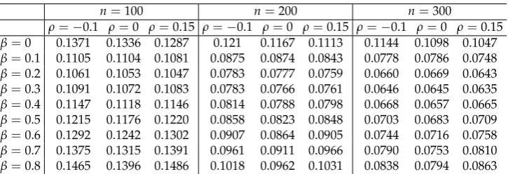
useless. Results are presented in Table1and Table2. Two points deserve our attention. The first one

245

is that, as expected, RMSEs for contaminated data are always greater than RMSEs for pure data and

246

that the RMSEs decrease when the sample sizen increases. The second is that, while in pure data

247

RMSEs are greater for big values of β, when working with contaminated data the CMDPDE with

248

medium-low values ofβ(β∈ {0.1, 0.2, 0.3}) present the best behavior in terms of efficiency.

249

For a nominal sizeα=0.05, with the model under the null hypothesis given in (28), the estimated

250

significance levels for different Wald-type test statistics are given by

b

α(nβ)(ρ0) =Prb(W β

n >χ2_1,0.05|H0) = R

∑

i=1

I(W_nβ_,i)>χ2_1,0.05|ρ0)

R ,

withI(S)being the indicator function (with value 1 ifSis true and 0 otherwise). Empirical levels with

252

the same previous parameter values are presented in Table3(pure data) and Table4(5% of outliers).

253

While medium-high values ofβare not recommended at all, CMLE is the best when working with

254

pure data. However the lack of robustness of CMLE test is impressive, as it can be seen in Table4. The

255

effect of contamination in medium-low values ofβis much lighter, while for medium-high values of

256

βit can return deceptively beneficial.

257

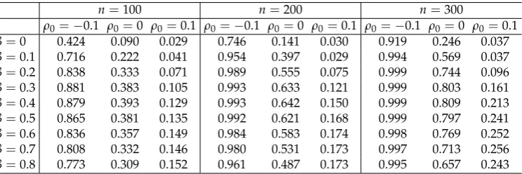
For finite sample sizes and nominal sizeα=0.05, the simulated powers are obtained underH1 258

in (28), whenρ∗ ∈ {−0.1, 0, 0.1}, ˜ρ =0.2 andρ0=0.15 (Table5and Table6). The (simulated) power 259

for different composite Wald-type test statistics is obtained by

260

β(nβ)(ρ0,ρ∗) =Pr(Wnβ >χ2_1,0.05|H1) and βb

(λ)

n (ρ0,ρ∗) =

R

∑

i=1

I(W_nβ_,i>χ2_1,0.05|ρ0,ρ∗)

R .

As expected, when we get closer to the null hypothesis and when decreasing the sample sizes, the

261

power decreases. With pure data the best behavior is obtained withβ = 0 and with contaminated

262

data the best results are obtained for medium values ofβ.

263

Table 1.RMSEs for pure data

n=100 n=200 n=300

ρ=−0.1 ρ=0 ρ=0.15 ρ=−0.1 ρ=0 ρ=0.15 ρ=−0.1 ρ=0 ρ=0.15 β=0 0.0958 0.0950 0.0948 0.0683 0.0668 0.0666 0.0553 0.0552 0.0551 β=0.1 0.0972 0.0961 0.0966 0.0693 0.0676 0.0677 0.0560 0.0559 0.0561 β=0.2 0.1009 0.0991 0.1007 0.0718 0.0697 0.0704 0.0581 0.0575 0.0585 β=0.3 0.1061 0.1034 0.1062 0.0754 0.0727 0.0742 0.0612 0.0599 0.0619 β=0.4 0.1123 0.1087 0.1127 0.0797 0.0762 0.0787 0.0649 0.0628 0.0659 β=0.5 0.1195 0.1147 0.1200 0.0845 0.0803 0.0837 0.0691 0.0661 0.0702 β=0.6 0.1274 0.1215 0.1280 0.0898 0.0848 0.0892 0.0737 0.0697 0.0748 β=0.7 0.1361 0.1291 0.1369 0.0955 0.0897 0.0952 0.0786 0.0736 0.0797 β=0.8 0.1456 0.1374 0.1467 0.1015 0.0905 0.1016 0.0839 0.0778 0.0849

Table 2.RMSEs for contaminated data

n=100 n=200 n=300

ρ=−0.1 ρ=0 ρ=0.15 ρ=−0.1 ρ=0 ρ=0.15 ρ=−0.1 ρ=0 ρ=0.15 β=0 0.1371 0.1336 0.1287 0.121 0.1167 0.1113 0.1144 0.1098 0.1047 β=0.1 0.1105 0.1104 0.1081 0.0875 0.0874 0.0843 0.0778 0.0786 0.0748 β=0.2 0.1061 0.1053 0.1047 0.0783 0.0777 0.0759 0.0660 0.0669 0.0643 β=0.3 0.1091 0.1072 0.1083 0.0783 0.0766 0.0761 0.0646 0.0645 0.0635 β=0.4 0.1147 0.1118 0.1146 0.0814 0.0788 0.0798 0.0668 0.0657 0.0665 β=0.5 0.1215 0.1176 0.1220 0.0858 0.0823 0.0848 0.0703 0.0683 0.0709 β=0.6 0.1292 0.1242 0.1302 0.0907 0.0864 0.0905 0.0744 0.0716 0.0758 β=0.7 0.1375 0.1315 0.1391 0.0961 0.0911 0.0966 0.0790 0.0753 0.0810 β=0.8 0.1465 0.1396 0.1486 0.1018 0.0962 0.1031 0.0838 0.0794 0.0863

4. Conclusions 264

The likelihood function is the basis of the maximum likelihood method in estimation theory and

265

it also plays a key role in the development of log-likelihood ratio tests. However, it is not so tractable

266

in many cases, in practice. Maximum likelihood estimators are based on the likelihood function

267

and they can be easily obtained, however, there are cases where they do not exist or they cannot

Table 3.Levels for pure data

n=100 n=200 n=300

ρ0=−0.1 ρ0=0 ρ0=0.15 ρ0=−0.1 ρ0=0 ρ0=0.15 ρ0=−0.1 ρ0=0 ρ0=0.15

β=0 0.067 0.059 0.070 0.068 0.046 0.062 0.072 0.045 0.075

β=0.1 0.067 0.060 0.072 0.062 0.046 0.070 0.085 0.045 0.079

β=0.2 0.072 0.061 0.084 0.069 0.051 0.084 0.097 0.049 0.102

β=0.3 0.081 0.062 0.093 0.084 0.053 0.100 0.112 0.051 0.121

β=0.4 0.094 0.069 0.099 0.103 0.055 0.111 0.127 0.055 0.142

β=0.5 0.105 0.071 0.111 0.118 0.056 0.122 0.149 0.051 0.155

β=0.6 0.122 0.083 0.129 0.131 0.062 0.136 0.167 0.051 0.165

β=0.7 0.135 0.088 0.141 0.139 0.063 0.146 0.181 0.055 0.177

β=0.8 0.153 0.099 0.158 0.151 0.071 0.156 0.198 0.056 0.179

Table 4.Levels for contaminated data

n=100 n=200 n=300

ρ0=−0.1 ρ0=0 ρ0=0.15 ρ0=−0.1 ρ0=0 ρ0=0.15 ρ0=−0.1 ρ0=0 ρ0=0.15

β=0 0.357 0.223 0.081 0.638 0.429 0.155 0.788 0.623 0.24 0

β=0.1 0.121 0.113 0.056 0.207 0.191 0.077 0.287 0.284 0.100

β=0.2 0.065 0.074 0.048 0.066 0.099 0.049 0.086 0.129 0.059

β=0.3 0.057 0.067 0.071 0.057 0.066 0.059 0.065 0.077 0.073

β=0.4 0.075 0.066 0.087 0.067 0.058 0.081 0.079 0.060 0.095

β=0.5 0.090 0.062 0.107 0.080 0.061 0.110 0.105 0.051 0.128

β=0.6 0.096 0.063 0.126 0.095 0.063 0.131 0.117 0.049 0.151

β=0.7 0.109 0.073 0.137 0.101 0.061 0.141 0.127 0.047 0.159

β=0.8 0.125 0.083 0.147 0.109 0.061 0.149 0.141 0.049 0.171

Table 5.Powers for pure data,ρ∗=0.15

n=100 n=200 n=300

ρ0=−0.1 ρ0=0 ρ0=0.1 ρ0=−0.1 ρ0=0 ρ0=0.1 ρ0=−0.1 ρ0=0 ρ0=0.1

β=0 0.945 0.603 0.141 1 0.871 0.180 1 0.962 0.265

β=0.1 0.954 0.588 0.157 1 0.863 0.207 1 0.96 0.299

β=0.2 0.952 0.557 0.158 1 0.825 0.213 1 0.944 0.315

β=0.3 0.941 0.510 0.153 0.999 0.783 0.213 1 0.913 0.313

β=0.4 0.925 0.465 0.154 0.999 0.734 0.210 1 0.885 0.301

β=0.5 0.904 0.424 0.159 0.996 0.677 0.202 1 0.845 0.289

β=0.6 0.873 0.395 0.153 0.990 0.618 0.197 0.999 0.789 0.277

β=0.7 0.830 0.361 0.153 0.985 0.555 0.183 0.999 0.733 0.261

β=0.8 0.789 0.322 0.161 0.974 0.499 0.179 0.997 0.678 0.246

Table 6.Powers for contaminated data,ρ∗=0.15

n=100 n=200 n=300

ρ0=−0.1 ρ0=0 ρ0=0.1 ρ0=−0.1 ρ0=0 ρ0=0.1 ρ0=−0.1 ρ0=0 ρ0=0.1

β=0 0.424 0.090 0.029 0.746 0.141 0.030 0.919 0.246 0.037

β=0.1 0.716 0.222 0.041 0.954 0.397 0.029 0.994 0.569 0.037

β=0.2 0.838 0.333 0.071 0.989 0.555 0.075 0.999 0.744 0.096

β=0.3 0.881 0.383 0.105 0.993 0.633 0.121 0.999 0.803 0.161

β=0.4 0.879 0.393 0.129 0.993 0.642 0.150 0.999 0.809 0.213

β=0.5 0.865 0.381 0.135 0.992 0.621 0.168 0.999 0.797 0.241

β=0.6 0.836 0.357 0.149 0.984 0.583 0.174 0.998 0.769 0.252

β=0.7 0.808 0.332 0.146 0.980 0.531 0.173 0.997 0.713 0.256

be obtained. In such a case, composite likelihood methods constitute an appealing methodology in

269

the area of estimation and testing of hypotheses. On the other hand, distance or divergence based

270

on methods of estimation and testing have increasingly become fundamental tools in the field of

271

mathematical statistics. The work in [15] is the first, to the best of our knowledge, which links the

272

notion of composite likelihood with divergence based on methods for testing statistical hypotheses.

273

In this paper, MDPDE are introduced and they are exploited to develop Wald type test statistics

274

for testing simple or composite null hypotheses, in a composite likelihood framework. The validity

275

of the proposed procedures is investigated by means of simulations. The simulation results point

276

out the robustness of the proposed information theoretic procedures in estimation and testing, in the

277

composite likelihood context. There are several areas where the notions of divergence and composite

278

likelihood are crucial, including spatial statistics and time series analysis. These are areas of interest

279

and they will be maybe explored elsewhere.

280

Acknowledgments: This research is supported by Grant MTM2015-67057-P, from Ministerio de Economia y 281

Competitividad (Spain). 282

Conflicts of Interest:The authors declare no conflict of interest. 283

Abbreviations 284

The following abbreviations are used in this manuscript: 285

MLE Maximum likelihood estimator

CMLE Composite maximum likelihood estimator DPD Density power divergence

MDPDE Minimum density power divergence estimator

CMDPDE Composite minimum density power divergence estimator 286

Appendix Proof of Results 287

Appendix A.1 Proof of Theorem2 288

The result follows in a straightforward manner because of the asymptotic normality ofbθ β c, 289

√

n(bθ β c−θ0)

L

−→

n→∞N

0,H−_β1(θ0)Jβ(θ0)H

−1 β (θ0)

.

Appendix A.2 Proof of Theorem3 290

A first order Taylor expansion ofl(θ)atbθ β

c aroundθ∗gives 291

lbθ β c

−l(θ∗) =

∂l(θ)

∂θ

θ=θ∗

b θ_cβ−θ∗

+op bθ

β c−θ∗

.

Now the result follows because the asymptotic distribution oflbθ β c

−l(θ∗)

coincides with the

292

asymptotic distribution of√n∂l(θ)

∂θ

θ=θ∗

b θcβ−θ∗

.

293

Appendix A.3 Proof of Theorem5 294

We have

295

g(bθ β

c) = g(θ0) +G(θ0)T

b θβ_c−θ0

+op bθ

β c−θ0

= GT(θ0)

b θβc −θ0

+op bθ

β c−θ0

,

becauseg(θ0)=0r . 296

Therefore

√

ngbθ β c

_L

−→

n−→∞N(0,Gβ(θ0) T_H−1

β (θ0)Jβ(θ0)H

−1

β (θ0)Gβ(θ0))

because

298

√

nbθ β c −θ0

_L

−→

n−→∞N(0,H

−1

β (θ0)Jβ(θ0)H

−1 β (θ0)).

Now

299

Wn,β=ng

b θβ

Th

GT(θ0)H−_β1(θ0)Jβ(θ0)H

−1

β (θ0)G(θ0) i−1

gbθ_β

_L

−→

n−→∞χ 2 r.

Appendix A.4 Computation of Sensitivity and Variability Matrices in the Numerical Example 300

We want to compute

301

H_β(θ) = Z

Rm

CL(θ,y)β+1u(θ,y)Tu(θ,y)dy J_β(θ) =

Z

Rm

CL(θ,y)2β+1u(θ,y)Tu(θ,y)dy

−

Z

Rm

CL(θ,y)β+1u(θ,y)dy Z

Rm

(u(θ,y))TCL(θ,y)β+1dy.

First of all, we can see that

302

CL(θ,y)β+1= fA₁(θ,y)fA2(θ,y) β+1

= 1

2πp1−ρ2

expn−₂₍₁₋1

ρ2)Q(y1,y2)

o

· 1

2πp1−ρ2

expn−₂₍₁₋1

ρ2)Q(y3,y4)

o !β+1

=

₁

(2π)2(1−ρ2)

β+1

expn− β+1

2(1−ρ2)[Q(y1,y2) +Q(y3,y4)]

o

= 1

(β+1)2

1

(2π)2(1−ρ2)

β ₍

β+1)2

(2π)2(1−ρ2)exp

n − β+1

2(1−ρ2)[Q(y1,y2) +Q(y3,y4)] o

=Cβ· CL

∗

β,

whereCβ= 1

(β+1)2

1

(2π)2(1−ρ2) β

andCL∗_β =CL_β(θ,y)∗∼ N(µ,Σ∗), withΣ∗= _β+1₁Σ. 303

304

Whileu(θ,y)= ∂logCL(θ,y)

∂θ we will denote asu(θ,y)

∗

tou(θ,y)∗=

∂logCL∗_β

∂θ . Then

305

u(θ,y)= ∂logCL(θ,y)

∂θ =

1

β+1

∂logCL(θ,y)β+1

∂θ =

1

β+1

∂log(C_β· CL∗_β) ∂θ

= 1

β+1

∂logC_β

∂θ +

∂logCL∗_β

∂θ !

= 1

β+1

_∂logC β

∂θ +u(θ,y)

∗

. (29)

Further,

Z

Rm

CL(θ,y)β+1u(θ,y)dy= Z

Rm

CL(θ,y)β+1∂logCL(θ,y)

∂θ dy=

Z

Rm

CL(θ,y)β∂CL(θ,y)

∂θ dy

= Z

Rm

1

β+1

∂CL(θ,y)β+1

∂θ dy=

1

β+1 ∂

∂θ Z

Rm

CL(θ,y)β+1dy

= 1

β+1 ∂C_β

∂θ = (0, 0, 0, 0,

2ρβC_β

(β+1)(1−ρ2))

T ₌

ξ_β(θ). (30)

Now

307

Z

R4

CLβ+1_u(

θ,y)Tu(θ,y)dy (31) =

Z

R4

(C_β· CL∗_β) 1 (β+1)2

∂logC_β

∂θ +u(θ,y)

∗T∂logCβ

∂θ +u(θ,y)

∗

dy

= Cβ (β+1)2

Z

R4 "

∂logCβ

∂θ

T

∂logCβ

∂θ

CL∗_β

+CL∗_β u(θ,y)∗T

∂logCβ

∂θ +CL

∗

β

∂logCβ

∂θ T

u(θ,y)∗+CL∗_β(u(θ,y)∗)Tu(θ,y)∗ #

dy

= Cβ (β+1)2

"

∂logCβ

∂θ

T

∂logCβ

∂θ Z

R4

CL∗_βdy+ Z

R4

CL∗_βu(θ,y)∗dy T

∂logCβ

∂θ

+

∂logCβ

∂θ TZ

R4

CL∗_βu(θ,y)∗dy+ Z

R4

CL∗_β(u(θ,y)∗)Tu(θ,y)∗dy #

= Cβ (β+1)2

" KTK+

Z

R4

CL∗_βu(θ,y)∗dy T

K+KT Z

R4

CL∗_βu(θ,y)∗dy+ Z

R4

CL∗_β(u(θ,y)∗)Tu(θ,y)∗dy #

,

whereK= ∂logCβ

∂θ = (0, 0, 0, 0, 2ρ·β 1−ρ2). But 308

Z

R4

CL∗_βu(θ,y)∗dy= Z

R4

1

Cβ

CL(θ,y)β+1 !

(β+1)u(θ,y)−

∂logC_β ∂θ

dy

= β+1 Cβ

Z

R4

CL(θ,y)β+1u(θ,y)dy

− K

Cβ Z

R4

CL(θ,y)β+1dy

= 1 Cβ

∂C_β

∂θ −K=K−K=0,

and thus (31) can be expressed as

309

Z

R4

CL(θ,y)β+1u(θ,y)Tu(θ,y)dy= C_β (β+1)2

KTK+

Z

R4

CL∗_β(u(θ,y)∗)Tu(θ,y)∗dy

.

On the other hand, it is not difficult to prove that

310

Z

R4

CL∗_β(u(θ,y)∗)Tu(θ,y)∗dy=C· Z

R4

CL(θ,y)(u(θ,y))Tu(θ,y)dy=C·H0(θ),

whereC=diag(β+1,β+1,β+1,β+1, 1)and ([15])

H0(θ) = 

        

1 1−ρ2

−ρ

1−ρ2 0 0 0

−ρ 1−ρ2

1

1−ρ2 0 0 0

0 0 ₁₋1

ρ2

−ρ 1−ρ2 0

0 0 −ρ

1−ρ2 1

1−ρ2 0

0 0 0 0 2(ρ2+1)

(1−ρ2)2 

        

. (32)

So

312

Hβ(θ) = C_β (β+1)2

h

C·H0(θ) +KTK i

,

this is

313

Hβ(θ) =

Cβ (β+1)(1−ρ2)



      

1 −ρ 0 0 0

−ρ 1 0 0 0

0 0 1 −ρ 0

0 0 −ρ 1 0

0 0 0 0 2(ρ2+1)+2ρ2β2

(1−ρ2)(1+β) 

      

. (33)

Note that, forβ=0, (33) equals to (32).

314

On the other hand, the expression of the variability matrix J_β(θ) can be obtained from 315

expressions (26) and (30) as

316

J_β(θ) =H2β(θ)−ξβ(θ) T

ξ_β(θ). (34)

References 317

1. Basu, A.; Harris, I.R.; Hjort, N.L. and Jones, M.C. Robust and efficient estimation by minimizing a density 318

power divergence.Biometrika,1998,85, 549–559. 319

2. Basu, A.; Mandal, A.; Martín, N. and Pardo, L. Testing statistical hypotheses based on the density power 320

divergence.Ann. Inst. Stat. Math.,2013,65, 319–348 321

3. Basu, A.; Mandal, A.; Martín, N. and Pardo, L. Robust tests for the equality of two normal means based on 322

the density power divergence.Metrika,2015,78, 611–634. 323

4. Basu, A.; Mandal, A.; Martín, N. and Pardo, L. Generalized Wald-type tests based on minimum density 324

power divergence estimators.Statistics,2016,50, 1, 1-26. 325

5. Basu, A.; Ghosh, A. Mandal; Martín, N. and Pardo, L. A Wald-type test statistic for testing linear hypothesis 326

in logistic regression models based on minimum density power divergence estimator.Electon. J. Stat.,2017, 327

11, 2, 2741–2772. 328

6. Ghosh, A.; Mandal, A.; Martín, N. and Pardo, L. Influence analysis of robust Wald-type tests.J. Multivariate 329

Anal.,2016,147, 102–126. 330

7. Varin, C.; Reid, N. and Firth, D. An overview of composite likelihood methods.Stat. Sin.,2011,21, 1, 4-42. 331

8. Xu, X. and Reid, N. On the robustness of maximum composite estimate.J. Stat. Plan. Inference.,2011,141, 332

3047-3054. 333

9. Joe, H., Reid, N.; Somg, P.X.; Firth, D. and Varin, C. Composite likelihood methods.Report on the Workshop 334

on Composite Likelihood.2012Available at http://www.birs.ca/events/2012/5-day-workshops/12w5046. 335

10. Lindsay, G. Composite likelihood methods.Contemp. Math.,1998,80, 221-239. 336

11. Basu, A.; Shioya, H. and Park, C.Statistical inference. The minimum distance approach. Chapman & Hall/CRC. 337

Boca Raton, 2011. 338

12. Maronna, R. A., Martin, R. D. and Yohai, V. J. Time Series, in Robust Statistics: Theory and Methods, John 339

Wiley & Sons, Ltd, Chichester, UK., 2006. 340

13. Pardo, L.Statistical inference based on divergence measures. Chapman & Hall/CRC. Boca Raton, 2006. 341

15. Martín, N.; Pardo, L. and Zografos, K. On divergence tests for composite hypotheses under composite 343