Processing of higher count rates in Troitsk nu-mass experiment
AlexanderNozik1,2,and VaslilyChernov1
1Institute for Nuclear Research RAS, prospekt 60-letiya Oktyabrya 7a, Moscow 117312
2Moscow Institute of Physics and Technology, 9 Institutskiy per., Dolgoprudny, Moscow Region, 141700, Russian Federation
Abstract. In this article we give a short outline of current status of search for sterile neutrinos with masses up to 4 keV in “Troitsk nu-mass experiment”. We also discuss major sources of systematic uncertainties and methods to lower them.
1 Introduction
Neutrino studies are one of the most motivating research areas in modern particle physics. While the particle itself was theoretically proposed in 1930-s, neutrino exact properties are still not known. Due to very small interaction cross-section, neutrino proved to be very hard to study experimentally. For now, one of the most interesting question is the absolute mass scale of neutrinos. The discovery of neutrino oscillations points to the fact that neutrino mass is not zero, but direct measurements still provide only upper limits for its mass of about 2 eV ([1]).
Additional point of interest is the search for so-called sterile neutrinos (special type of neutrino that does not participate in weak interaction). There is a number of indirect indications that such sterile neutrinos could exist ([2]), but there is almost no direct knowledge about specific region of masses or mixing parameters.
2 Troitsk nu-mass experiment
Troitsk nu-mass experiment detailed description as well as sterile neutrino program proposal could be found in [3]. The recent results for sterile neutrino with mass up to 1 keV are published in [4].
The main complication of search for sterile neutrino compared to search for electron neutrino mass performed previously in Troitsk nu-mass experiment ([1][5]) is the broader energy region. It produces two additional problems:
• The uncertainty caused by imprecise knowledge of electronics dead time.
• The uncertainty due to different number of events under the detector threshold for different retarding potentials.
The second problem is caused by back scattering effects discussed in [6] and could be solved only with precise simulations. In this article we will discuss the first problem and ways to solve it.
3 Reducing dead time uncertainty
The current DAQ hardware, used in the Troitsk nu-mass has a dead time of approximately 6.5µs. It
was sufficient for count rates of about 100 Hz used when the spectrum endpoint was investigated in search for electron neutrino mass ([1]). However, at count rates required to get sufficient statistics for sterile neutrino search (20 – 40 kHz) even small deviations of estimated dead time could produce huge differences in count rate (see systematic uncertainties estimation in [7]). Furthermore, since dead time was determined by analog readout system, it could be precisely estimated only experimentally.
3.1 Continuous digitization
One of possible solutions to reduce the impact of dead time uncertainty is to reduce dead time itself. It could be done either by using faster electronics, or by using advanced signal shape analysis to designate pileup events in off-line analysis. The first approach is currently impossible to implement on Troitsk nu-mass because shorter shaping times introduce additional systematic error caused by additional events from detector back scattering (discussed in [6]). Therefore it was decided to switch to continuous digitization without changing shaping time.
There were two candidates for digitization hardware: CAEN DT-5270 and Rudnev-Shilaev Lan10-12PCI. DT-5270 allowed for much faster sampling rate (31.25 MHz and higher), but it proved to be unsuitable for continuous digitization due to limitations of computer interface (USB channel band-width limit of 30 mb/s). Lan10-12PCI, on the other hand, provides much lower sampling rate and have direct PCI-express interface with the computer bus. It was discovered that optimal Lan10-12PCI performance could be obtained with sampling rate of 3.125 MHz. In that case live time losses due to data download to computer amounts only to about 13%.
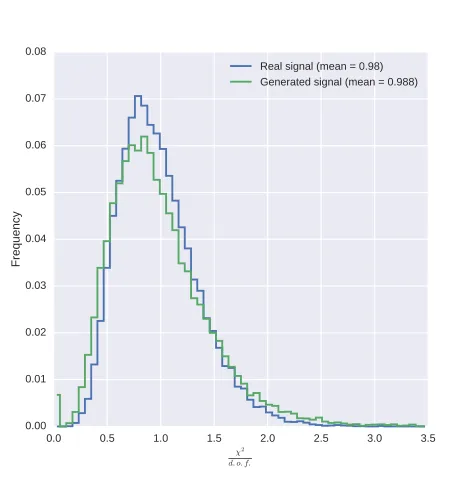
Additional benefit of continuous digitization is the ability to simulate exact pile up effect using known signal shape. In order to do so one need to introduce an artificial signal and background noise distribution indistinguishable from real experimental data. In order to check the quality of analytic signal shape as well as background distribution, we plotted the distribution ofχ2 over degree of
freedom for experimental and simulated data versus analytic signal shape in Fig. 1.
It could be clearly seen, that both shapes are very similar and produce very good average quality of fit.
Three different algorithms were considered for off-line analysis of the signal shape:
1. Direct search for local peaks. This is the simplest and fastest method. However, it has rather high miss rate for close events because one needs a clear local minimum between events to separate them.
2. Search for local peaks with compensation. This method is a modification of the first one. In this case when the peak is found, it is reconstructed using analytic signal shape and subtracted from the initial signal to reduce influence on subsequent peaks.
3. Signal front fit. In this case reconstruction of signal performed not by finding its peak, but by fitting its front with analytical shape.
3 Reducing dead time uncertainty
The current DAQ hardware, used in the Troitsk nu-mass has a dead time of approximately 6.5µs. It
was sufficient for count rates of about 100 Hz used when the spectrum endpoint was investigated in search for electron neutrino mass ([1]). However, at count rates required to get sufficient statistics for sterile neutrino search (20 – 40 kHz) even small deviations of estimated dead time could produce huge differences in count rate (see systematic uncertainties estimation in [7]). Furthermore, since dead time was determined by analog readout system, it could be precisely estimated only experimentally.
3.1 Continuous digitization
One of possible solutions to reduce the impact of dead time uncertainty is to reduce dead time itself. It could be done either by using faster electronics, or by using advanced signal shape analysis to designate pileup events in off-line analysis. The first approach is currently impossible to implement on Troitsk nu-mass because shorter shaping times introduce additional systematic error caused by additional events from detector back scattering (discussed in [6]). Therefore it was decided to switch to continuous digitization without changing shaping time.
There were two candidates for digitization hardware: CAEN DT-5270 and Rudnev-Shilaev Lan10-12PCI. DT-5270 allowed for much faster sampling rate (31.25 MHz and higher), but it proved to be unsuitable for continuous digitization due to limitations of computer interface (USB channel band-width limit of 30 mb/s). Lan10-12PCI, on the other hand, provides much lower sampling rate and have direct PCI-express interface with the computer bus. It was discovered that optimal Lan10-12PCI performance could be obtained with sampling rate of 3.125 MHz. In that case live time losses due to data download to computer amounts only to about 13%.
Additional benefit of continuous digitization is the ability to simulate exact pile up effect using known signal shape. In order to do so one need to introduce an artificial signal and background noise distribution indistinguishable from real experimental data. In order to check the quality of analytic signal shape as well as background distribution, we plotted the distribution ofχ2 over degree of
freedom for experimental and simulated data versus analytic signal shape in Fig. 1.
It could be clearly seen, that both shapes are very similar and produce very good average quality of fit.
Three different algorithms were considered for off-line analysis of the signal shape:
1. Direct search for local peaks. This is the simplest and fastest method. However, it has rather high miss rate for close events because one needs a clear local minimum between events to separate them.
2. Search for local peaks with compensation. This method is a modification of the first one. In this case when the peak is found, it is reconstructed using analytic signal shape and subtracted from the initial signal to reduce influence on subsequent peaks.
3. Signal front fit. In this case reconstruction of signal performed not by finding its peak, but by fitting its front with analytical shape.
The results of simulations of different methods effectiveness for count rate about 40 kHz are shown in table 1. Front fit method, as expected, gives better results for pileup recognition, but it produces a lot of false positive signals. Also it gives much worse performance then other two. Both methods 1 and 2 give similar effectiveness and performance. Further tests showed that using either of these methods produce an effective dead time caused by indistinguishable pile-up events of about 2.1µs
Figure 1: Distributions ofχ2 over degree of freedom for simulated and experimental events versus analytic signal shape.
Direct Direct with correction Front fit Computation time, s 1.222999 3.176033 195.431107
Total events 80526 80526 80526
Recognized events 72174 72244 79067
False negatives 1358 1269 467
False positives 6 4 1767
Pileup 6467 6470 2607
Table 1: Comparison of different peak recognition methods
which is almost 3 times better than the dead time of analog system. Furthermore, computation time of 1-3 s for 2 s measurement after optimization will allow to use these algorithms on-line to reduce stored data size.
3.2 Statistical approach
Another approach to dead time problem is to use information on events time distribution. The distri-bution of time delays between signals follows exponential distridistri-bution:
f(t)= 1
τe
−t/τ, (1)
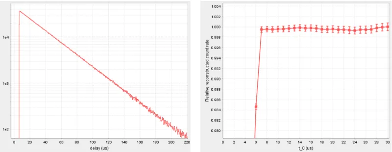
(a) Histogram of delays between events for dead time of
6.5µs. (b) Reconstructed count rate with error for di
fferent
cut-offtimest0(inµs.)
Figure 2: Statistical count rate reconstruction of simulated data.
Let us consider that there is sharp dead time margint0that does not allow two events to be closer in time than thist0. In this case the shape of time distribution abovet0wont change, but there will be change in distribution normalization:
f∗(t)=et0/τ τ
e−t/τ t≥t
0
0 t<t0 (2)
In order to avoid uncertainties from electronics dead time, one could select a t0 slightly above the apparatus cutoffand estimate τusing modified distribution f∗(t). Sincet0 is artificial, it could
be selected with any needed precision and does not produce additional systematic error. Of course statistical error will be slightly increased because some events with delay belowt0are excluded from analysis.
To get estimate ofτone can use the maximum likelihood method. The likelihood function for modified distribution could be written in a following way:
L(τ)=
N
i=1 f(ti)=
et0/τ
τ N
exp
−1τ
N
i=1 ti
, (3)
wheretiare experimental times between events greater thent0andN is total number of events with
t>t0. DesignatingiN=1tiasT, the likelihood logarithm could be written in a following way:
lnL(τ)∼ −Nlnτ−1
τ(T−Nt0) (4)
The maximum ofL(τ) corresponds to
τ0= TN −t0. (5)
The difference between regular exponential distribution and modified one is additional shiftt0. The statistical uncertainty forτ0is defined by the same formula as for regular oneστ0=τ0/
√
(a) Histogram of delays between events for dead time of
6.5µs. (b) Reconstructed count rate with error for di
fferent
cut-offtimest0(inµs.)
Figure 2: Statistical count rate reconstruction of simulated data.
Let us consider that there is sharp dead time margint0that does not allow two events to be closer in time than thist0. In this case the shape of time distribution abovet0wont change, but there will be change in distribution normalization:
f∗(t)=et0/τ τ
e−t/τ t≥t
0
0 t<t0 (2)
In order to avoid uncertainties from electronics dead time, one could select a t0 slightly above the apparatus cutoffand estimate τusing modified distribution f∗(t). Sincet0 is artificial, it could
be selected with any needed precision and does not produce additional systematic error. Of course statistical error will be slightly increased because some events with delay belowt0are excluded from analysis.
To get estimate ofτone can use the maximum likelihood method. The likelihood function for modified distribution could be written in a following way:
L(τ)=
N
i=1 f(ti)=
et0/τ
τ N
exp
−1τ
N
i=1 ti
, (3)
wheretiare experimental times between events greater thent0andN is total number of events with
t>t0. DesignatingiN=1tiasT, the likelihood logarithm could be written in a following way:
lnL(τ)∼ −Nlnτ−1
τ(T−Nt0) (4)
The maximum ofL(τ) corresponds to
τ0= TN −t0. (5)
The difference between regular exponential distribution and modified one is additional shift t0. The statistical uncertainty forτ0is defined by the same formula as for regular oneστ0=τ0/
√
N. The
ratio between statistical error for the whole data set and for cut one equals the square root of ratio between total number of events before and after the cut. For count rates up to 30 - 40 kHz andt0about 5-10µsone can completely eradicate systematic error from the dead time, sacrificing only 10-15% of statistic sensitivity.
Fig. 2a shows the histogram of delays between subsequent events for a count rate of 30 kHz with a dead time of 6.5µs. Fig. 2b shows count rate reconstructed via statistical procedure for different
values oft0. It could be clearly seen, that fort0 above real dead time, the value of reconstructed rate suffers only slight fluctuations well within statistical errors and for higher values oft0errors are
actually larger.
4 Conclusion
The combination of continuous digitization and statistical count rate estimation allow to significantly decrease the systematic error from dead time. The second primary source of uncertainty: events under the threshold, requires additional study and simulations. Algorithms used to distinguish pileup events could be optimized to be used on-line, thus allowing to use continuous digitization not only for one-pixel detector, but also for detectors with a lot of pixels without developing complicated storage system.
The work was supported by RFBR grant 17-02-00361 A. Authors would like to thank the whole Troitsk nu-mass group and particularly its leader Vladislav Pantuev.
References
[1] V.N. Aseev et al. (Troitsk), Phys. Rev.D84, 112003 (2011),1108.5034
[2] R. Adhikari et al., Submitted to: White paper (2016),1602.04816
[3] D. Abdurashitov, A. Belesev, A. Berlev, V. Chernov, E. Geraskin, A. Golubev, G. Koroteev, N. Likhovid, A. Lokhov, A. Markin et al., arXiv preprint arXiv:1504.00544 (2015)
[4] J.N. Abdurashitov et al., JETP Lett.105, 753 (2017),1703.10779
[5] A.I. Belesev, A.I. Berlev, E.V. Geraskin, A.A. Golubev, N.A. Likhovid, A.A. Nozik, V.S. Pantuev, V.I. Parfenov, A.K. Skasyrskaya, J. Phys.G41, 015001 (2014),1307.5687
[6] P.V. Grigorieva, A.A. Nozik, V.S. Pantuev, A.K. Skasyrskaya (2015),1511.06129