How to Certify the Leakage of a Chip?
Fran¸cois Durvaux, Fran¸cois-Xavier Standaert, Nicolas Veyrat-Charvillon UCL Crypto Group, Universit´e catholique de Louvain.
Place du Levant 3, B-1348, Louvain-la-Neuve, Belgium.
Abstract. Evaluating side-channel attacks and countermeasures requires determining the amount of information leaked by a target device. For this purpose, information extraction procedures published so far essentially combine a “leakage model” with a “distinguisher”. Fair evaluations ide-ally require exploiting a perfect leakage model (i.e. exactly corresponding to the true leakage distribution) with a Bayesian distinguisher. But since such perfect models are generally unknown, density estimation tech-niques have to be used to approximate the leakage distribution. This raises the fundamental problem that all security evaluations are poten-tially biased by both estimation and assumption errors. Hence, the best that we can hope is to be aware of these errors. In this paper, we provide and implement methodological tools to solve this issue. Namely, we show how sound statistical techniques allow both quantifying the leakage of a chip, and certifying that the amount of information extracted is close to the maximum value that would be obtained with a perfect model.
1
Introduction
Side-channel attacks aim to extract secret information from cryptographic im-plementations. For this purpose, they essentially compare key-dependent leakage models with actual measurements. As a result, models that accurately describe the target implementation are beneficial to the attack’s efficiency.
More formally, the relation between accurate leakage models and fair security analyses is also central in evaluation frameworks such as proposed at Eurocrypt 2009 [33]. In particular, this previous work established that the leakage of an implementation (or the quality of a measurement setup) can be quantified by measuring the Mutual Information (MI) between the secret cryptographic keys manipulated by a device and the actual leakage produced by this device. Un-fortunately, the design of unbiased and non-parametric estimators for the MI is a notoriously hard problem. Yet, since the goal of side-channel attacks is to use the “best available” models in order to recover information, a solution is to estimate the MI based on these models. This idea has been precised by Renauld et al. with the notion of Perceived Information (PI) - that is nothing else than an estimation of the MI biased by the side-channel adversary’s model [27]. Intu-itively, the MI captures the worst-case security level of an implementation, as it corresponds to an (hypothetical) adversary who can perfectly profile the leakage Probability Density Function (PDF). By contrast, the PI captures its practical counterpart, where actual estimation procedures are used to profile the PDF. Our contribution. The previous formal tools provide a sound basis for dis-cussing the evaluation question “how good is my leakage model?”. The answer to this question actually corresponds to the difference between the MI and the PI. Nevertheless, we remain with the problem that the MI is generally unknown (just as the actual leakage PDF), which makes it impossible to compute this dif-ference directly. Interestingly, we show in this paper that it is possible to perform sound(er) security analyses, where the approximations used by the side-channel evaluators are quantified, and their impact on security is kept under control.
In this context, we start with the preliminary observation that understanding these fair evaluation issues requires to clearly distinguish between estimation er-rors and assumption erer-rors, leading to three main contributions. First, we show how cross–validation can be used in order to precisely gauge the convergence of an estimated model. Doing so, we put forward that certain evaluation metrics (e.g. Pearson’s correlation or PI) are better suited for this purpose. Second, we propose a method for measuring assumption errors in side-channel attacks, tak-ing advantage of the distance sampltak-ing technique introduced in [39]. We argue that it allows detecting imperfect hypotheses without any knowledge of the true leakage distribution1! Third, we combine these tools in order to determine the probability that a model error is due to estimation or assumption issues. We then discuss the (im)possibility to precisely (and generally) bound the result-ing information loss. We also provide pragmatic guidelines for physical security evaluators. For illustration, we apply these contributions to actual measurements obtained from an AES implementation in an embedded microcontroller. As a re-sult and for the first time, we are able to certify that the leakage of a chip (i.e. its worst-case security level) is close to the one we are able to extract.
1 By contrast, the direct solution for quantifying the PI/MI distance would be to
These results have implications for the certification of any cryptographic product against side-channel attacks - as they provide solutions to guarantee that the evaluation made by laboratories is based in sound assumptions. They could also be used to improve the comparison of measurement setups such as envisioned by the DPA contest v3 [8]. Namely, this contest suggests comparing the quality of side-channel measurements with a CPA based on an a-priori leakage model. But this implies that the best traces are those that best comply with this a-priori, independent of their true informativeness. Using the PI to compare the setups would already allow each participant to choose his leakage assumptions. And using the cross–validation and distance sampling techniques described in this work would allow determining how relevant these assumptions are.
Notations. We use capital letters for random variables, small caps for their realizations, sans serif fonts for functions and calligraphic letters for sets.
2
Background
2.1 Measurement setups
Our experiments are based on measurements of an AES Furious implementation2 run by an 8-bit Atmel AVR (AtMega 644p) microcontroller at a 20 MHz clock frequency. Since the goal of this paper is to analyze leakage informativeness and model imperfections, we compared traces from three different setups. First, we considered two types of “power-like” measurements. For this purpose, we moni-tored the voltage variations across both a 22Ω resistor and a 2µH inductance introduced in the supply circuit of our target chip. Second, we captured the elec-tromagnetic radiation of our target implementation, using a Rohde & Schwarz (RS H 400-1) probe - with up to 3 GHz bandwidth - and a 20 dB low-noise am-plifier. Measurements were taken without depackaging the chip, hence providing no localization capabilities. Acquisitions were performed using a Tektronix TDS 7104 oscilloscope running at 625 MHz and providing 8-bit samples. In practice, our evaluations focused on the leakage of the first AES master key byte (but would apply identically to any other enumerable target). Leakage traces were produced according to the following procedure. Letxandsbe our target input plaintext byte and subkey, and y =x⊕s. For each of the 256 values of y, we generated 1000 encryption traces, where the rest of the plaintext and key was random (i.e. we generated 256 000 traces in total, with plaintexts of the shape p=x||r1||. . .||r15, keys of the shapek=s||r16||. . .||r30, and theri’s denoting uniformly random bytes). In order to reduce the memory cost of our evalua-tions, we only stored the leakage corresponding to the 2 first AES rounds (as the dependencies in our target byte y = x⊕s typically vanish after the first round, because of the strong diffusion properties of the AES). In the following, we will denote the 1000 encryption traces obtained from a plaintextpincluding the target bytexunder a keykincluding the subkeysas:AESks(px) l
i y (with
2
i∈[1; 1000]). Furthermore, we will refer to the traces produced with the resistor, inductance and EM probe as lr,i
y , lly,i and lemy,i. Eventually, whenever accessing the points of these traces, we will use the notation li
y(j) (with j ∈ [1; 10 000], typically). These subscripts and superscripts will omitted when not necessary.
2.2 Evaluation metrics
In this subsection, we recall a few evaluation metrics that have been introduced in previous works on side-channel attacks and countermeasures.
Correlation coefficient (non-profiled).In view of the popularity of the CPA distinguisher in the literature, a natural candidate evaluation metric is Pear-son’s correlation coefficient. In a non-profiled setting, an a-priori (e.g. Hamming weight) model is used for computing the metric. The evaluator then estimates the correlation between his measured leakages and the modeled leakages of a target intermediate value. In our AES example and targeting an S-box output, it would lead to ˆρ(LY,model(Sbox(Y))), where the “hat” notation is used to denote the estimation of a statistic. In practice, this estimation is performed by sampling (i.e. measuring)Nt“test” traces from the leakage distributionLY. In the following, we will denote the set of theseNttest traces asLtY.
Correlation coefficient (profiled).In order to avoid possible biases due to an incorrect a-priori choice of leakage model, a natural solution is to extend the pre-vious proposal to a profiled setting. In this case, the evaluator will start by build-ing a model from Np “profiling” traces. We denoted this step as modelˆ ρ← LpY (withLpY ⊥⊥ Lt
Y). In practice, it is easily obtained by computing the sample mean values of the leakage points corresponding to the target intermediate values. Signal-to-Noise Ratio (SNR).Yet another solution put forward by Mangard is to compute the SNR of the measurements [20], defined as:
ˆ
SNR=varˆ y(ˆEi(L i y)) ˆ
Ey( ˆvari(Liy)) ,
where ˆEand ˆvar denote the sample mean and variance of the leakage variable, that are estimated from theNttraces inLtY (like the correlation coefficient). Perceived information.Eventually, as mentioned in introduction the PI can be used for evaluating the leakage of a cryptographic implementation. Its sample definition (that is most useful in evaluations of actual devices) is given by:
ˆ
PI(S;X, L) = H[S]−X
s∈S
Pr[s]X x∈X
Pr[x] X li
y∈LtY
Prchip[liy|s, x].log2Prˆmodel[s|x, liy],
where ˆPrmodel ← L
p
Under the assumption that the model is properly estimated, it is shown in [19] that the three latter metrics are essentially equivalent in the context of standard univariate side-channel attacks (i.e. exploiting a single leakage point li
y(j) at a time). By contrast, only the PI naturally extends to multivariate attacks [36]. It can be interpreted as the amount of information leakage that will be exploited by an adversary using an estimated model. So just as the MI is a good predictor for the success rate of an ideal TA exploiting the perfect model Prchip, the PI
is a good predictor for the success rate of an actual TA exploiting the “best available” model ˆPrmodel obtained through the profiling of a target device.
2.3 PDF estimation methods
Computing metrics such as the PI defined in the previous section requires one to build a probabilistic leakage model ˆPrmodel for the leakage behavior of the device. We now describe a few techniques that can be applied for this purpose. Gaussian templates.The seminal TA in [7] relies on an approximation of the leakages using a set of normal distributions. That is, it assumes that each inter-mediate computation generates samples according to a Gaussian distribution. In our typical scenario where the targets follow a key addition, we consequently use:
ˆ
Prmodel[ly|s, x] ≈ Prˆmodel[ly|s⊕x] ∼ N(µy, σy2). This approach simply requires estimating the sample means and variances for each value of y = x⊕s (and mean vectors / covariance matrices in case of multivariate attacks).
Regression-based models.To reduce the data complexity of the profiling, an alternative approach proposed by Schindler et al. is to exploit Linear Regres-sion (LR) [29]. In this case, a stochastic model ˆθ(y) is used to approximate the leakage function and built from a linear basis g(y) = {g0(y), ...,gB−1(y)} cho-sen by the adversary/evaluator (usually gi(y) are monomials in the bits of y). Evaluating θ(ˆy) boils down to estimating the coefficients αi such that the vec-tor ˆθ(y) =P
jαjgj(y) is a least-square approximation of the measured leakages Ly. In general, an interesting feature of such models is that they allow trading profiling efforts for online attack complexity, by adapting the basis g(y). That is, a simpler model with fewer parameters will converge for smaller values ofNp, but a more complex model can potentially approximate the real leakage func-tion more accurately. Compared to Gaussian templates, another feature of this approach is that only a single variance (or covariance matrix) is estimated for capturing the noise (i.e. it relies on an assumption of homoscedastic errors). Histograms and Kernels. See appendix A.
3
Estimation errors and cross–validation
Estimating the PI from a leaking implementation essentially holds in two steps. First, a model has to be estimated from a set of profiling traces LpY: ˆPrmodel←
LpY. Second, a set of test tracesLt
true distribution Prchip[li
y|s, x]). As a result, two main model errors can arise. First, the number of traces in the profiling set may be too low to estimate the model properly. This corresponds to the estimation errors that we analyze in this section. Second, the model ˆPrmodel may not be able to predict the distribution
of samples in the test set, even after intensive profiling. This corresponds to the assumption errors that will be analyzed in the next section. In both cases, such model errors will be reflected by a divergence between the PI and MI.
In order to verify that estimations in a security evaluation are sufficiently accurate, the standard solution is to exploit cross–validation. In general, this technique allows gauging how well a predictive (here leakage) model performs in practice [13]. In the rest of the paper, we use 10-fold cross–validations for illus-tration (which is commonly used in the literature [11]). What this means is that the set of acquired tracesLY is first split into ten (non overlapping) setsL
(i) Y of approximately the same size. Let us define the profiling setsLp,(j)Y =S
i6=jL (i) Y and the test sets Lt,(j)Y =LY \ L
p,(j)
Y . The sample PI is then repeatedly com-puted ten times for 1≤j ≤10 as follows. First, we build a model from a profiling set: ˆPr(j)model ← Lp,(j)Y . Then we estimate ˆPI(j)(S;X, L) with the associated test set Lt,(j)Y . Cross–validation protects us from obtaining too large PI values due to over-fitting, since the test computations are always performed with an inde-pendent data set. Finally, the 10 outputs can be averaged to get an unbiased estimate, and their spread characterizes the accuracy of the result3.
3.1 Experimental results
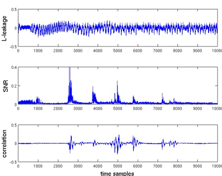
As a starting point, we represented illustrative traces corresponding to our three measurement setups in Appendix B, Figure 10, 11, 12. The figures further contain the SNRs and correlation coefficients of a CPA using Hamming weight leakage model and targeting the S-box output. While insufficient for fair security evalua-tions as stated below, these metrics are interesting preliminary steps, since they indicate the parts of the traces where useful information lies. In the following, we extract a number of illustrative figures from meaningful samples.
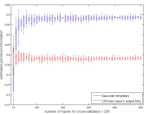
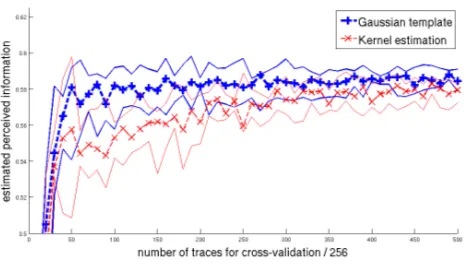
From a methodological point of view, the impact of cross–validation is best represented with the box plot of Figure 1: it contains the PI of point 2605 in the resistor-based traces, estimated with Gaussian templates and a stochastic model using a 17-element linear basis for the bits of the S-box input and output. This point is the most informative one in our experiments (across all measure-ments and estimation procedures we tried). Results show that the PI estimated with Gaussian templates is higher - hence suggesting that the basis used in our regression-based profiling was not fully reflective of the chip activity for this
3 Cross–validation can also apply to profiled CPA, by building modelsmodelˆ
ρ← Lp,Y(j),
Fig. 1.Perceived information estimated from Gaussian templates and LR-based mod-els, with cross–validation (target point 2605 from the resistor-based measurements).
sample. More importantly, we observe that the estimation converges quickly (as the spread of our 10 PI estimates decreases quickly with the number of traces). As expected, this convergence is faster for regression-based profiling, reflecting the smaller number of parameters to estimate in this case. Note that we also per-formed this cross–validation for the Kernel-based PDF estimation described in Appendix A (see Appendix B, Figure 13 for the results). Both the expected value of the PI and its spread suggest that these two density estimation techniques provide equally satisfying results in our implementation context.
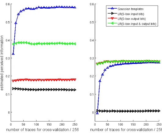
mea-Fig. 2. PI for different PDF estimation techniques and two leakage (resistor-based) points. Left: most informative one (2605), right: other point of interest (4978).
sured with two different (yet similar) measurement setups. Many variations of such evaluations are possible (for more samples, estimation procedures, . . . ). For simplicity, we will limit our discussion to the previous examples, and use them to further discuss the critical question of assumption errors in the next section.
4
Assumption errors and distance sampling
Looking at Figures 1 and 2, we can conclude that our estimation of the PI is reasonably accurate and that Gaussian templates are able to extract a given amount of information from the measurements. Nevertheless, such pictures still do not provide any clue about the closeness between our estimated PI and the (true, unknown) MI. As previously mentioned in introduction, evaluating the deviation between the PI and MI is generally hard. In theory, the standard approach for evaluating such a deviation would be to compute a statistical (e.g. Kullback-Leibler) distance ˆDKL( ˆPrmodel,Prchip). But this requires knowing the
(unknown) distribution Prchip, leading to an obvious chicken and egg problem.
Smirnov [6] or Cram´er–von–Mises [1]), much fewer solutions exist that gener-alize to multivariate statistics. Since we additionally need a test that applies to any distribution, possibly dealing with correlated leakage points, a natural proposal is to exploit statistics based on spacings (or interpoint distance) [24]. The basic idea of such a test is to reduce the dimensionality of the problem by comparing the distributions of distances between pairs of points, consequently simplifying it into a one-dimensional goodness-of-fit test again. It exploits the fact that two multidimensional distributionsF andGare equal if and only if the variables X ∼ F and Y ∼ G generate identical distributions for the distances
D(X1,X2),D(Y1,Y2) andD(X3,Y3) [3, 14]. In our evaluation context, we can
simply check if the distance between pairs of simulated samples (generated with a profiled model) and the distance between simulated and actual samples behave differently. If the model estimated during the profiling phase of a side-channel attack is accurate, then the distance distributions should be close. Otherwise, there will be a discrepancy that the test will be able to detect, as we now detail. The first step of our test for the detection of incorrect assumptions is to compute the simulated distance cumulative distribution as follows:
fsim(d, s, x) = PrhL1y−L2y ≤d L
1 y, L
2
y∼Prˆmodel[Ly|s, x] i
.
Since the evaluator has an analytical expression for ˆPrmodel, this cumulative
dis-tribution is easily obtained. Next, we compute the sampled distance cumulative distribution from the test sample setLt
Y as follows: ˆ
gNt(d, s, x) = Pr h
liy−ljy≤d
liy
1≤i≤Nt ∼ ˆ
Prmodel[Ly|s, x],lyj 1≤j≤Nt =L t Y
i .
Eventually, we need to detect how similarfsimandgNt are, which is made easy since these cumulative distributions are now univariate. Hence, we can compute the distance between them by estimating the Cram´er–von–Mises divergence:
ˆ
CvM(fsim,gˆNt) = Z ∞
−∞
[fsim(x)−gˆNt(x)] 2
dx.
As the number of samples in the estimation increases, this divergence should gradually tend towards zero provided the model assumptions are correct.
4.1 Experimental results
As in the previous section, we applied cross–validation in order to compute the Cram´er–von–Mises divergence between the distance distributions. That is, for each of the 256 target intermediate values, we generated 10 different estimates ˆ
gN(j)
t(d, s, x) and computed ˆ
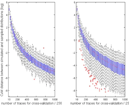
CvM(j)(fsim,ˆgNt) from them. An exemplary evalua-tion is given in Figure 3 for the same leakage point and estimaevalua-tion methods as in Figure 1. For simplicity, we plotted a picture containing the 256 (av-erage) estimates at once4. It shows that Gaussian templates better converge
4
Fig. 3. Cram´er–von–Mises divergence between simulated and sampled distributions, with cross–validation (target point 2605 from the resistor-based measurements). Left: Gaussian templates, right: LR-based estimation (S-box input and output bits).
towards a small divergence of the distance distributions. It is also noticeable that regression-based models lead to more outliers, corresponding to valuesyfor which the leakageLyis better approximated. Figure 4 additionally provides the quantiles of the Cram´er–von–Mises divergence for both univariate and bivariate distributions (i.e. corresponding to the PIs in Appendix B, Figure 14). Interest-ingly, we observe that the better accuracy of Gaussian templates compared to regression-based models decreases when considering the second leakage point. This perfectly fits the intuition that we add a dimension that is better explained by a linear basis (as it corresponds to the right point in Figure 2). Note that any incorrect assumption would eventually lead the CvM divergence to saturate.
5
Estimation vs. assumption errors
From an evaluator’s point of view, assumption errors are naturally the most damaging (since estimation errors can be made arbitrarily small by measuring more). In this respect, an important problem that we answer in this section is to determine whether a model error comes from estimation or assumption issues. For this purpose, the first statistic we need to evaluate is thesampled simulated distance cumulative distribution (for a given number of test tracesNt). This is the estimated counterpart of the distributionfsimdefined in Section 4:
ˆ fNt
sim(d, s, x) = Pr h
lyi −lyj ≤d
liy, ljy 1
≤i6=j≤Nt ∼ ˆ
Prmodel[Ly|s, x] i
Fig. 4.Median, min and max of the CvM divergence btw. simulated and sampled dis-tributions for Gaussian templates and LR-based models (resistor-based measurements). Left: univariate attack (sample 2605), right: bivariate attack (samples 2605 and 4978).
From this definition, our main interest is to know, for a given divergence between fsim and ˆfsimNt, what is the probability that this divergence would be observed for the chosen amount of test tracesNt. This probability is directly given by the following cumulative divergence distribution:
ˆ
DivNt(x) = Pr h
ˆ
CvM(fsim,fˆsimNt)≤x i
.
How to exploit this distribution is then illustrated in Figure 5. For each model ˆ
Pr(j)model estimated during cross–validation, we build the corresponding Divˆ (j)N t’s (i.e. the cumulative distributions in the figure). The cross–validation addition-ally provides (for each cumulative distribution) a value for CvMˆ (j)(fsim,ˆgNt) estimated from the actual leakage samples in the test set: they correspond to the small circles below the X axis in the figure. Eventually, we just derive:
ˆ
Div(j)NtCvMˆ (j)(fsim,gˆNt)
.
ˆ DivNt(x)
ˆ
CvM(fsim,gˆNt)
0 1
Fig. 5.Model divergence estimation.
leading to answers laid on a [0; 1] interval, indicating the accuracy of each esti-mated model. Values grouped towards the top of the interval indicate that the assumptions used to estimate these models are likely incorrect.
An illustration of this method is given in Figure 6 for different Gaussian tem-plates and regression-based profiling efforts, in function of the number of traces in the cross–validation set. It clearly exhibits that as this number of traces in-creases (hence, the estimation errors decrease), the regression approach suffers from assumption errors with high probability. Actually, the intermediate values for which these errors occur first are the ones already detected in the previ-ous section, for which the leakage variableLy cannot be precisely approximated given our choice of basis. By contrast, no such errors are detected for the Gaus-sian templates (up to the amount of traces measured in our experiments). This process can be further systematized to all intermediate values, as in Figure 7. It allows an evaluator to determine the number of measurements necessary for the assumption errors to become significant in front of estimation ones.
0 1
GT1000(y= 0)
0 1
LR100(y= 0)
0 1
LR1000(y= 0)
0 1
GT1000(y= 4)
0 1
LR100(y= 4)
0 1
LR1000(y= 4)
0 1
GT1000(y= 215)
0 1
LR100(y= 215)
0 1
LR1000(y= 215)
Fig. 7.Probability of assumption errors for Gaussian templates (left) and regression-based models with a 17-element basis (right) corresponding to all the target interme-diate valuesy, in function ofNt. Resistor-based measurements, sample 2605.
6
Can we bound the information loss?
Interestingly, most assumptions will eventually be detected as incorrect when the number of traces in a side-channel evaluation increases5. As detailed in in-troduction, it directly raises the question whether the information loss due to such assumption errors can be bounded? Intuitively, the “threshold” valueNth
t for which they are detected by our test provides a measure of their “amplitude” (since errors that are detected earlier should be larger in some sense). In this section, we discuss whether this intuition can be exploited quantitatively. Note that the following reasoning is intentionally more informal than the previous technical contributions: it mainly aims at explaining why measuring the MI-PI difference in general (i.e. independent of the leakage distribution) is hard. Ideal expectation. Taking the example of Figure 7, we see that the stochas-tic model is already detected as imperfect after (roughly) 100×256 traces in the cross–validation set. This means that at this point in our evaluations, the assumption errors start to be significant in front of the estimation errors. As a result, a natural idea to quantify the information loss due to assumption errors is to compute the (easier to evaluate) information loss due to estimation errors occurring for this number of test traces. For this purpose, first note that the PI computations in Section 3 are done globally (i.e. based on 10 estimations from 256×Nttraces). By contrast, the test in Section 4 is performed per intermediate value (i.e. based on 256×10 estimations fromNttraces). So in order to be com-parable, we must repeat the estimation of the PI based on 256×10 estimations fromNttest traces as well. Next, we can measure the estimation error in function
5 Non-parametric PDF estimation methods (e.g. as described in Appendix A) could be
viewed as an exception to this fact, assuming that the sets of profiling tracesLpY and test tracesLt
Y come from the same distribution. Yet, this assumption may turn out
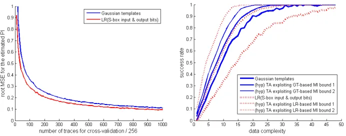
of the number of traces in the cross–validation set, e.g. by computing the square root of the Mean Square Error (MSE) for the PI based on these new estimates. The result of this experiment is given in the left part of Figure 8 (as an alter-native, we can also derive the quantiles of the estimated PI as in Appendix B, Figure 15). After 100 traces, the root MSE approximately equals 0.29 for the regression-based profiling. Our ideal expectation is that by summing the esti-mated PI obtained for LR-based profiling in Section 3 (≈0.38) with this value, we would obtain a “bound” on the MI of≈0.67. Of course, this bound would be probabilistic (i.e. with a certain chance that the information loss exceeds 0.29). A more confident bound would then be obtained by summing this root MSE twice, leading to an hypothetical MI of 0.96. Assuming the PI estimates to be Gaussian-distributed, the probability that the MI exceeds these bounds could also be quantified (to 31.8% and 4.6%, i.e. corresponding to the addition of one or two standard deviations to the mean of a normal distribution). The quantiles in Figure 15 lead to similar results (confirming the Gaussian assumption). Interpretation.Such an information theoretic evaluation would conclude that for leakage sample 2605 of our resistor-based measurements: (1) we identified a regression-based attack able to exploit a PI of ≈ 0.38; (2) we identified a template attack able to exploit a PI of≈0.58; (3) with some confidence, there may exist a stronger attack able to exploit an hypothetical MI of ≈0.67 (that would be identified with better assumptions); (4) with higher confidence, there may exist an even stronger attack able to exploit an hypothetical MI of≈0.96. Tighter “bounds” can be obtained by using our Gaussian templates, since we could not detect any assumption error in this case. That is, we would then expect that the assumption errors will be lower than the estimation errors on the PI with 256 000 traces in the cross–validation set. This would lead to MI bounds of
≈0.58 + 0.11 = 0.69 (with some confidence) and≈0.58 + 2×0.11 = 0.8 (with higher confidence). As mentioned in Section 2.2, these values of MI/PI can be used as predictors for the success rates of the corresponding attacks. Such success rates can be computed for the PI values and simulated for the hypothetical MI ones6, as represented in the right part of Figure 8. Note that this figure is only illustrative as the connection between the MI/PI and the success rates of attacks using the same models is not proved (in fact, there exists counter-examples [37]). But it was confirmed for many representative case studies7, and illustrates (1) how the MI/PI metrics translate into a number of traces to recover the key and (2) how better assumptions generally lead to tighter security guarantees. Can such bounds be accurate in general? Obtaining bounds on the infor-mation loss such as just described informally would be highly desirable. But it naturally requires a confirmation that such an approach can be independent of
6 The techniques in [26, 27] can be used for this purpose. Essentially, the evaluator will
use the (well estimated) means of the profiled models with additive Gaussian noise to simulate the traces. He will then adapt the noise level to reach the required MI value and use the corresponding simulated traces to compute success rates.
7
Fig. 8.Resistor-based measurements, sample 2605. Left: root MSE for the PI estimates obtained in Figure 1. Right: success rates of LR-based and Gaussian template attacks compared with hypothetical template attacks exploiting different MI bounds.
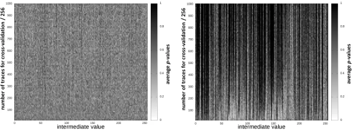
the distributions and statistical tools used for their estimation. Arguing about this issue once again faces the problem that the leakage PDF of cryptographic devices are generally unknown. Yet, one can use a simulated device for this pur-pose (i.e. a mathematical object for which we generate the leakages according to a known distribution, hence for which we know the MI). For example, we can analyze the MI and PI for a simulated device such that the leakage function deviates from the Hamming weight abstraction, while the evaluator still uses the Hamming weight function as leakage model. As a first step in this direction, we considered the model error as additive and Gaussian, and computed the MI, PI and three MI bounds, as illustrated in the left part of Figure 9. We see that for low noise levels, the true leakage model leads to 256 distinguishable events (i.e. MI=8) while the PI is stuck to≈2.5 (i.e. what can be extracted with a Hamming weight model). And as the noise increases, these 256 events first merge into 9 Hamming weight-like events, which then become hard to distinguish for standard deviations beyond 10−1. The bounds are given for three noise levels, for which the detection of assumption errors is given in the right part of the figure. Two different (negative) observations can be extracted from these experiments. First, many selection rules for the threshold value Nth
t could be defined (the figure uses average p-values), and none of the ones we considered provided accurate bounds independent of the noise level. For example, the bound for the standard deviation 10−4 does not capture the large MI-PI difference in our simulations. Second, any bound obtained from the MSE will anyway become pessimistic as the physical noise increases (since its impact will eventually dominate the one of assumption errors in the MSE). This is typically observed for the noise level 100 in Figure 9. As a result, we can conclude that precisely quantifying the informa-tion loss due to incorrect assumpinforma-tions in side-channel attacks is not possible with the techniques presented in this paper. Improving this situation is an interesting scope for further (theoretical) research. For example, one could try to establish selection rules forNth
contri-Fig. 9.Left: mutual information bounds for three noise standard deviations (simulated attacks). Right: detection of assumption errors for the same noise standard deviations.
butions of the physical noise and assumption errors in the MSE (but this would require to have more observations than sources [16], which may not always be the case, e.g. in power analysis). Yet, in practice these techniques would also drive us away from the goal of analyzing cryptographic devices independent of their leakage distributions. In the next section, we try to avoid such bottlenecks and conclude this paper by suggesting pragmatic guidelines for evaluators.
7
Pragmatic evaluation guidelines & conclusions
While measuring the information loss due to incorrect assumptions appears dif-ficult in general, the experiments of Figure 9 can also be concluded more pos-itively. Namely, they exhibit that as these errors are detected later, the MI-PI difference also decreases. So even if the intuition in the previous section cannot lead to quantitative bounds, it still leads to qualitatively interesting outcomes. In this respect, we believe the tools introduced in this work are essential for the fair evaluation of side-channel attacks, and should be exploited as follows.
the pragmatic question: “for an amount of measurements performed by a lab-oratory, is it worth spending time to refine the leakage model exploited in the evaluation?”. In other words, it can be used to guarantee that the security level suggested by a side-channel analysis is close to the worst-case, and this guarantee is indeed conditional to number of measurement available for this purpose.
Open problems can be envisioned in three main directions. First note that the most important contribution of this work is to put side-channel evaluations on solid foundations. The separation between estimation and assumption errors is fundamental in this respect. By contrast, the precise procedures we propose for their estimation, as well as the test for detecting incorrect models in Sec-tion 5, are first instances for this purpose. Alternative soluSec-tions could certainly be investigated (e.g. to obtain better confidence in the conclusions with less ef-forts), and constitute an interesting research topic. Besides, the application of the techniques described to more implementations (e.g. protected with counter-measures such as masking), for which the selection of relevant assumptions will be more difficult, is certainly worth further investigations as well. Eventually, the best combination of our tools with dimensionality reduction techniques (or any other preprocessing of the measurements), allowing to efficiently detect/exploit multiple points of interest in leakage traces, is another interesting question. Acknowledgements. This work has been funded in parts by the ERC project 280141 (acronym CRASH), the Walloon Region MIPSs project and the 7th framework European project PREMISE. Fran¸cois-Xavier Standaert is an asso-ciate researcher of the Belgian Fund for Scientific Research (FNRS-F.R.S.).
References
1. T. W. Anderson. On the distribution of the two-sample Cramer-von Mises criterion.
The Annals of Mathematical Statistics, 33(3):1148–1159, 1962.
2. Josep Balasch, Sebastian Faust, Benedikt Gierlichs, and Ingrid Verbauwhede. The-ory and practice of a leakage resilient masking scheme. In Wang and Sako [40], pages 758–775.
3. Robert Bartoszynski, Dennis K. Pearl, and John Lawrence. A multidimensional goodness-of-fit test based on interpoint distances.Journal of the American Statis-tical Association, 92(438):pp. 577–586, 1997.
4. Ali Galip Bayrak, Francesco Regazzoni, Philip Brisk, Fran¸cois-Xavier Standaert, and Paolo Ienne. A first step towards automatic application of power analysis countermeasures. In Leon Stok, Nikil D. Dutt, and Soha Hassoun, editors,DAC, pages 230–235. ACM, 2011.
5. Eric Brier, Christophe Clavier, and Francis Olivier. Correlation power analysis with a leakage model. In Marc Joye and Jean-Jacques Quisquater, editors,CHES, volume 3156 ofLNCS, pages 16–29. Springer, 2004.
6. Chakravarti, Laha, and Roy. Handbook of methods of applied statistics, Volume I, John Wiley and Sons, pp. 392-394, 1967.
7. Suresh Chari, Josyula R. Rao, and Pankaj Rohatgi. Template attacks. In Burton S. Kaliski Jr., C¸ etin Kaya Ko¸c, and Christof Paar, editors,CHES, volume 2523 of
LNCS, pages 13–28. Springer, 2002.
9. M. Abdelaziz Elaabid and Sylvain Guilley. Portability of templates. J. Crypto-graphic Engineering, 2(1):63–74, 2012.
10. Guillaume Fumaroli, Ange Martinelli, Emmanuel Prouff, and Matthieu Rivain. Affine masking against higher-order side channel analysis. In Alex Biryukov, Guang Gong, and Douglas R. Stinson, editors, Selected Areas in Cryptography, volume 6544 ofLNCS, pages 262–280. Springer, 2010.
11. S. Geisser. Predictive inference, volume 55. Chapman & Hall/CRC, 1993. 12. Louis Goubin and Ange Martinelli. Protecting AES with Shamir’s secret sharing
scheme. In Preneel and Takagi [22], pages 79–94.
13. Trevor Hastie, Robert Tibshirani, and Jerome Friedman.The elements of statistical learning. Springer Series in Statistics. Springer New York Inc., New York, NY, USA, 2001.
14. Jen-Fue Maa, Dennis K. Pearl, and Robert Bartoszynski. Reducing multidimen-sional two-sample data to one-dimenmultidimen-sional interpoint comparisons. The Annals of Statistics, 24(3):pp. 1069–1074, 1996.
15. Fran¸cois Mac´e, Fran¸cois-Xavier Standaert, and Jean-Jacques Quisquater. Infor-mation theoretic evaluation of side-channel resistant logic styles. In Pascal Paillier and Ingrid Verbauwhede, editors, CHES, volume 4727 of LNCS, pages 427–442. Springer, 2007.
16. David J. C. MacKay.Information theory, inference, and learning algorithms. Cam-bridge University Press, 2003.
17. Houssem Maghrebi, Claude Carlet, Sylvain Guilley, and Jean-Luc Danger. Optimal first-order masking with linear and non-linear bijections. In Aikaterini Mitrokotsa and Serge Vaudenay, editors,AFRICACRYPT, volume 7374 ofLNCS, pages 360– 377. Springer, 2012.
18. Houssem Maghrebi, Emmanuel Prouff, Sylvain Guilley, and Jean-Luc Danger. A first-order leak-free masking countermeasure. In Orr Dunkelman, editor,CT-RSA, volume 7178 ofLNCS, pages 156–170. Springer, 2012.
19. S. Mangard, E. Oswald, and F.-X. Standaert. One for all – all for one: Unifying standard differential power analysis attacks. IET Information Security, 5(2):100– 110, 2011.
20. Stefan Mangard. Hardware countermeasures against DPA ? A statistical analysis of their effectiveness. In Tatsuaki Okamoto, editor,CT-RSA, volume 2964 ofLNCS, pages 222–235. Springer, 2004.
21. Marcel Medwed and Fran¸cois-Xavier Standaert. Extractors against side-channel attacks: weak or strong? J. Cryptographic Engineering, 1(3):231–241, 2011. 22. Bart Preneel and Tsuyoshi Takagi, editors.Cryptographic Hardware and Embedded
Systems - CHES 2011 - 13th International Workshop, Nara, Japan, September 28 - October 1, 2011. Proceedings, volume 6917 ofLNCS. Springer, 2011.
23. Emmanuel Prouff and Thomas Roche. Attack on a higher-order masking of the AES based on homographic functions. In Guang Gong and Kishan Chand Gupta, editors,INDOCRYPT, volume 6498 ofLNCS, pages 262–281. Springer, 2010. 24. Ronald Pyke. Spacings revisited. In Proceedings of the Sixth Berkeley
Sympo-sium on Mathematical Statistics and Probability (Univ. California, Berkeley, Calif., 1970/1971), Vol. I: Theory of statistics, pages 417–427, Berkeley, Calif., 1972. Univ. California Press.
26. Mathieu Renauld, Dina Kamel, Fran¸cois-Xavier Standaert, and Denis Flandre. Information theoretic and security analysis of a 65-nanometer DDSLL AES S-box. In Preneel and Takagi [22], pages 223–239.
27. Mathieu Renauld, Fran¸cois-Xavier Standaert, Nicolas Veyrat-Charvillon, Dina Kamel, and Denis Flandre. A formal study of power variability issues and side-channel attacks for nanoscale devices. In Kenneth G. Paterson, editor, EURO-CRYPT, volume 6632 ofLNCS, pages 109–128. Springer, 2011.
28. Thomas Roche and Emmanuel Prouff. Higher-order glitch free implementation of the AES using secure multi-party computation protocols - extended version. J. Cryptographic Engineering, 2(2):111–127, 2012.
29. Werner Schindler, Kerstin Lemke, and Christof Paar. A stochastic model for dif-ferential side channel cryptanalysis. In Josyula R. Rao and Berk Sunar, editors,
CHES, volume 3659 ofLNCS, pages 30–46. Springer, 2005.
30. B.W. Silverman. Density estimation for statistics and data analysis. Monographs on Statistics and Applied Probability. Taylor & Francis, 1986.
31. Fran¸cois-Xavier Standaert and C´edric Archambeau. Using subspace-based tem-plate attacks to compare and combine power and electromagnetic information leakages. In Elisabeth Oswald and Pankaj Rohatgi, editors, CHES, volume 5154 ofLNCS, pages 411–425. Springer, 2008.
32. Fran¸cois-Xavier Standaert, Fran¸cois Koeune, and Werner Schindler. How to com-pare profiled side-channel attacks? In Michel Abdalla, David Pointcheval, Pierre-Alain Fouque, and Damien Vergnaud, editors,ACNS, volume 5536 ofLNCS, pages 485–498, 2009.
33. Fran¸cois-Xavier Standaert, Tal Malkin, and Moti Yung. A unified framework for the analysis of side-channel key recovery attacks. In Antoine Joux, editor, EURO-CRYPT, volume 5479 ofLNCS, pages 443–461. Springer, 2009.
34. Fran¸cois-Xavier Standaert, Eric Peeters, C´edric Archambeau, and Jean-Jacques Quisquater. Towards security limits in side-channel attacks. In Louis Goubin and Mitsuru Matsui, editors, CHES, volume 4249 of LNCS, pages 30–45. Springer, 2006.
35. Fran¸cois-Xavier Standaert, Christophe Petit, and Nicolas Veyrat-Charvillon. Masking with randomized look up tables - towards preventing side-channel at-tacks of all orders. In David Naccache, editor,Cryptography and Security, volume 6805 ofLNCS, pages 283–299. Springer, 2012.
36. Fran¸cois-Xavier Standaert, Nicolas Veyrat-Charvillon, Elisabeth Oswald, Benedikt Gierlichs, Marcel Medwed, Markus Kasper, and Stefan Mangard. The world is not enough: Another look on second-order DPA. In Masayuki Abe, editor, ASI-ACRYPT, volume 6477 ofLNCS, pages 112–129. Springer, 2010.
37. Francois-Xavier Standaert, Tal G. Malkin, and Moti Yung. A unified framework for the analysis of side-channel key recovery attacks (extended version). Cryptology ePrint Archive, Report 2006/139, 2006. http://eprint.iacr.org/.
38. Nicolas Veyrat-Charvillon, Marcel Medwed, St´ephanie Kerckhof, and Fran¸ cois-Xavier Standaert. Shuffling against side-channel attacks: A comprehensive study with cautionary note. In Wang and Sako [40], pages 740–757.
39. Nicolas Veyrat-Charvillon and Fran¸cois-Xavier Standaert. Generic side-channel distinguishers: Improvements and limitations. In Phillip Rogaway, editor,
CRYPTO, volume 6841 ofLNCS, pages 354–372. Springer, 2011.
A
Histograms and kernels
B
Additional figures
Fig. 10.Resistor-based measurements.
Fig. 12.Electromagnetic measurements.
Fig. 14. PI for univariate and multivariate leakage models. Left: two points (2605, 4978) coming from the resistor-based measurements. Right: multi-channel attack ex-ploiting the same point (2605) from resistor- and inductance-based measurements.