Leptoquarks in Flavour Physics

(1)

c

Owned by the authors, published by EDP Sciences, 2018

ZU-TH 39/

Leptoquarks in Flavour Physics

Dario Müller1,2,a

1_{Paul Scherrer Institut, CH–5232 Villigen PSI, Switzerland}

2_{Physik Institut, Universität Zürich, Winterthurstrasse 190,CH-8057 Zürich, Switzerland}

Abstract.While the LHC has not directly observed any new particle so far, experimental results from LHCb, BELLE and BABAR point towards the violation of lepton flavour universality inb→s+−_and_b_→_c_ν_{. In} this context, also the discrepancy in the anomalous magnetic moment of the muon can be interpreted as a sign of lepton flavour universality violation. Here we discuss how these hints for new physics can also be explained by introducing leptoquarks as an extension of the Standard Model. Indeed, leptoquarks are good candidates to explain the anomaly in the anomalous magnetic moment of the muon because of anmt/mµenhanced

contribu-tion giving correlated effects inZboson decays which is particularly interesting in the light of future precision experiments.

1 Introduction

So far the LHC has not directly observed any particles be-yond the ones in the Standard Model of particle physics (SM). While in the SM the Higgs boson couplings to fermions are the only source of lepton flavour universal-ity violation (LFUV), in the past years several hints for additional LFUV have been accumulated. The ratios of semi-leptonicBdecays

RK(∗)₌_Br_B_→_K(∗)_µ+_µ₋ _Br_B

→K(∗)_e+_e₋_,

RD(∗)₌_Br_B_→_D(∗)_τν _Br_B_→_D(∗)_ν_,

RJ/Ψ

=Br

B+

c →J/Ψτ+ν

BrBc→J/Ψµ+ν

,

show sizeable deviations from the SM predictions. Consideringb→s+−_transitions,_R₍_K_{) [1] and}_R₍_K∗_{) [2]} show a combined significance for LFUV at the 4σ level [3–7]. If we also take into account all other b →

sµ+_µ− _{observables, in several scenarios the global fit} prefers new physics (NP) above the 5σlevel [8].

InR(D(∗)_{) BaBar [9], BELLE [10, 11] and LHCb [12, 13]} found a significance for LFUV of about 4σ[14]. In this context it is interesting to mention that LHCb recently measured a deviation of about 2σinR(J/Ψ) [15]. This is consistent with the anomaly inR(D) andR(D∗_). The tension in the anomalous magnetic moment of the muon (aµ) between measurement [16] and SM prediction is at the 3σlevel [17, 18]. Also this discrepancy can be interpreted as a sign of LFUV even though the anoma-lous magnetic moments are already in the SM flavour non-universal: If we assume that NP coupled with the same

a_{e-mail: [email protected]}

strength to electrons and to muons,aewould be more

sen-sitive for NP. Since no deviation from the SM prediction inaehas been observed so far, the tension inaµcan be in-terpreted as another sign for LFUV induced by NP. Motivated by these anomalies, we study leptoquarks (LQ) which provide a possible solution of them. Firstly we con-centrate on each anomaly itself and discuss which LQ rep-resentations suit best for an explanation and consider cor-related effects in other observables. Finally, we will inves-tigate if we can explain the described anomalies simulta-neously.

2 a

µ

In order to explain the descrepancy inaµ, a rather large ef-fect of the order of the SM weak interaction contribution is required. Among the set of new particles that can give the desired effect, LQ are interesting candidates [19–23]. Even though the LQ must be rather heavy due to LHC con-straints (above 1 TeV), one can still get relevant effects in

aµ. For some representations of LQ, the amplitude can be enhanced by a factormt/mµ O(103) ormb/mµ O(10) compared to the SM.

To achieve an enhancement of factormt/mµ, the LQ must couple to left- and right-handed top or anti-top quarks si-multaneously. However, not all LQ representations have this feature. Among the 10 scalar and vector LQ represen-tations generating lepton-quark interaction terms that are invariant under the SM gauge group [24], only two scalars can possess this enhancement: An SU(2) singletΦ₁ and an SU(2) doubletΦ₂with quantum numbers

QΦ₁:

3,1,−2₃

, Q(Φ2) :

¯3,2,−7₃

(2)

µ− _µ− Φ−5/3

Φ−1/3

t(tc₎

γ mt

Z0

ℓ− f

ℓ+ i Φ−5/3

Φ−1/3

t(tc₎

mt

Figure 1.Feynman diagrams that contribute toaµandZ→i+−f. The crosses on the fermion lines stand for chirality flips, involving a top mass.

These representations couple to the fermions of the SM as follows

Lint =λ1_{f i}Ruc

fi+λ1f iLQcfiτ2Li

Φ†₁, (2)

Lint =λ2_{f i}RLufLi+λ2_{f i}LRQfiτ2iΦ†₂. (3)

QandLare SU(2) doublets,uandare SU(2) singlets and

cdenotes charge conjugation. f andiare flavour indices. The Feynman diagrams involving Φ₁ andΦ₂ are shown left in Fig. 1.

For simplicity, we only consider couplings of top quarks to muons and setλ1₃₂L,1Randλ₃₂2RL,2LRequal toλLµ,R. Besides the contribution toaµ, we also obtain correlated effects in

Z → µ+_µ−_{(see the right Feynman diagram in Fig. 1), in} b → sν¯ν (for Φ₁) and inb → sµ+_µ− _(for _Φ₂_{). Fig. 2} shows the allowed regions inλLµ-λRµparameter space for a LQ with mass of 1 TeV, to respect constraints from direct searches. ForZ →µ+_µ−_{the expected bounds from GigaZ} [25] and TLEP [26] are shown as well. Additionally, for Φ1 the expected BELLE II limit forB→ K(∗)ν¯νis taken into account. Φ2 gives a C9 = C10-like contribution to b→s+−_{which provides a slight improvement of 1}_σ_in the global fit.

If we also allow for couplings of the top quark to taus or electrons, lepton flavour violating processes asτ_→µγor

Z → µewill be possible. A more detailed discussion can be found in Ref. [27].

3 b

_→

s

+

−

Dealing with b → s+₋ _{transitions, one usually works}

with an effective Hamiltonian of the form

Hfi eff =−

4GF

√ 2VtbV

∗

ts

a=9,10

Caf iOaf i+Caf iOaf i, (4)

O₉₍₁₀₎f i = α 4π[ ¯sγ

µ_P

Lb] [¯fγµ(γ5)i], (5)

O₉₍₁₀₎f i = α

4π[ ¯sγµPRb] [¯fγµ(γ5)i]. (6)

Then, for several scenarios with NP inC9only,C9=−C10 or C9 = −C₉, the global fit prefers NP above the 5σ level [8].

We consider the case where NP contributes asC9=−C10.

While in the muon channel the preferred value deviates from the SM prediction with a tension of 5σ, in the case with electrons the SM contribution is sufficient to give a good fit to the data. To reach the central value, anO(10%) NP effect in the muon channel is required. b _→ s+− is suppressed by a loop and a CKM factor because it is a flavour changing neutral current. Therefore, the effect of NP does not have to be very large to account for the data. There are several suggestions to explain the anomaly in

b→sµ+_µ−_{with LQ, see e.g. [28–41].}

There are three LQ representations that give aC9 =−C10 -like contribution tob→s+−

Φ₃:

3,3,−2₃

, _Lint=λ3f iQcfiτ2(τ·Φ3)†Li, (7)

Vµ

1 :

¯3,1,−4₃

, _Lint=κ1_{f i}Rdfγµi+κ1_{f i}LQfγµLiV₁µ†,

(8)

Vµ

3 :

3,3,4 3

, Lint=κ3f iQfγµ

τ·Vµ

3

Li. (9)

If we only allow for couplings to muons, these LQ will give tree-level effects inb→ sµ+_µ−_{but contribute at} loop-level in other flavour observables. This is why LQ can explain the anomalies inb→ sµ+_µ−_{transitions but are not} in conflict with other observables.

Including couplings to electrons, we get additional effects in b → se+_e− _{as well as in the lepton flavour violating} processesµ_→eγandb→ sµe. We can write

Brµ→eγ∝χCee₉ +C µµ

9 χ 2

, (10)

BrB→Kµe∝C

ee 9 γ 2

+γCµµ

9 2

, (11)

whereχ=y32/y21andγ=y21/y22, withy=λfor scalar LQ andy = κfor vector LQ. Note that one can avoid an effect inµ → eγcompletely ifCµµ₉ = −χ2Cee₉. For real values of χ this means that sign[Cee

9 ] = −sign[C

µµ

9 ]. In Fig. 3 you find a detailed analysis for the scalar tripletΦ3. ForVµ

1 andV

µ

(3)

µ− _µ− Φ−5/3

Φ−1/3

t(tc₎

γ mt

Z0

ℓ− f

ℓ+ i Φ−5/3

Φ−1/3

t(tc₎

mt

Figure 1.Feynman diagrams that contribute toaµandZ→i+−f. The crosses on the fermion lines stand for chirality flips, involving a top mass.

These representations couple to the fermions of the SM as follows

Lint=λ1_{f i}Ruc

fi+λ1f iLQcfiτ2Li

Φ†₁, (2)

Lint=λ2_{f i}RLufLi+λ2_{f i}LRQfiτ2iΦ†₂. (3)

QandLare SU(2) doublets,uandare SU(2) singlets and

cdenotes charge conjugation. f andiare flavour indices. The Feynman diagrams involving Φ₁ andΦ₂ are shown left in Fig. 1.

For simplicity, we only consider couplings of top quarks to muons and setλ1₃₂L,1Randλ₃₂2RL,2LRequal toλLµ,R. Besides the contribution toaµ, we also obtain correlated effects in

Z → µ+_µ−_{(see the right Feynman diagram in Fig. 1), in} b → sν¯ν (for Φ₁) and inb → sµ+_µ− _(for _Φ₂_{). Fig. 2} shows the allowed regions inλµL-λRµparameter space for a LQ with mass of 1 TeV, to respect constraints from direct searches. ForZ→µ+_µ−_{the expected bounds from GigaZ} [25] and TLEP [26] are shown as well. Additionally, for Φ1 the expected BELLE II limit forB → K(∗)ν¯νis taken into account. Φ2 gives a C9 = C10-like contribution to b→s+−_{which provides a slight improvement of 1}_σ_in the global fit.

If we also allow for couplings of the top quark to taus or electrons, lepton flavour violating processes asτ_→µγor

Z → µewill be possible. A more detailed discussion can be found in Ref. [27].

3 b

_→

s

+

−

Dealing with b → s+₋ _{transitions, one usually works}

with an effective Hamiltonian of the form

Hfi eff =−

4GF

√ 2VtbV

∗

ts

a=9,10

Caf iOaf i+Caf iOaf i, (4)

O₉₍₁₀₎f i = α 4π[ ¯sγ

µ_P

Lb] [¯fγµ(γ5)i], (5)

O₉₍₁₀₎f i = α

4π[ ¯sγµPRb] [¯fγµ(γ5)i]. (6)

Then, for several scenarios with NP inC9only,C9=−C10 or C9 = −C₉, the global fit prefers NP above the 5σ level [8].

We consider the case where NP contributes asC9 =−C10.

While in the muon channel the preferred value deviates from the SM prediction with a tension of 5σ, in the case with electrons the SM contribution is sufficient to give a good fit to the data. To reach the central value, anO(10%) NP effect in the muon channel is required. b _→ s+− is suppressed by a loop and a CKM factor because it is a flavour changing neutral current. Therefore, the effect of NP does not have to be very large to account for the data. There are several suggestions to explain the anomaly in

b→sµ+_µ−_{with LQ, see e.g. [28–41].}

There are three LQ representations that give aC9=−C10 -like contribution tob→s+−

Φ₃ :

3,3,−2₃

, _Lint =λ3f iQcfiτ2(τ·Φ3)†Li, (7)

Vµ

1 :

¯3,1,−4₃

, _Lint =κ1_{f i}Rdfγµi+κ1_{f i}LQfγµLiV₁µ†,

(8)

Vµ

3 :

3,3,4 3

, Lint=κ3f iQfγµ

τ·Vµ

3

Li. (9)

If we only allow for couplings to muons, these LQ will give tree-level effects inb→sµ+_µ−_{but contribute at} loop-level in other flavour observables. This is why LQ can explain the anomalies inb→ sµ+_µ−_{transitions but are not} in conflict with other observables.

Including couplings to electrons, we get additional effects in b → se+_e− _{as well as in the lepton flavour violating} processesµ_→eγandb→ sµe. We can write

Brµ→eγ∝χCee₉ +C µµ 9 χ 2 , (10)

BrB→Kµe∝C

ee 9 γ 2

+γCµµ

9 2

, (11)

whereχ=y32/y21andγ=y21/y22, withy=λfor scalar LQ andy = κfor vector LQ. Note that one can avoid an effect inµ → eγcompletely ifCµµ₉ = −χ2Cee₉. For real values of χ this means that sign[Cee

9 ] = −sign[C

µµ

9 ]. In Fig. 3 you find a detailed analysis for the scalar tripletΦ3. ForVµ

1 andV

µ

3 the situation is quite similar, albeit the blue bands are more narrow. For more information see Ref. [42].

-1.5 -1.0 -0.5 0.0 0.5 1.0 1.5

-1.5 -1.0 -0.5 0.0 0.5 1.0 1.5 L R

BK*

BK*(BELLE II) Z(LEP)

Z(GigaZ)

Z(TLEP)

a(2) bs

-0.6 -0.4 -0.2 0.0 0.2 0.4 0.6 -0.6 -0.4 -0.2 0.0 0.2 0.4 0.6

λμL λμ

R

Figure 2.Allowed regions in theλµL-λRµparameter space from current limits of LEP and expected future constraints of GigaZ and TLEP

withMLQ=1 TeV. Left: SU(2) singletΦ1. Right: SU(2) doubletΦ2. Note that if the expected sensitivity of TLEP was reached and no

excess in theZµµ¯-coupling was found, an explanation of the anomaly inaµwould strongly be disfavoured.

4 b

_→

c

τν

The transitionb → cτνis a charged current process and is therefore generated at tree-level in the SM. Since an explanation of R(D) and R(D∗_{) requires an} _O_(10%) ef-fect, also the NP must contribute at tree-level. Charged Higgses [44–48], W _{bosons [31] and LQ [22, 23, 32,} 33, 35, 49, 49–54] are NP candidates. However,Bc

life-time [55, 56] andq2_{distributions [57] in combination with} direct searches [58] strongly disfavour charged Higgses andW_bosons.

Hence, we are left with LQ. If we want to explain the ex-cess inR(D) andR(D∗_{) by modifying the couplings to tau} neutrinos and/or taus, we also get effects in b → sτ+_τ− andb → sν¯ν. It can be shown in a model independent way that these effects are of the order of 103 compared to the SM [33]. This is due to the fact that the processes

b → sτ+_τ−_and_b _→ _s_ν¯_ν_{occur at loop-level in the SM,} while LQ contribute at tree-level with considerably large couplings in order to explainR(D(∗)_{). An}_O₍₁₀3_{) e}_ff_{ect is} in strong conflict with experimental results ofB→K(∗)_ν¯_ν. Hence, a model that explainsR(D) andR(D∗_{) must avoid} a major effect inb → sν¯ν. One possibility is the vector LQ singlet Vµ

1 (see Eq. (8)). Another model was pro-posed in Ref. [59], where instead of Vµ

1 two scalar LQ (the SU(2) singletΦ₁in Eq. (2) and the SU(2) tripletΦ₃ in Eq. (7)) are required. If Fig. 4 we can see for which parameters we can explain R(D(∗)_{) without violating the} limits ofb→sν¯ν.

Besides explainingR(D(∗)_{), it also enhances}_B_s _→ _τ+_τ− up to a factor 103 _{compared to the SM and therefore} lies within experimental reach. The current limit is BrBs→τ+τ−<6.8×10−3[60]. Fig. 5 shows the

corre-lation ofR(D(∗)_{) and Br}_B

s→τ+τ−.

5 Simultaneous Explanation

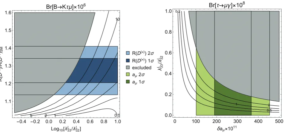
We may ask if one can explain the three types of anoma-lies inaµ,b→sµ+µ−andR(D(∗)) simultaneously. If we take the model that we proposed in Sec. 4 and insert a discrete symmetry for the couplingsλ1_jkL =eiπjλ3_jk_≡λL_jk the effect in b _→ sν¯νwill be cancelled exactly. If we include b → sµ+_µ−_, _B _→ _D(∗)_µν/_B _→ _D(∗)_e_ν _{will be} affected. However, these observables remain compatible with experiments. Additionally the LFV processτ→ µγ andb → sτµappear. Both processes give constraints on our parameter space. On the left-hand side of Fig. 6 the allowed regions for MLQ = 1 TeV are shown, under the

assumption thatb → sµ+_µ₋_{matches the central value of}

the global fit. As we can see easily, the explanation of

R(D(∗)_{) requires} _λL

33/λL32 > 1. On the right-hand side of Fig. 6 we needλL₃₃/λL₃₂<0.6 to explainaµwithout getting in conflict with experimental constraints ofτ_→µγ. With this contradiction, we cannot explain all three anomalies simultaneously. However, if we abandon anyone of them, it is possible to explain the other two anomalies. If we abandon the assumptionλ1_jkL = eiπjλ3_jkone can avoid the discussed constraints and explain all three anomalies. Another good candidate is the vector LQ singlet Vµ

1 be-cause it does not affect theb→sν¯νtransitions but gives a

C9 =−C10effect inb→ s+−. It can also be used to ex-plainR(D(∗)_{). In}_a

µwe can obtain anmb/mµcontribution which is not as large as for the two scalar LQΦ₁ andΦ₂ (see Sec.2), but still may be significant.

(4)

phe--1.0 -0.5 0.0 0.5 1.0

-1.0

-0.5 0.0 0.5 1.0

C

₉

=-

C

₁₀

C

9

ee

=-C

10

ee

=1

=4

=0.25

Br[ e] <5.7·10-13_{Scalar Triplet}

bs+-₍₁₎

bs+-₍₂₎

Br[BK±e]·108with=1

Figure 3.The darker (lighter) red region shows the global fit at 1σ(2σ) forb→se+_e−_and_b_→_s_µ+_µ−_{transitions. In blue, the allowed} region constrained by the current limit Brµ→eγ<4.2×10−13_{[43] with}_χ₌_{₁_/₄_,₁_,₄_}_{for the scalar triplet}_Φ

3withMLQ=1TeV. The outer (inner) green contour shows the case where BrB→Kµe=2_×10−8(0.2×10−8_{). For real values of}_χ_{only the region with}

Cµµ

9 <0 andCee9 >0 seems to be compatible with experimental limits. Indeed this is also where the central value of the global fit lies.

However, if in the future the global fit prefersCµµ

9 <0 andCee9 <0, LQ with real couplings will not be able to explainb→ s+−

transitions without violating the constraints fromµ_→eγ.

-0.6 -0.4 -0.2 0.0 0.2 0.4 0.6

sign[231L331L] 231L331L/M1[1/TeV]

sign

[

23

3

33

3]

23

3

33

3

/

M3

[

1

/

Te

V

]

R(D(*))2

R(D(*))1

bsallowed

Figure 4.In lighter (darker) blue you see the 1σ(2σ) preferred

region of the weighted sum ofR(D) andR(D∗_{), in yellow the} allowed region ofb→sνν¯.M1(3)is the mass of the LQΦ1(Φ3).

nomenologically consistent and leads to a massive vector LQ. This vector LQ has the properties ofVµ

1 in Eq. (8).

6 Conclusion

In these proceedings we reviewed which LQ are good can-didates to explain flavour anomalies: For the deviation in

aµthe scalar LQΦ1andΦ2give anmt/mµenhanced con-tribution. This is a useful feature to explain the rather large

1.0 1.2 1.4 1.6

0.000 0.002 0.004 0.006 0.008

R(D(*))/R(D(*))_SM

Br

[

Bs

]

R(D(*))2

R(D(*))1

Bsexcluded

Bs

Figure 5. In blue we have the weighted sum of R(D) and R(D∗_{) and the red line depicts the correlated prediction of} Br [Bs→τ+τ−]. The grey region shows the current experimental

bounds.

discrepancy. Consideringb→ s+₋_{transitions, the three}

LQ representationsΦ₃,V₁µandV₃µare required by the fit, because they giveC9=−C10.R(D(∗)) can be explained ei-ther byVµ

(5)

-1.0 -0.5 0.0 0.5 1.0

-1.0

-0.5 0.0 0.5 1.0

C

₉

=-

C

₁₀

C

9

ee

=-C

10

ee

=1

=4

=0.25

Br[ e] <5.7·10-13_{Scalar Triplet}

bs+-₍₁₎

bs+-₍₂₎

Br[BK±e]·108with=1

Figure 3.The darker (lighter) red region shows the global fit at 1σ(2σ) forb→se+_e−_and_b_→_s_µ+_µ−_{transitions. In blue, the allowed} region constrained by the current limit Brµ→eγ<4.2×10−13_{[43] with}_χ₌_{₁_/₄_,₁_,₄_}_{for the scalar triplet}_Φ

3withMLQ=1TeV. The outer (inner) green contour shows the case where BrB→Kµe=2_×10−8(0.2×10−8_{). For real values of}_χ_{only the region with}

Cµµ

9 <0 andCee9 >0 seems to be compatible with experimental limits. Indeed this is also where the central value of the global fit lies.

However, if in the future the global fit prefersCµµ

9 <0 andCee9 <0, LQ with real couplings will not be able to explainb→ s+−

transitions without violating the constraints fromµ_→eγ.

-0.6 -0.4 -0.2 0.0 0.2 0.4 0.6

sign[231L331L] 231L331L/M1[1/TeV]

sign

[

23

3

33

3]

23

3

33

3

/

M3

[

1

/

Te

V

]

R(D(*))2

R(D(*))1

bsallowed

Figure 4.In lighter (darker) blue you see the 1σ(2σ) preferred

region of the weighted sum ofR(D) andR(D∗_{), in yellow the} allowed region ofb→sνν¯. M1(3)is the mass of the LQΦ1(Φ3).

nomenologically consistent and leads to a massive vector LQ. This vector LQ has the properties ofVµ

1 in Eq. (8).

6 Conclusion

In these proceedings we reviewed which LQ are good can-didates to explain flavour anomalies: For the deviation in

aµthe scalar LQΦ1andΦ2give anmt/mµenhanced con-tribution. This is a useful feature to explain the rather large

1.0 1.2 1.4 1.6

0.000 0.002 0.004 0.006 0.008

R(D(*))/R(D(*))_SM

Br

[

Bs

]

R(D(*))2

R(D(*))1

Bsexcluded

Bs

Figure 5. In blue we have the weighted sum of R(D) and R(D∗_{) and the red line depicts the correlated prediction of} Br [Bs→τ+τ−]. The grey region shows the current experimental

bounds.

discrepancy. Consideringb→ s+₋_{transitions, the three}

LQ representationsΦ₃,V₁µandV₃µare required by the fit, because they giveC9=−C10.R(D(∗)) can be explained ei-ther byVµ

1 or, as we proposed, by a combination of a scalar LQ singletΦ1and scalar LQ tripletΦ3without getting in conflict withb → sν¯νobservables. We also showed that this model is able to explain any two of the three anomalies (aµ,b→ sµ+µ−andR(D(∗)) simultaneously.

0.5 1

2 5

10

-0.4 -0.2 0.0 0.2 0.4 0.6 0.8 1.0

1.1 1.2 1.3 1.4 1.5 1.6

Log10[33L/32L ]

R

(

D

(*))/

R

(

D

(*))

SM

Br[BK]×106

R(D(*))2

R(D(*))1

excluded

a2

a1

0.2

0.5

1 2

0 100 200 300 400 500

0.0 0.2 0.4 0.6 0.8 1.0

a×1011

33

L/

32

L

Br[]×108

Figure 6.Left: In blue we have the weighted sum ofR(D) andR(D∗_{). The contour lines show Br}_B_→_K_τµ_×₁₀6_{. Right: The anomaly}

inaµcombined with the contour lines depicting Brτ→µγ×108. In both plots the grey region is excluded by experiments.

Acknowledgments

D.M. thanks the organizing committee, and especially Gi-ancarlo D’Ambrosio, for the invitation and for giving the opportunity to present his work.

D.M. is supported by an Ambizione Grant of the Swiss National Science Foundation (PZ00P2_154834).

References

[1] R. Aaij et al. [LHCb Collaboration], Phys. Rev. Lett. 113 (2014) 151601 doi:10.1103/PhysRevLett.113.151601

[arXiv:1406.6482 [hep-ex]].

[2] R. Aaij et al. [LHCb Collaboration], JHEP

1708 (2017) 055 doi:10.1007/JHEP08(2017)055 [arXiv:1705.05802 [hep-ex]].

[3] W. Altmannshofer, P. Stangl and D. M. Straub, Phys. Rev. D 96 (2017) no.5, 055008 doi:10.1103/PhysRevD.96.055008 [arXiv:1704.05435 [hep-ph]].

[4] G. D’Amico, M. Nardecchia, P. Panci, F. Sannino, A. Strumia, R. Torre and A. Urbano, JHEP1709(2017) 010 doi:10.1007/JHEP09(2017)010 [arXiv:1704.05438 [hep-ph]].

[5] G. Hiller and I. Nisandzic, Phys. Rev. D 96 (2017) no.3, 035003 doi:10.1103/PhysRevD.96.035003 [arXiv:1704.05444 [hep-ph]].

[6] L. S. Geng, B. Grinstein, S. Jäger, J. Martin Camalich, X. L. Ren and R. X. Shi, Phys. Rev. D 96 (2017) no.9, 093006 doi:10.1103/PhysRevD.96.093006 [arXiv:1704.05446 [hep-ph]].

[7] T. Hurth, F. Mahmoudi, D. Martinez Santos and S. Neshatpour, Phys. Rev. D 96(2017) no.9, 095034

doi:10.1103/PhysRevD.96.095034 [arXiv:1705.06274 [hep-ph]].

[8] B. Capdevila, A. Crivellin, S. Descotes-Genon, J. Ma-tias and J. Virto, arXiv:1704.05340 [hep-ph].

[9] J. P. Lees et al. [BaBar Collabo-ration], Phys. Rev. Lett. 109 (2012) 101802 doi:10.1103/PhysRevLett.109.101802 [arXiv:1205.5442 [hep-ex]].

[10] M. Huschle et al. [Belle Collabora-tion], Phys. Rev. D 92 (2015) no.7, 072014 doi:10.1103/PhysRevD.92.072014 [arXiv:1507.03233 [hep-ex]].

[11] S. Hirose et al. [Belle Collaboration], arXiv:1709.00129 [hep-ex].

[12] R. Aaij et al. [LHCb Collaboration], Phys. Rev. Lett. 115 (2015) no.11, 111803 Erratum: [Phys. Rev. Lett. 115 (2015) no.15, 159901] doi:10.1103/PhysRevLett.115.159901, 10.1103/ Phys-RevLett.115.111803 [arXiv:1506.08614 [hep-ex]]. [13] F. Betti [LHCb Collaboration], arXiv:1705.10651

[hep-ex].

[14] Y. Amhiset al., arXiv:1612.07233 [hep-ex].

[15] R. Aaij et al. [LHCb Collaboration], arXiv:1711.05623 [hep-ex].

[16] G. W. Bennett et al. [Muon g-2 Collab-oration], Phys. Rev. D 73 (2006) 072003 doi:10.1103/PhysRevD.73.072003 [hep-ex/0602035]. [17] A. Nyffeler, Phys. Rev. D 94 (2016) no.5, 053006

doi:10.1103/PhysRevD.94.053006 [arXiv:1602.03398 [hep-ph]].

[18] F. Jegerlehner and A. Nyffeler, Phys. Rept.

(6)

[19] A. Djouadi, T. Kohler, M. Spira and J. Tutas, Z. Phys. C46(1990) 679. doi:10.1007/BF01560270

[20] S. Davidson, D. C. Bailey and B. A. Campbell, Z. Phys. C61(1994) 613 doi:10.1007/BF01552629 [hep-ph/9309310].

[21] G. Couture and H. Konig, Phys. Rev. D53 (1996) 555 doi:10.1103/PhysRevD.53.555 [hep-ph/9507263]. [22] M. Bauer and M. Neubert, Phys.

Rev. Lett. 116 (2016) no.14, 141802 doi:10.1103/PhysRevLett.116.141802

[arXiv:1511.01900 [hep-ph]].

[23] D. Das, C. Hati, G. Kumar and N. Ma-hajan, Phys. Rev. D 94 (2016) 055034 doi:10.1103/PhysRevD.94.055034 [arXiv:1605.06313 [hep-ph]].

[24] W. Buchmuller, R. Ruckl and D. Wyler, Phys. Lett. B 191 (1987) 442 Erratum: [Phys. Lett. B

448 (1999) 320]. doi:10.1016/ S0370-2693(99)00014-3, 10.1016/0370-2693(87)90637-X

[25] H. Baeret al., arXiv:1306.6352 [hep-ph].

[26] M. Bicer et al. [TLEP Design Study Working Group], JHEP 1401 (2014) 164 doi:10.1007/JHEP01(2014)164 [arXiv:1308.6176 [hep-ex]].

[27] E. Coluccio Leskow, G. D’Ambrosio, A. Crivellin and D. Müller, Phys. Rev. D 95 (2017) no.5, 055018 doi:10.1103/PhysRevD.95.055018 [arXiv:1612.06858 [hep-ph]].

[28] B. Gripaios, M. Nardecchia and S. A. Renner, JHEP1505(2015) 006 doi:10.1007/JHEP05(2015)006 [arXiv:1412.1791 [hep-ph]].

[29] S. Fajfer and N. Košnik, Phys. Lett. B755(2016) 270 doi:10.1016/j.physletb.2016.02.018 [arXiv:1511.06024 [hep-ph]].

[30] D. Beˇcirevi´c, S. Fajfer and N. Košnik, Phys. Rev. D 92 (2015) no.1, 014016 doi:10.1103/PhysRevD.92.014016 [arXiv:1503.09024 [hep-ph]].

[31] A. Greljo, G. Isidori and D. Marzocca, JHEP

1507 (2015) 142 doi:10.1007/JHEP07(2015)142 [arXiv:1506.01705 [hep-ph]].

[32] L. Calibbi, A. Crivellin and T. Ota, Phys. Rev. Lett. 115 (2015) 181801 doi:10.1103/PhysRevLett.115.181801

[arXiv:1506.02661 [hep-ph]].

[33] R. Alonso, B. Grinstein and J. Martin Camalich, JHEP1510(2015) 184 doi:10.1007/JHEP10(2015)184 [arXiv:1505.05164 [hep-ph]].

[34] R. Barbieri, G. Isidori, A. Pattori and F. Senia, Eur. Phys. J. C76(2016) no.2, 67 doi:10.1140/epjc/ s10052-016-3905-3 [arXiv:1512.01560 [hep-ph]].

[35] D. Beˇcirevi´c, S. Fajfer, N. Košnik and O. Sumen-sari, Phys. Rev. D 94 (2016) no.11, 115021 doi:10.1103/PhysRevD.94.115021 [arXiv:1608.08501 [hep-ph]].

[36] D. Beˇcirevi´c, N. Košnik, O. Sumensari and R. Zukanovich Funchal, JHEP 1611 (2016) 035 doi:10.1007/JHEP11(2016)035 [arXiv:1608.07583

[hep-ph]].

[37] D. Beˇcirevi´c and O. Sumensari, JHEP1708(2017) 104 doi:10.1007/JHEP08(2017)104 [arXiv:1704.05835 [hep-ph]].

[38] D. Aloni, A. Dery, C. Frugiuele and Y. Nir, JHEP1711(2017) 109 doi:10.1007/JHEP11(2017)109 [arXiv:1708.06161 [hep-ph]].

[39] B. Chauhan, B. Kindra and A. Narang, arXiv:1706.04598 [hep-ph].

[40] O. Sumensari, arXiv:1705.07591 [hep-ph].

[41] C. H. Chen, T. Nomura and H. Okada, Phys. Lett. B774 (2017) 456 doi:10.1016/j.physletb.2017.10.005 [arXiv:1703.03251 [hep-ph]].

[42] A. Crivellin, D. Mueller, A. Signer and Y. Ulrich, arXiv:1706.08511 [hep-ph].

[43] A. M. Baldiniet al.[MEG Collaboration], Eur. Phys. J. C76(2016) no.8, 434 doi:10.1140/epjc/ s10052-016-4271-x [arXiv:1605.05081 [hep-ex]].

[44] A. Crivellin, C. Greub and A. Kokulu, Phys. Rev. D86(2012) 054014 doi:10.1103/PhysRevD.86.054014 [arXiv:1206.2634 [hep-ph]].

[45] M. Tanaka and R. Watanabe, Phys. Rev. D87(2013) no.3, 034028 doi:10.1103/PhysRevD.87.034028 [arXiv:1212.1878 [hep-ph]].

[46] A. Celis, M. Jung, X. Q. Li and A. Pich, JHEP1301(2013) 054 doi:10.1007/JHEP01(2013)054 [arXiv:1210.8443 [hep-ph]].

[47] A. Crivellin, A. Kokulu and C. Greub, Phys. Rev. D 87 (2013) no.9, 094031 doi:10.1103/PhysRevD.87.094031 [arXiv:1303.5877 [hep-ph]].

[48] A. Crivellin, J. Heeck and P. Stof-fer, Phys. Rev. Lett. 116 (2016) no.8, 081801 doi:10.1103/PhysRevLett.116.081801 [arXiv:1507.07567 [hep-ph]].

[49] R. Barbieri, C. W. Murphy and F. Senia, Eur. Phys. J. C77 (2017) no.1, 8 doi:10.1140/epjc/ s10052-016-4578-7 [arXiv:1611.04930 [hep-ph]].

[50] B. Chauhan and B. Kindra, arXiv:1709.09989 [hep-ph].

[51] I. Doršner, S. Fajfer, D. A. Faroughy and N. Košnik, JHEP1710(2017) 188 doi:10.1007/JHEP10(2017)188 [arXiv:1706.07779 [hep-ph]].

[52] O. Popov and G. A. White, Nucl. Phys. B

923 (2017) 324 doi:10.1016/j.nuclphysb.2017.08.007 [arXiv:1611.04566 [hep-ph]].

[53] G. Hiller, D. Loose and K. Schönwald, JHEP

[54] S. Sahoo, R. Mohanta and A. K. Giri, Phys. Rev. D 95 (2017) no.3, 035027 doi:10.1103/PhysRevD.95.035027 [arXiv:1609.04367 [hep-ph]].

(7)

[19] A. Djouadi, T. Kohler, M. Spira and J. Tutas, Z. Phys. C46(1990) 679. doi:10.1007/BF01560270

[20] S. Davidson, D. C. Bailey and B. A. Campbell, Z. Phys. C61(1994) 613 doi:10.1007/BF01552629 [hep-ph/9309310].

[21] G. Couture and H. Konig, Phys. Rev. D53 (1996) 555 doi:10.1103/PhysRevD.53.555 [hep-ph/9507263]. [22] M. Bauer and M. Neubert, Phys.

Rev. Lett. 116 (2016) no.14, 141802 doi:10.1103/PhysRevLett.116.141802

[arXiv:1511.01900 [hep-ph]].

[23] D. Das, C. Hati, G. Kumar and N. Ma-hajan, Phys. Rev. D 94 (2016) 055034 doi:10.1103/PhysRevD.94.055034 [arXiv:1605.06313 [hep-ph]].

[24] W. Buchmuller, R. Ruckl and D. Wyler, Phys. Lett. B 191 (1987) 442 Erratum: [Phys. Lett. B

448 (1999) 320]. doi:10.1016/ S0370-2693(99)00014-3, 10.1016/0370-2693(87)90637-X

[25] H. Baeret al., arXiv:1306.6352 [hep-ph].

[26] M. Bicer et al. [TLEP Design Study Working Group], JHEP 1401 (2014) 164 doi:10.1007/JHEP01(2014)164 [arXiv:1308.6176 [hep-ex]].

[27] E. Coluccio Leskow, G. D’Ambrosio, A. Crivellin and D. Müller, Phys. Rev. D95 (2017) no.5, 055018 doi:10.1103/PhysRevD.95.055018 [arXiv:1612.06858 [hep-ph]].