ABSTRACT
GOSE, ALEXANDER H. Sequential Bounding Methods for Stochastic Programming Models of Production Planning. (Under the direction of Brian Denton.)
© Copyright 2013 by Alexander H. Gose
Sequential Bounding Methods for Stochastic Programming Models of Production Planning
by
Alexander H. Gose
A dissertation submitted to the Graduate Faculty of North Carolina State University
in partial fulfillment of the requirements for the Degree of
Doctor of Philosophy
Operations Research
Raleigh, North Carolina 2013
APPROVED BY:
Yahya Fathi Karl Kempf
Negash Medhin Reha Uzsoy
Brian Denton
DEDICATION
To my family for their love, support, and encouragement
and
BIOGRAPHY
ACKNOWLEDGEMENTS
I am deeply grateful for the help and careful guidance of Dr. Brian Denton, my thesis advi-sor. Our weekly one-on-one meetings over the years were often the highlight of my week. His professionalism, hard work, and positive attitude made working with him a pleasure. I admire him most for his creativity, infectious love for research, and ability to see the impact that a variety of ideas have on practical applications. The timely completion of this dissertation was only possible with his patience and dedication.
I am also thankful for the efforts of my committee members. Dr. Reha Uzsoy has been a tremendous source of inspiration, ideas, and connections to other areas of research. He pushed me to deeply analyse the results of computational experiments and offer plausible explana-tions for the outcomes, which has improved this dissertation a great deal. I am privileged to have worked under the direction of Dr. Karl Kempf, both as a student and employee at Intel Corporation. After working with him in person and attending weekly telephone meetings with him over the past several years, I hope that his exceptional skill at identifying opportunities, explaining the value of Operations Research to others, and implementing solutions has rubbed off on me. I am also very thankful for the efforts of Dr. Yahya Fathi, who encouraged me to communicate the ideas in this dissertation clearly. I had the privilege of taking several courses in Operations Research from him over the span of many years, and I enjoyed gaining new insights and learning from him and his research. I have benefited a great deal from conversations with Dr. Negash Medhin, who helped me understand stochastic programming from a deeper, math-ematical perspective. I am also very grateful for his guidance, emotional support, and service as Co-Director of the Operations Research Program.
There are many people who helped me and whose friendship I will always value, but I will acknowledge some individuals who have had a direct impact on my research. Many thanks to Dr. Amirhosein Norouzi and Dr. Erinc Albey, who sacrificed a number of hours over several weekends to help me understand their work and pore over printouts of scenario trees for problem instances from Chapter 5. I am also grateful to have worked with Dr. S. Ayca Erdogan, along with my advisor. Our work with online appointment scheduling for clinics in the health care industry was my first exposure to academic research. Thanks to Daniel Underwood, whose help with computational experiments on our shared Linux server was greatly appreciated. Last, but not least, I am sincerely grateful for the time, service, and persistence of Dr. Thom Hodgson, Co-Director, and Linda Smith, OR Program Assistant, in the face of several bureaucratic challenges. Finally, I wish to thank my sister, my brother, and the rest of my family for their uncon-ditional love and support over the years. My parents took a strong interest in my education from an early age, and my grandfather took an active role in shaping my love for mathematics and mathematical modeling. Their influence on the successful completion of my PhD cannot be overstated. I hope the completion of this dissertation will honor the memory of my late grandmother, who wanted me to pursue a PhD before I did, and my late Aunt Myriam who passed away shortly before my dissertation defense.
TABLE OF CONTENTS
LIST OF TABLES . . . .viii
LIST OF FIGURES . . . ix
Chapter 1 Introduction . . . 1
1.1 Overview . . . 1
1.2 Mathematical Formulations . . . 3
1.3 Production Planning Example . . . 7
1.4 Organization of this Document . . . 11
Chapter 2 Literature Review . . . 13
2.1 Overview . . . 13
2.2 MSLP Methodologies . . . 14
2.2.1 Deterministic Equivalent Linear Programs . . . 14
2.2.2 L-shaped Method and Nested Decomposition . . . 14
2.2.3 Progessive Hedging . . . 15
2.2.4 Endogenous MSLPs . . . 16
2.3 Scenario Generation Methods . . . 16
2.3.1 Non-adaptive Methods . . . 19
2.3.2 Adaptive Methods . . . 24
2.4 Constraint and Variable Aggregation . . . 25
2.5 Applications . . . 26
2.6 Contributions of This Dissertation . . . 28
Chapter 3 Sequential Bounding for Two Stage Stochastic Linear Programs . . 29
3.1 Introduction . . . 29
3.2 Literature Review . . . 31
3.3 Two-stage Stochastic Linear Program . . . 33
3.4 Sequential Bounding . . . 36
3.4.1 Restricted Recourse Bounds . . . 44
3.4.2 Bounds from Optimized Outcomes . . . 47
3.5 Methods for Bounding Recourse Variables . . . 48
3.5.1 Global Bounds . . . 50
3.5.2 Linear Programming Relaxations . . . 51
3.5.3 Complementary Slackness Improvements . . . 53
3.5.4 Disjunctive Linear Programs . . . 56
3.5.5 Exact Solutions to BNPs . . . 60
3.6 Computational Experiments . . . 63
3.6.1 Inventory Planning with Downward Substitutions . . . 64
3.6.2 Implementation of Restricted Recourse Bounds . . . 65
3.6.3 Computational Experiments . . . 67
Chapter 4 Scenario Generation for Multi-Stage Stochastic Programming and
Production Planning . . . 87
4.1 Introduction . . . 87
4.2 Literature Review . . . 89
4.3 Scenario Generation Methods . . . 93
4.3.1 Monte Carlo Sampling . . . 96
4.3.2 Method of Matching Moments . . . 97
4.3.3 EVPI Importance Sampling . . . 97
4.3.4 A New Scenario Tree Generation Algorithm . . . 100
4.4 Supply Chain Model Formulation . . . 107
4.5 Numerical Experiments . . . 109
4.5.1 Problem Instances . . . 110
4.5.2 Rolling Horizon Simulation . . . 113
4.5.3 Comparison of Methods . . . 115
4.6 Conclusions . . . 121
Chapter 5 A Comparison of Multi-stage Stochastic Programming and Chance Constrained Programming for Semiconductor Manufacturing . . . .124
5.1 Introduction . . . 124
5.2 Literature Review . . . 126
5.3 Production Planning Models . . . 129
5.3.1 Chance Constrained Model . . . 129
5.3.2 MSLP Model Formulation . . . 134
5.4 Numerical Experiments . . . 137
5.4.1 Test Instances . . . 138
5.4.2 Computational Results . . . 140
5.5 Conclusions . . . 144
Chapter 6 Conclusions and Areas for Future Research . . . .146
References. . . .152
Appendix . . . .158
LIST OF TABLES
Table 4.1 MSLP test instances . . . 111 Table 4.2 Bounds on z∗ obtained from the new sequential bounding algorithm . . . . 116 Table 4.3 Results of the numerical experiments for Monte Carlo (MC), moment
matching (MM), EVPI, and new sequential bounding (NEW) algorithms based on the rolling horizon simulation . . . 120 Table 5.1 Experimental results reported as average total cost (service level) . . . 141 Table 5.2 Experimental results for sequential bounding modifications reported as
LIST OF FIGURES
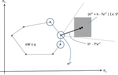
Figure 2.1 A scenario tree with each node representing the outcome of ξt at stage t. . 17 Figure 2.2 A fan-shaped scenario tree. . . 18 Figure 3.1 A 2-dimensional example of the dual problem for Q(xν∗, ξ) with ξ ∈Sk.
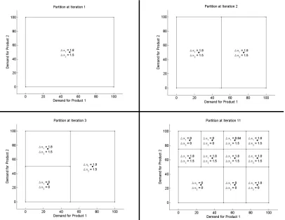
From the possible dual cost vectors, we see that only the circled basic feasible solutions need to be considered when determining bounds for π1 and π2. . . 58 Figure 3.2 A 2-dimensional example of the partition of the random variable support
set at iterations 1, 2, 3, and 11 of the LP-relaxation version of the se-quential bounding algorithm. Conditional mean values for each cell are labelled with a black dot. The quantities ∆π1and ∆π2 are the differences in the bounds on the first two dual decision variables when the random variables are restricted to each cell. . . 69 Figure 3.3 Upper and lower bounds on the optimal objective function value vs.
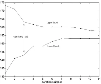
it-eration number for the LP-relaxation version of the sequential bounding algorithm for a two product instance of the inventory problem with down-ward substitutions. The difference between the bounds is the optimality gap. . . 70 Figure 3.4 Experimental results for the modified inventory planning problem,
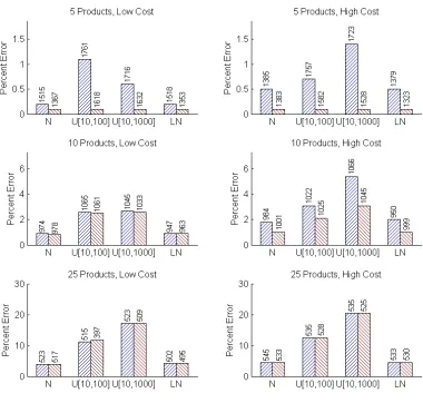
re-ported as percent error. Results are shown for each of 5 sequential bound-ing algorithms, 4 demand distributions, 3 numbers of products, and 2 cost structures. The number of iterations are shown above each bar. . . 72 Figure 3.5 Experimental results for sequential bounding with optimized outcomes
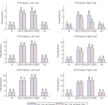
for the modified inventory planning problem, reported as percent error. Results are shown for each of 2 sequential bounding algorithms with op-timized outcomes, 4 demand distributions, 3 numbers of products, and 2 cost structures. The number of iterations are shown above each bar. . . . 74 Figure 3.6 Experimental results for sequential bounding, reported as percent error.
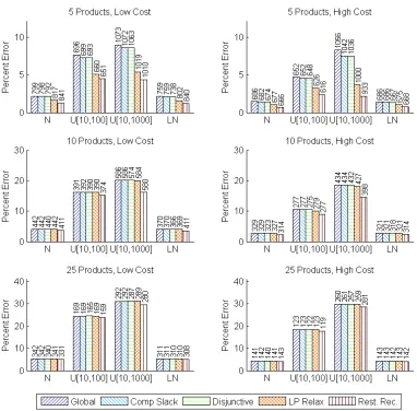
Results are shown for each of 5 sequential bounding algorithms, 4 demand distributions, 3 numbers of products, and 2 cost structures. The number of iterations are shown above each bar. . . 75 Figure 3.7 Experimental results for sequential bounding with optimized outcomes,
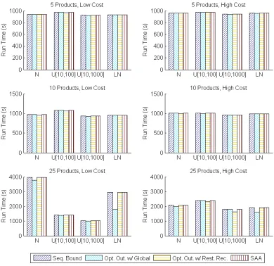
reported as percent error. Results are shown for each of 2 sequential bounding algorithms with optimized outcomes, 4 demand distributions, 3 numbers of products, and 2 cost structures. The number of iterations are shown above each bar. . . 76 Figure 3.8 Run time in seconds for the sequential bounding algorithms, both
Figure 3.9 Experimental results for SAA, reported as estimated percent error. Re-sults are shown for 20 and 100 scenarios for the lower bounding problem, 4 demand distributions, 3 numbers of products, and 2 cost structures. The number of iterations are shown above each bar. . . 79 Figure 3.10 Deterministic bounds for the optimal objective function value. Results
are shown for the optimized outcomes approach with restricted recourse and SAA with 100 scenarios for the lower bounding problem. The test instances include 4 different demand distributions, 3 numbers of products, and 2 cost structures. . . 83 Figure 3.11 Estimate and 99 % confidence bounds for the optimal objective function
value at the final iteration. The estimated objective value is marked with an “x”. Results are shown for the optimized outcomes approach with restricted recourse and SAA with 100 scenarios for the lower bounding problem. The test instances include 4 different demand distributions, 3 numbers of products, and 2 cost structures. . . 84 Figure 4.1 A scenario tree with 6 scenarios . . . 90 Figure 4.2 The effect of splitting the white node on the scenario tree and
correspond-ing support set partition. Black dots in the support set represent mean values over the respective cells. . . 104 Figure 4.3 Flow chart for the rolling horizon simulation approach used to evaluate
effectivness of the algorithms . . . 114 Figure 4.4 Average net profit from the rolling horizon simulation for each of the four
algorithms. Results are shown for a total of 24 test cases, with 3 demand distributions, 2 cost structures, 2 capacity levels, and 2 planning horizon durations. A line connecting the average net profit between two different algorithms indicates that the difference is statistically significant at the 95% confidence level. . . 122 Figure 5.1 A piecewise linear clearing function defined by three points (0,0), (α1, β1),
and (α2, β2). . . 130 Figure 5.2 Example illustration of a 7 period planning horizon with a 2 period rolling
Chapter 1
Introduction
1.1
Overview
Stochastic programming is a branch of mathematical programming that deals with problems of decision making under uncertainty. An emphasis on mathematical programming techniques, such as linear, integer, mixed integer, and nonlinear programming sets stochastic programming apart from other methods for decision making under uncertainty. A broad variety of associated models, properties, and solution algorithms can be found in Birge and Louveaux (1997); Kall and Wallace (1994) and Shapiro et al. (2009).
parameter outcomes.
If the random parameter outcomes for a given stage are independent of past decisions, then the MSLP is considered exogenous; otherwise it is referred to as endogenous. In any solution methodology, we must ensure that decisions are made knowing the distribution of random parameters at future stages, but not the outcomes. For example, in a production environment, a decision maker may need to determine the number of items to produce in a week, an integer decision variable, and the production start time, a continuous decision variable, after reviewing the amount of available inventory and considering uncertain future demand.
Most MSLPs utilize a discrete definition of the underlying random parameters, referred to as a scenario tree. Generating this scenario tree is an important aspect of multi-stage stochastic programming. In most practical problems, the number of possible outcomes of all the random parameters is very large or, in the case of continuous random variables, uncountably infinite. Most efficient solution algorithms rely on consideration of a much smaller subset of outcomes, or scenarios. In multi-stage stochastic programming, random parameters are associated with each stage. Since the decisions and outcomes may depend on decisions and outcomes of previous stages, a scenario tree structure is a natural representation of all outcomes under consideration. Deciding which scenarios to include involves balancing the conflicting objectives of a small problem size with accuracy in the model representation.
variables until a desired level of accuracy or some other termination criterion is reached. Such an approach was first suggested by Birge (1985a).
In the following sections, we define the mathematical notation for an MSLP, including the special case of a two-stage stochastic linear program (2SLP). We also give an example of a multi-stage stochastic linear programming problem for production planning. More general nonlinear stochastic programming formulations are covered elsewhere (Birge and Louveaux, 1997). In the next chapter, we review solution algorithms and associated implementation issues with an emphasis on those methodologies that are likely to be most successful in solving large-scale problems in a reasonable amount of computation time.
1.2
Mathematical Formulations
The following is a mathematical description of a two-stage stochastic linear programming prob-lem.
Minimize z=cx+Q(x) Subject To Ax=b
x≥0 (1.1)
Min c1x1+Eξ2[minx2(ω2)c2(ω2)x2(ω2)
+. . .+EξT|ξ2,...,ξT−1[minxT(ω[T])cT(ω[T])xT(ω[T])]. . .]
s.t. W1x1 =h1
T2(ω2)x1+W2(ω2)x2(ω2) =h2(ω2), ..
.
TT(ω[T])xT−1+WT(ω[T])xT(ω[T]) =hT(ω[T])
x1, xt(ω[t])≥0, t= 2, . . . , T. (1.2)
We use Wt to denote an mt×nt matrix, and xt is the tth stage vector of decision variables of length nt. In stage t,ct is a row vector, ht a column vector, and Tt a matrix of conformal dimensions. We use ξt to denote the vector of random variables associated with stage t, the entries of Tt(ω[t]),ht(ω[t]), andWt(ω[t]) for t= 2, . . . , T. For stage 2 and higher, these random matrices and the decision variables,xt(ω[t]), are indexed onω2 ∈Ω2 andωt∈Ωt(ω[t−1]), the set of outcomes at stage 2 and all other stages t= 3, . . . , T respectively. Here we use the notation ω[t] = (ω2, . . . , ωt) to denote the vector of random outcomes prior to and including stage t. Similarly, the support for ξt is Ξt(ω[t−1]) for t = 3, . . . , T. Sometimes it is convenient to refer to the vector of random problem parameters associated with every stage, ξ= (ξ2, . . . , ξT). The realization of any such random vector is called a scenario, and the realization of any vector ξ[t] = (ξ2, . . . , ξt), with 2≤t ≤T, is called a subscenario. The support set for all scenarios is denoted Ξ ={ξ(ω[T])|ω2 ∈Ω2, . . . , ωT ∈ΩT(ω[T−1])}.
vectors of random variables of all the previous stages. This dependence, and any dependence that decision variables have on previous decisions, is otherwise implicit in the formulation. Of course, there is no dependence on the vectors of random variables associated with future stage outcomes or decisions. This requirement is commonly referred to as non-anticipativity in the stochastic programming literature.
Non-anticipativity can be defined more formally as follows. If we let Ω ={ω[T]} be the set of all outcomes in the sample space, then (Ω,F,P) defines the probability space. Here, F is the sigma field generated from ξT, or σ(ξT). If we let Ft be the sigma field generated by ξt, then we see that{Ft}T
t=2 is a filtration, with Fs⊆ Ft when 2≤s≤t≤T. So, outcomes of the random variable ξs are Ft-measurable whenever s≤ t. In other words, elements in Ft consist of subsets of the elements in Ω with the same history up to and including timet. See Ross and Pek¨oz (2007) for an accessible introduction to measure theory and probability.
Equation 1.2 can be expressed more compactly as follows.
Min c1x1+Q1(x1) s.t. W1x1 =h1
x1≥0.
where the recursive relationship between the first stage functions is
Q1(x1) = Eξ2[Q1(x1, ξ2)] Q1(x1, ξ2(ω2)) = min
x2 {c
and thetth stage recourse function is defined recursively as:
Qt(xt) = Eξt+1|ξ2...ξt[Qt(xt, ξt+1)], t= 2, . . . , T−1
Qt(xt, ξt+1(ω[t+1])) = min xt+1{c
t+1(ω[t+1])xt+1+Qt+1(xt+1)|
Tt+1(ω[t+1])xt(ω[t]) +Wt+1(ω[t+1])xt+1 =ht+1(ω[t+1]);xt+1 ≥0}, t= 2, . . . , T −1
Finally, we define the boundary condition at stage T as:
QT(xT) ≡ 0.
The multi-stage formulation can be viewed as a two-stage formulation with the recourse function replaced by a multi-stage stochastic program with one less stage than the original. In the above formulations, there are no integer restrictions on the decision variables, but these can be added easily, generalizing the problem to a multi-stage stochastic integer program.
Min c1x1,0+PT
t=2
PKt
k=1pkct,kxt,k
s.t. W1x1,0=h1
Tt,kxt−1,a(k)+Wt,kxt,k =ht,k, for all k= 1, . . . , Kt and t= 2, . . . , T.
x1,0, xt,k ≥0, for all k= 1, . . . , Kt, and t= 2, . . . , T. (1.3)
1.3
Production Planning Example
As an example of an MSLP, we consider a single-product, fixed lead-time, finite capacity pro-duction planning problem. At each of a finite number of decision epochs t = 1, . . . , T, the decision maker must determine how many jobsXtto release into the production system. These jobs will immediately become work in process inventory (WIP), and for simplicity, we assume that each job will become part of finished goods inventory (FGI) at the next decision epoch, provided a fixed production capacity constraint is not violated.
The first stage decision variables include:
X1≡ The number of jobs to be released initially at the first decision epoch,
I1 ≡The initial FGI,
B1≡The initial unmet demand,
W1≡The initial WIP inventory,
P1≡ Number of finished goods produced between the first and second decision epochs.
The stage tdecision variables include:
Xt≡The number of jobs released by the decision maker at epoch t,
Bt≡ Cumulative unmet demand at epocht,
Wt≡WIP at epocht,
Pt≡Number of finished goods produced between epochstand t+ 1.
We assume the time between successive decision epochs is sufficiently small that the WIP and FGI is roughly constant in the duration, and production can be used to fulfill demand during the same period. In the formulation below, WIP is always zero in any optimal solution. So, the Wt decision variables are not necessary, but we include them to illustrate how they relate to other decision variables in more complicated formulations.
I1, B1, and W1 are assumed to be known prior to the first decision epoch. Other known parameters include:
Ct ≡ The maximum number of FGI that can be produced between epochs tand t+ 1. γ ≡ The per period discount factor for future costs.
Between two consecutive decision epochs,
cw ≡ Fixed per period unit cost of carrying WIP, ch ≡ Fixed per period unit cost of carrying FGI,
cu ≡ Fixed per period unit cost of cumulative unmet demand, and cp ≡ Fixed production cost per unit.
In addition to these deterministic parameters, there is a stochastic parameter.
Dt(ωt) ≡ The demand for finished goods between epochs t−1 and t.
Min chI1+cuB1+cwW1+cpP1+Q1(X1, I1, B1, W1, P1)
s.t. P1 ≤C1
P1 ≤W1+X1
X1, P1 ≥0
where
Q1(X1, I1, B1, W1, P1) = Eξ2[Q1(X1, I1, B1, W1, P1, ξ2)],
and
Q1(X1, I1, B1, W1, P1, ξ2(ω2)) =
Min γchI2+γcuB2+γcwW2+γcpP2 +Q2(X2, I2, B2, W2, P2)
s.t. W2=W1+X1−P1
I2−B2 =I1−B1+P1−D2(ω2)
P2≤W2+X2
P2≤C2
X2, I2, B2, W2, P2 ≥0.
The recourse function at staget can be written as:
Qt(Xt, It, Bt, Wt, Pt) = Eξt+1|ξ2...ξt[Qt(Xt, It, Bt, Wt, Pt, ξt+1)]
where
Qt(Xt, It, Bt, Wt, Pt, ξt+1(ωt+1)) =
Min γtchIt+1+γtcuBt+1+γtcwWt+1+γtcpPt+1+
Qt+1(Xt+1, It+1, Bt+1, Wt+1, Pt+1) s.t. Wt+1 =Wt+Xt−Pt
It+1−Bt+1 =It−Bt+Pt−Dt+1(ωt+1)
Pt+1 ≤Wt+1+Xt+1
Pt+1 ≤Ct+1
Xt+1, It+1, Bt+1, Wt+1, Pt+1 ≥0. fort= 2, . . . , T −1.
The recourse function for stage T is:
QT(XT, IT, BT, WT, PT) ≡ 0.
2009). This suggests that MSLPs may be more difficult to solve than similarly sized two-stage problems. MSLPs that include integer decision variables are also difficult to solve, since the recourse functions are not guaranteed to be convex. Even if all the random problem parameters are discrete, a relatively modest number of independent random variables results in a very large number of joint outcomes. Assuming independent variables at each stage, the total number of possible outcomes is obtained by multiplying the number of outcomes at each stage, causing the resulting scenario tree to grow exponentially in the number of stages. If any of the random parameters are continuous, then there is effectively an infinite number of possible outcomes. In practice, some representative sample of the possible outcomes must be obtained to make the problem tractable.
1.4
Organization of this Document
In this dissertation we present new sequential bounding approaches for two-stage stochastic programs and apply these approaches to a single-period production planning problem with downward product substitutions. We also present a multi-stage sequential bounding approach, and compare this with several other scenario generation approaches for a production planning problem with uncertain demand and constant work in process inventory. Finally, we consider a multi-stage stochastic program to model the evolution of demand forecasting for production planning with load dependent lead times. We compare a sequential bounding approach to solving this model with other solution methodologies.
In Chapter 3 we study sequential bounding for two-stage stochastic programs. We extend the approach developed by Denton and Gupta (2003) to more general two-stage stochastic problems. The structure of these problems is studied and methods for improving convergence are explored. In particular, we develop methods for tightening bounds on dual and primal decision variables and optimally selecting representative outcomes for each scenario. The sequential bounding approaches are compared to an existing Monte Carlo sampling-based approach for a single-period production planning problem with downward product substitutions.
In Chapter 4 we compare several approaches for scenario tree generation for multi-stage stochastic programming. These include a simple random sampling based approach and two pre-viously published approaches using moment matching and expected value of perfect information (EVPI) to generate the scenario tree. We also propose and evaluate a new sequential bounding approach using dual information. We use a simulation model to evaluate the quality of the solutions for a supply chain management problem in which product demand is continuously distributed at each stage. We use a series of test instances to compare the scenario generation methods on the basis of solution quality, computation time, and difficulty in implementation.
In Chapter 5 we present a multi-stage stochastic program to model the evolution of demand forecasting for production planning subject to load dependent lead times. We use the sequential bounding approach developed in Chapter 4 to solve the MSLP. We compare experimental results with alternative models and solution approaches.
Chapter 2
Literature Review
2.1
Overview
2.2
MSLP Methodologies
2.2.1 Deterministic Equivalent Linear Programs
As shown in Equation 1.3, when the support set of the random problem parameters is finite, we can formulate any multi-stage stochastic programming problem using a deterministic equivalent linear programming problem. This formulation is achieved by indexing decision variables asso-ciated with the second stage and later stages on the set of subscenarios, or the set of all possible past outcomes. Thus, the number of variables and constraints is multiplied by the number of possible outcomes. This can often result in problems that are too large to solve using standard linear programming algorithms, such as the simplex algorithm (Dantzig, 1963) or interior point methods. However, improvements can be made to standard interior point methods for solving two-stage deterministic equivalent linear programming problems (Birge and Holmes, 1992).
2.2.2 L-shaped Method and Nested Decomposition
In the special case of two stages, continuous decision variables, and discrete random variables, an efficient Benders decomposition approach, the L-shaped method (Van Slyke and Wets, 1969) has been developed based on an outer linearization of the recourse function. A relaxation of the problem is utilized, known as the master problem. This relaxation does not include any of the constraints associated with the second stage decision variables. The master problem is repeatedly modified and solved, progressively refining the outer linear approximation to the recourse function. The master problem solution is passed to subproblems corresponding to the recourse problem for each scenario. The solutions to the scenario subproblems, in turn, provide more information about the recourse function, which is passed to the master problem in the form of valid inequalities, known as feasibility and optimality cuts. The integer L-shaped method adds these valid inequalities within a branch and cut procedure in order to deal with binary integer decision variables (Laporte and Louveaux, 1993).
Similar to the L-shaped method, a master problem consisting of only those constraints and costs associated with the first stage of the problem is defined. However, here the subproblems are MSLPs. We can therefore use Benders decomposition for each subproblem, generating new nested subproblems. The solution process involves passing feasible solutions for a subproblem at one stage to its successor subproblems at the next stage. Those successor subproblems are solved to provide valid inequalities (optimality and feasibility cuts) for the parent problem. Degenerate subproblems are common when using nested decomposition, and in order to reduce runtime associated with degenerate solutions, a partitioning strategy was developed (Birge, 1985a). Within the nested decomposition framework, there are several implementation decisions that must be made, including how much information is passed between the master problem and subproblems before moving to a different stage. The fast forward and fast backward approach was developed and found to be among the most successful of such approaches (Wittrock, 1983; Gassmann, 1990).
2.2.3 Progessive Hedging
2.2.4 Endogenous MSLPs
When the outcome of random problem parameters associated with any particular stage of a stochastic programming problem depend on past decisions, the problem is said to be an endogenous stochastic programming problem. The literature on endogenous stochastic pro-gramming problems is limited (Gupta and Grossmann, 2010; Jonsbraten and Woodruff, 1998). If all endogenous random parameters depend linearly on past decisions, we can reformulate the problem as an exogenous MSLP. For example, consider the endogenous random variable ξ3 =M1x1+M2x2+, where is an independent random variable, xt is a vector of decision variables, and Mt is a fixed matrix associated with stage t. We can define y2 = M1x1 and
y3 =y2+M2x2+to be vectors of decision variables at stage 2 and 3 respectively, replacing
ξ3 withy3 everywhere in the formulation. In order to obtain an exogenous formulation, we can assume random parameters are linearly dependent on past decisions.
Throughout this thesis, we assume that either the underlying stochastic process for MSLP is exogenous, or a suitable exogenous approximation to an underlying endogenous process is possible.
2.3
Scenario Generation Methods
It is often impossible or impractical to solve problems with large or infinite support sets Ξ directly using the methods described in the last section. In such situations, we need some way to approximate the MSLP by another MSLP with a support set that is finite and relatively small. The process of generating this representative finite support set for the random problem parameters of a larger MSLP is called scenario tree generation. In this section, we describe several methods for generating and evaluating the quality of scenario trees.
We begin by defining a scenario tree. For exogenous MSLPs, the realization of random problem parameters may depend on past random variable outcomes, but they are always inde-pendent of past decisions. This fact allows us to model the stochastic process {ξt}T
Stage 1
Stage 2
Stage 3
Stage 4
ξ
2(
ω
12
)
ξ
2(
ω
22)
ξ
2(
ω
32)
ξ
3(
ω
1[3])
ξ
3(
ω
2[3])
ξ
3(
ω
3[3])
ξ
3(
ω
4[3])
ξ
3(
ω
5[3])
ξ
3(
ω
6[3])
ξ
4(
ω
1[4])
ξ
4(
ω
2[4])
ξ
4(
ω
3[4])
ξ
4(
ω
4[4])
ξ
4(
ω
5[4])
ξ
4(
ω
6[4])
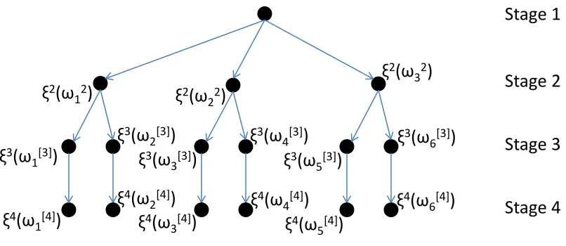
Figure 2.1: A scenario tree with each node representing the outcome of ξt at stage t.
tree data structure as follows. Every level of the tree corresponds to a stage in the MSLP, with the root node corresponding to the first stage and all leaf nodes corresponding to elements of ΞT, the support set for ξT. Every node, except for the root node, has exactly one predecessor node in the previous stage. We use arcs to show this parent-child relationship between nodes in the tree. From this definition, we see that any path from the root node to a node at level t corresponds to a subscenario (ξ2, . . . , ξt). In particular, any path from the root node to a leaf node corresponds to a scenario.
We see that scenario trees are capable of capturing all the dependencies between random problem parameters. An intermediate node at leveltbetween the root and leaf nodes in the tree represents a single outcome of ξt. Since ξt = ξt(ω[t]), may depend on the outcome associated with previous stages, this dependence is captured by the unique sequence of predecessor nodes at earlier stages of the tree.
We provide an example scenario tree in Figure 2.1. This scenario tree has six scenarios, including (ξ2(ω2
2), ξ3(ω22, ω34), ξ4(ω22, ω34, ω44)) where ω [4]
Stage 1
Stage 2
Stage 3
Stage 4
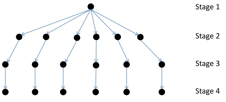
Figure 2.2: A fan-shaped scenario tree.
Next, we consider degeneracy in a scenario tree. Typically most nodes in a scenario tree, other than the root node, will have one or more sibling nodes connected to the same parent node of the previous stage. However, this is not always the case. When a node has only one child node, we will refer to it as degenerate, as in the nodes at stage 4 in Figure 2.1. Here, we see that the four stage stochastic programming problem may be viewed as a three stage problem, where the realization of the random vectorξ4 is known with probability one when the realization of random vector ξ3 is known.
A scenario (ξ2, . . . , ξT) is considered degenerate if every node in that scenario, other than the root node, is degenerate. Similarly, we will say that a stage is degenerate if all the nodes at the corresponding level of the scenario tree are degenerate. An extreme case of degeneracy is the fan-shaped scenario tree of Figure 2.2. In this case, every scenario is considered degenerate because every node other than the root node is associated with only one scenario. Also, every stage is considered degenerate. Here, the four-stage stochastic programming problem can be viewed as a two-stage problem.
in scenario trees. Such a node corresponding to a particular realization of ξt(ω[t]) = ξt(ˆω[t]) is used even in situations where the number of possible realizations of ξt+1((ˆω2, . . . ,ωˆt, ωt+1)) is infinite, or large and finite. Since the number of variables and constraints of an MSLP is often proportional to the number of nodes in the underlying scenario tree, use of such nodes may be necessary to make the resulting MSLP tractable for solution by a computer. However, any model derived from a scenario tree with such nodes will necessarily fail to capture some of the inherent uncertainty associated with decision making.
In many cases, the relative importance of the stages diminishes over time. For example, future returns may be discounted according to an appropriate interest rate if we are trying to maximize total revenue. In these situations, with a limited computational budget, a scenario tree with fewer nodes in later stages may result in a more accurate approximation than one with the same number of nodes at every stage.
Next, we organize the literature on scenario generation into categories. First, we consider non-adaptive methods for generating scenario trees that produce a single scenario tree and often form the starting point for adaptive methods. We also review ideas related to evaluating the quality of scenario trees. These quality measures can also be used in adaptive algorithms, especially if they apply to subtrees of the scenario tree. Finally, we review adaptive methods that involve sequential modifications to a scenario tree in order to improve its accuracy in representing the original MSLP.
2.3.1 Non-adaptive Methods
Sampling Approach
by generating a random sample {ξ2(ωi2)}K1
i=1 of ξ2. We will effectively replace the probability distribution associated withξ2 with the discrete distribution where each member of the sample set is equally likely. Each outcome of this sample set corresponds to a node at the second level of the scenario tree. Next, we generate samples of ξ3 conditioned on the outcomes from the sample for stage 2. The size of these sample sets is simply the number of child nodes for each node corresponding to the outcome of ξ2. We effectively replace the probability distribution of ξ3 conditioned on the outcome of ξ2 with a uniform discrete conditional distribution. The process of conditional sampling continues through each successive stage.
If random problem parameters are independent, then it is not necessary to generate random variables starting with the second stage. In that case, we use a random number generator for each independent random variable. When the distributions associated with random problem parameters depend on other parameters in the same or previous stage, then we must sample from a joint probability distribution function. One method for generating such random numbers is found in Cario and Nelson (1997).
We should point out that sampling described here is sometimes referred to as external sampling (Mak et al., 1999) because it is carried out prior to the solution procedure. This is in contrast to methods that use sampling during the course of the solution algorithm. See Pereira and Pinto (1991) for a description of the Stochastic Dual Dynamic Programming algorithm, which uses sampling to generate an outer approximation of the recourse function at every stage. See Higle and Sen (1991) for a description of the Stochastic Decomposition method for 2-stage stochastic programs, where sampling is used in a cutting plane algorithm. Also, see the related approach of Higle et al. (2010), Stochastic Scenario Decomposition, for multi-stage stochastic programming problems.
ˆ
x∗ with optimal objective function value ˆz∗.
Although we usually cannot directly determine |z∗−zˆ∗|, we can repeatedly generate new and different scenario trees by resampling and resolving the approximating MSLPs. The average objective function value ¯zˆ = N1
s
PNs
i=1zˆ ∗
i for these approximating problems provides a biased estimate of the true optimal objective function value, since E[¯zˆ] ≤ z∗ (Shapiro et al., 2009). Chiralaksanakul and Morton (2004) use the ˆzi∗ values to obtain a lower confidence bound onz∗. With finite second moment and relatively complete recourse assumptions, they also provide an upper confidence bound onz∗through repeated evaluation of feasible policies. When the random parameters between stages are independent, generating such feasible policies involves solving a two-stage stochastic programming problem at every stage. For most situations where random parameters depend on the random parameters of past stages, feasible policies are generated by solving a (T−t+ 1)-stage stochastic program for each staget= 2, . . . , T in the original MSLP. Variance reduction techniques, see Law (2006) for example, are generally useful for reducing the number of scenario trees that need to be generated for a single problem. For example, if the MSLP represents a problem of maximizing revenue subject to random demand at every stage, then antithetic variates might be used to generate a high demand scenario tree whenever a low demand scenario tree is generated. In this way, we hope to reduce the variance associated with ¯
ˆ z.
Importance sampling is among the most important variance reduction techniques for stochas-tic programming because it can be used to improve the accuracy associated with a single scenario tree. Notice that any instance of MSLP can be expressed as the maximization or minimization of a function of the form Rf(x)p(x)dx, where p(x) is a joint probability distribution function for all components of the vector x. Importance sampling involves modifying the function f and replacing p with a different probability distribution function. In other words, we find an appropriate function q such that R
f(x)p(x)dx=R f(x)p(x)
q(x) q(x)dx. Ideally,
f(x)p(x)
sampledf(x) alone. See Dantzig and Glynn (1990) for a description of importance sampling in the context of MSLP.
Importance sampling is especially useful when relatively infrequent events have a high im-pact on the objective function value. We can design q to assign a higher probability to those events. Other heuristic approaches for finding q include finding the best q subject to certain structural assumptions, such as additive separability with respect to the components of x; so, we assume the formq(x) =Pn
i=1qi(xi).
Distribution Approximation Methods
Pennanen and Koivu (2002) uses quadrature rules for sampling to approximate the distribution function. So, if we cast the objective function of MSLP as a multi-variable integration problem
R
f(x)p(x)dx, with p the joint distribution function, and x the vector of all decision variables from all stages, then this approach uses quadrature rules for p. The article points out that the objective function itself, f, is not taken into account in this approach, citing the difficulty in doing so.
Pflug (2001) takes a similar approach to solving MSLP by approximating p with a discrete distribution ˜p. Given that f satisfies a Lipschitz condition, we can find an upper bound on the difference between the optimal objective function value associated with p and the optimal objective function value associated with ˜p. This upper bound can be minimized by selecting the best ˜p that maintains a pre-determined scenario tree structure.
Moment Matching Approach
between the statistical properties of the scenario tree and the underlying random process. These nonlinear programs often must be solved heuristically to determine the probabilities and values associated with the random problem parameters at each node of the scenario tree (Høyland and Wallace, 2001). Miller and Rice (1983) explain how moment matching can be implemented with Gaussian quadrature points. In a pension plan optimization problem, Kouwenberg (2001) found that the performance of a moment matching approach was substantially better than simple external sampling.
In many situations a probability distribution for modeling the random problem parameters is not available. This may be the result of insufficient data or if we fail to find an adequate probability distribution to fit existing data. The moment matching approach is particularly attractive in these cases, since we can limit ourselves to estimating moments and correlation coefficients rather than full joint probability distribution functions.
Optimal Design
Often scenarios that take specific requirements into account, such as the absence of arbitrage opportunities in the context of financial applications, must be enforced in the scenario tree generation process. Some properties of the data in the scenario tree can be enforced, such as adherence to pre-specified moments. In the choice of random problem parameters associated with the scenario tree nodes, as well as the probabilities of their occurrence, we may have considerable freedom in selecting these values.
property. The choice of these statistics is problem specific (Kaut and Wallace, 2007).
Unbiasedness and Stability
In Kaut and Wallace (2007), the importance of unbiasedness and stability are emphasized when evaluating scenario trees. Biasedness is defined as the difference between the optimal objective function values of a sampled problem and the actual problem, or a sufficiently large representation of the actual problem. Stability refers to the difference in objective function values for two optimal solutions associated with two different scenario trees, either with respect to the original problem or with the corresponding sampled problems. Although these criteria can be used in evaluating deteministic methods for scenario tree generation, there must be some mechanism for generating different trees and making comparisons.
2.3.2 Adaptive Methods
Adaptive methods start with a non-adaptive method for scenario tree generation. The scenario tree is assessed according to some measure of quality, which often involves solving an MSLP instance based on the current scenario tree. The scenario tree is then modified in some way in the hope of improving the measure of quality. This process may continue until some termination criterion is reached.
Scenario and Stage Aggregation and Disaggregation
non-homogeneous Markov process can be used to generate conditional outcomes of scenarios, when appropriate.
2.4
Constraint and Variable Aggregation
Stochastic programming problems with continuously distributed random problem parameters can be expressed as infinite dimensional linear programming problems. We can see this in Equation 1.2 from the fact that the constraints are indexed on ωt ∈Ωt for t= 2, . . . , T. Also the decision variables at any stage, except for the first, depend on the outcome of random variables associated with both that stage and past stages. From this perspective, we see that xt(ω[t]) = xt((ω2, . . . , , ωt)) in Equation 1.2 is a function of all past outcomes, and solving the MSLP requires us to find the optimal function for everyt= 2, . . . , T. Even if the support for the random problem parameters is finite, a relatively small number of possible outcomes associated with each stage can result in very large scale deterministic equivalent problems for multi-stage stochastic programs (see Equation 4.2).
In Zipkin (1980b,a), upper and lower bounds for the optimal objective function value of large-scale linear programming problems are found. These bounds are obtained by solving a smaller, but related, linear programming problem based on an aggregation of the constraints and variables of the original problem. Zipkin’s results were established for pure linear pro-gramming problems, with a finite number of constraints and variables, and were made without any reference to stochastic programming. These bounds depend on establishing bounds on the optimal primal and dual decision variables for the original problem.
correspond to the joint conditional probability distribution functions for the outcomes on which the decision variables depend. Wright (1994) develops the results within a measure-theoretic probability framework, allowing for uncertainties in the constraint and cost coefficients.
In the case where random variables are independent and the objective function is a convex function of the random variables, bounds for stochastic programming problems can be found using the classic Edmundson-Madansky and Jensen’s inequalities. The bounds can be made arbitrarily tight by sequentially partitioning the support of the random variables into a succes-sively finer partition and applying the bounds to each new cell of this partition (Huang et al., 1977).
In Denton and Gupta (2003), the L-shaped method with sequential bounding is developed for a two-stage stochastic programming formulation of an appointment scheduling problem. The algorithm iteratively refines a partition of the support set of continuous random parameters associated with the recourse problem. The decision variables found at each iteration converge to an optimal solution, along with the upper and lower bound for the optimal objective function value. The bounds at each iteration are based on those developed by Birge (1985a). From the computational experience with this problem, the authors found that the upper bound converged more slowly to the optimal objective function value than the lower bound.
2.5
Applications
The literature for production planning under uncertainty is also vast. We refer to Mula et al. (2006) for a review of the literature and a classification scheme for the various models that have been developed over the years. They identify 6 research areas where analytical mod-els, like stochastic programming, can be applied: hierarchical production planning, material requirement planning, capacity planning, manufacturing resource planning, inventory manage-ment, and supply chain planning. Of these research areas, perhaps stochastic programming has been applied most often to capacity planning (see Eppen et al., 1989; Morton and Wood, 1999; Huang and Ahmed, 2009). In this dissertation, we focus on manufacturing resource planning and inventory management. In particular, we assume capacity is known, and we determine production and inventory activities prior to the realization of customer demand. We do not consider distributing manufactured goods to multiple locations.
We provide some examples of papers where a real-life problem was used in the development of a stochastic programming problem for production planning. We cover papers where such a model was either developed for, or inspired by, a particular application.
Guan and Philpott (2011) use a multi-stage stochastic quadratic programming problem to model a simplified version of a supply chain planning problem for Fonterra, a New Zealand Dairy company. The authors use the Dynamic Outer Approximation Sampling Algorithm, that they developed, for solving this problem. The authors use simulation to evaluate the optimal policy found using their approach, and they compare this policy with one found by solving a related deterministic model. Although higher expected earnings were achieved with the authors’ model, they feel that a more detailed model would provide a better estimate of the savings.
In Chapter 4, we consider a multi-stage stochastic programming problem developed in the semiconductor industry by Higle and Kempf (2011). The authors consider uncertainty in yields for a multi-stage production process subject to uncertain demand. A constant work in process inventory constraint is used to keep production smooth and inventory holding costs low.
2.6
Contributions of This Dissertation
Chapter 3
Sequential Bounding for Two Stage
Stochastic Linear Programs
3.1
Introduction
For stochastic programs with a very large or an infinite number of scenarios, approximations must be employed. The most common approximation is Monte Carlo sampling, which was first used in the context of sampling-based decomposition by Dantzig and Glynn (1990). Sampling-based methods have been used to estimate statistical confidence intervals on the optimality gap of stochastic programs by Mak et al. (1999) and Glynn and Infanger (2011). The quality of the statistical bounds generated by sampling-based methods depend on the number of scenarios sampled, but larger numbers of scenarios generally result in longer computation times. The number of samples to best trade off computation time and accuracy is problem-specific.
belonging to the corresponding set. Such algorithms can be adapted to a sequential approxi-mation scheme, where the approximate problem is iteratively solved and modified by refining the partition of the support for the random variables until a desired level of accuracy or some other termination criterion is reached. Such an approach was first suggested by Birge (1985a). In this chapter, we describe methods to approximate the solution to two-stage stochastic programs. We present ways to improve the bounds on the approximation error developed by Birge (1985a) in the context of a deterministic sequential approximation algorithm, which we callsequential bounding. In particular, we consider the problem of finding tight bounds on op-timal values of the second stage primal and dual decision variables. Although decision variable bounds are often readily apparent, we show how bounds on the optimal values can be improved for subsets of the random variable support, resulting in faster convergence of sequential bound-ing. We also consider improvements to the restricted recourse bounds of Morton and Wood (1999), which depend on such decision variable bounds. Finally, we consider a mathematical programming approach to find the smallest approximation error by selecting representative outcomes for subsets of the random variable support.
We present three algorithms for bounding the optimal values of primal and dual decision variables. The first algorithm uses linear programming complementary slackness conditions and improves bounds on either the set of primal or dual decision variables by utilizing bounds on the other set of variables. In the absence of primal degeneracy, we show that the tightest upper and lower bound on each primal and dual decision variable is the solution of a corresponding nonlinear program. A linear programming relaxation is utilized in the second algorithm for each of these problems. The third algorithm generates a simplicial cone of dominated dual solutions. This is used to generate a disjunctive linear program for each optimal dual decision variable bound. Finally, we identify special cases where bounds on the optimal decision variables can be found using simple recursion.
sampling-based approach. Computational experiments are based on a collection of test instances for an important stochastic program that arises in the context of semiconductor manufacturing. We compare the deterministic bounds obtained, using sequential bounding with each of the algorithms, to statistical confidence intervals on the optimality gap obtained by Monte Carlo sampling.
The remainder of this chapter is organized as follows. First, we review the relevant literature on bounding methods in Section 3.2. In Section 3.3 the general two-stage stochastic linear programming problem (2SLP) is given, and in Section 3.4 our sequential bounding algorithm is developed for this problem. In Section 3.5 we describe four approaches for finding bounds on the optimal second stage primal and dual decision variables. In Section 3.6 we describe an inventory planning problem with uncertain demand and downward substitutions. We present computational experiments comparing Sample Average Approximation and variations of the sequential bounding algorithm. Conclusions are given in Section 3.7.
3.2
Literature Review
Early work on aggregation bounds was done in the context of deterministic linear programs. In Zipkin (1980b,a), upper and lower bounds for the optimal objective function value of large-scale linear programs were developed. These bounds are obtained by solving a smaller, but related, linear program based on an aggregation of the constraints and variables of the original problem. Aggregate variables and constraints are generated through a linear combination of variables and constraints respectively. The multipliers used in the linear combinations can be viewed as a distribution over rows or columns of the problem parameters in the original linear program. The bounds also depend on establishing bounds on the optimal primal and dual decision variables of the original problem.
conditional joint probability distribution associated with the right hand side values. Similarly, a weighting function is defined for aggregating variables. These weighting functions also cor-respond to the joint conditional probability distribution functions for the outcomes on which the decision variables depend. Wright (1994) extended these bounds within a measure-theoretic probability framework, allowing for uncertainties in the constraint and cost coefficients.
In cases where the objective function is the expected value of a convex function, f, of independent random variables, upper and lower bounds for stochastic programs can be found. The classic Edmundson-Madansky inequality provides an upper bound. This is the expected value of a linear function that overestimatesf. The classic Jensen’s inequality provides a lower bound by evaluating f at the expected value of the random variables. Huang et al. (1977) show these bounds can be made arbitrarily tight by sequentially partitioning the support of the random variables into a successively finer partition and applying the bounds to each new cell of this partition. Many generalizations of these bounds and a variety of other bounding methods have been developed. Morton and Wood (1999) provide an excellent review of these methods.
scheduling problem.
This chapter provides several novel contributions to the existing literature. First, we present several new methods to obtain bounds on optimal values for primal and dual decision variables that can be used to solve two-stage stochastic linear programs in a sequential bounding ap-proach. We identify a class of special problem structures where optimal decision variable bounds can be found using simple recursion. We also develop a new mathematical programming ap-proach to bound the approximation error by replacing random variables with decision variables. Finally, in our computational experiments we directly compare a sampling-based algorithm to sequential bounding, and in some cases, demonstrate that sequential bounding produces the lowest cost solution.
3.3
Two-stage Stochastic Linear Program
The following is a standard formulation for a two-stage stochastic linear program (2SLP):
Min z(x) =cx+Q(x) (3.1)
s.t. Ax=b
x≥0
notation Q(·) to denote the recourse function (see Birge and Louveaux, 1997), which is the expectation over second stage recourse problems. The vector of second stage decision variables of length n2 is denoted y = y(x, ξ) to emphasize its dependence on x and ξ. We use y∗(x, ξ) to denote an optimal solution ofQ(x, ξ). The matrix W(ω) is m2×n2, and the dimensions of the matrix T(ω), the row vector q(ω), and the column vectorh(ω) associated with the second stage have conformal dimensions. Subscripts are used to denote entries of vectors and matrices throughout this chapter. For example, will refer to theithentry ofh(ω) ash
i(ω) and the element in theith row andjth column of T(ω) as Ti,j(ω).
The dual linear programming problem associated with the second stage recourse problem Q(x, ξ(ω)) can be written as follows:
Max π(h(ω)−T(ω)x) (3.2)
s.t. πW(ω)≤q(ω) π unrestricted in sign
We use π =π(x, ξ) for the dual decision variables to emphasize the dependence on x and the random variables ξ, and π∗(x, ξ) is a corresponding optimal solution.
In order to define the dual stochastic program of 2SLP given in Equation 3.1, additional assumptions must be made (see Wright, 1994). First, we restricty(x, ξ(·)) to be in the Lebesgue space, L1(Ω,F, µ;Rn2), for any x ≥0 such that Ax = b. Furthermore, we assume that there
Max vb+Eξ[w(ω)h(ω)] (3.3) s.t. vA+Eξ[w(ω)T(ω)]≤c (3.4) w(ω)W(ω)≤q(ω), a.s. (3.5)
wherevis a row vector of lengthmrepresenting the first stage decision variables, andw(ω) is a row vector of lengthm2 representing the second stage decision variables. Here, the constraints in Equations 3.4 and 3.5 are the first and second stage constraints respectively.
Applying the dual form of the results of Rockafellar and Wets (1976a) to Equation 3.3, an optimal solution, v = v∗ and w = w∗, exists if the following conditions are met: (1) the components of h(ω) are summable, but possibly unbounded, (2) all other components of ξ are bounded, (3) the set of feasible solutions (v, w) is bounded, and (4)wis measurable. For many applications, these conditions are not restrictive, since we can truncate distribution functions for random variables with infinite support with some possible loss of accuracy. Also, most realistic problems do not result in arbitrarily large optimal decision variable values. We will assume that these conditions hold, but alternative conditions to ensure the existence of v∗ and w∗ in Equation 3.3 are provided by Rockafellar and Wets (1976b). Those conditions rely on the existence of feasible solutions satisfying all the constraints with strict inequality. Conditions that do not rely on strict feasibility or a bounded feasible region are provided in Korf (2004).
3.4
Sequential Bounding
Sequential bounding involves partitioning the support set Ξ into disjoint sets Sk such that Ξ = ∪ν
k=1Sk. We also define pk = P{ξ ∈ Sk} and let ˆξk be an arbitrary vector in Sk for
k= 1, . . . , ν. We define the finite support set ˆΞ ={ξˆk}ν
k=1, andP{ξ= ˆξk}=pkfork= 1, . . . , ν. The 2SLP associated with this partitioning of Ξ, which we will refer to as the partitioned value problem (PVP) of 2SLP, can be formulated as follows:
Min zˆν(x,{ξˆk}ν
k=1) =cx+
Pν
k=1pkQ(x,ξˆk) (3.6)
s.t. Ax=b
x≥0
It will be convenient to defineξk =E[ξ|ξ∈Sk] =V ec(hk, Tk, Wk, qk). If we set ˆξk=ξk, we will refer to the resulting PVP as the partitioned mean value problem (PMVP) of 2SLP. The formulation follows:
Min zν(x) =cx+Qν(x) (3.7)
s.t. Ax=b
x≥0
where Qν(x) = Eξ∈Ξˆ[Q(x, ξ)] = Pνk=1pkQ(x, ξk). We denote the optimal objective function value aszν∗, and the optimal solution as (xν∗,{yk,ν∗}ν
k=1). Notice that the PMVP of 2SLP is a standard linear program, and the PMVP of Equation 3.3 is the dual linear program of Equation 3.7. We denote this dual optimal solution as (vν∗,{wk,ν∗}ν
k=1).
is the number of components in ξ. So, for all ω ∈Ω such that ξ(ω) ∈Sk,ai(k) ≤ hi(ω) ≤b(ik), fori= 1, . . . , m2 and am(k2)(j)+i ≤Tij(ω) ≤b(mk)2(j)+i, for i= 1, . . . , m2 and j = 1, . . . , n. Subject to the assumptions of Section 3.3, we note that some of the a and b values can be ±∞; so, Ξ need not be bounded.
Since xν∗ ≥ 0 in the PMVP of 2SLP, we can define bounds L(ik) and Ui(k), for hi(ω)−
Pn
j=1Ti,j(ω)xν ∗
j when ξ(ω)∈Sk, as follows:
L(ik)=a(ik)− n
X
j=1
b(mk) 2(j)+ix
(ν)
j
≤hi(ω)− n
X
j=1
Tij(ω)xνj∗
≤b(ik)− n
X
j=1
a(mk) 2(j)+ix
(ν)
j =U
(k)
i . (3.8)
In Section 3.5 we discuss how these bounds can be used to compute lower and upper bounds on the optimal value of the second stage recourse decisions.
The following result establishes bounds for the recourse function, Q(x), using the PVP. For the special case where the PVP is the PMVP, a more compact version of this proposition and proof is found in Wright (1994), but our proposition and proof allows for equality constraints in the primal problem and non-zeroyk,LBvalues, which lead to tighter bounds onQ(x). Wright (1994) does not allow for arbitrary outcomes associated with each cell of the partition. We use the freedom to select these outcomes to develop tighter bounds on the recourse function in Section 3.4.2. The vectors ˆξk,1,ξˆk,2 ∈ Sk are arbitrary vectors with some of their components fixed to those forξk:
ˆ
ξk,1 =V ec(hk, Tk,Wˆk,1,qˆk,1)
and
ˆ
We defineyk,U B,yk,LB,πk,U B, and πk,LB to be bounds on the second stage recourse decisions:
0≤yk,LB≤y∗(x, ξ)≤yk,U B 0≤πk,LB ≤π∗(x, ξ)≤πk,U B
for all ξ ∈ Sk and k = 1, . . . , ν. Here we use the notation [·]+ = max{·,0}. Also M
i,· denotes theith row andM·,j denotes thejth column of any arbitrary matrix M.
Proposition 1. Supposex is feasible for the first stage constraints of 2SLP,Ax=bandx≥0. Also assume that y∗(x, ξ) and π∗(x, ξ) are bounded for all ξ∈Ξ. Then
ν
X
k=1
pkQ(x,ξˆk,1)−ν1(x,{ξˆk,1}νk=1)≤Q(x)≤ ν
X
k=1
pkQ(x,ξˆk,2) +ν2(x,{ξˆk,2}νk=1),
where
ν1(x,{ξˆk,1}νk=1) = Pν
k=1
Pn2 j=1
h
yjk,U BRSk[π∗(x,ξˆk,1)(W·,j−Wˆ·k,,j1)−(qj−qˆ k,1
j )]+dµ −yk,LBj RSk[−π∗(x,ξˆk,1)(W·,j−Wˆ·k,,j1) + (qj −qˆ
k,1
j )]+dµ
i
ν2(x,{ξˆk,2}ν k=1) =
Pν
k=1
Pm2 i=1π
k,U B i
R
Sk
h
(hi−hˆk,i 2)−(Ti,·−Tˆi,k,·2)x −(Wi,·−Wˆi,k,·2)y∗(x,ξˆk,2)
i+
dµ
−Pν k=1
Pm2 i=1π
k,LB i
R
Sk
h
−(hi−ˆhk,i 2) + (Ti,·−Tˆi,k,·2)x +(Wi,·−Wˆi,k,·2)y∗(x,ξˆk,2)
i+
Proof.
Q(x) = RΞqy∗(x, ξ)dµ
= RΞqy∗(x, ξ)dµ−Pν
k=1
R
Skπ∗(x,ξˆk,1)[W y∗(x, ξ)−h+T x]dµ
≥ R
Ξqy
∗(x, ξ)dµ−Pν
k=1
R
Skπ∗(x,ξˆk,1)[W y∗(x, ξ)−h+T x]dµ
+Pν
k=1
R
Sk[π
∗(x,ξˆk,1) ˆWk,1−qˆk,1]y∗(x, ξ)dµ
= Pν
k=1pkQ(x,ξˆk,1)−
Pν k=1
Pn2 j=1
R
Sk[π
∗(x,ξˆk,1)(W
·,j−Wˆ·k,,j1)−(qj−qˆk,j 1)]y ∗
j(x, ξ)dµ ≥ Pν
k=1pkQ(x,ξˆk,1)−
Pν
k=1
Pn2 j=1
h
yjk,U BR
Sk[π∗(x,ξˆk,1)(W·,j−Wˆ·k,,j1)−(qj−qˆk,j 1)]+dµ −yk,LBj RSk[−π∗(x,ξˆk,1)(W·,j−Wˆ·k,,j1) + (qj−qˆ
k,1
j )]+dµ
i
= Pν
k=1pkQ(x,ξˆk,1)−ν1(x,{ξˆk,1}νk=1)
The second part of the proof is similar to the first.
Q(x) = RΞπ∗(x, ξ)[h−T x]dµ
≤ R
Ξπ
∗(x, ξ)[h−T x]dµ+Pν
k=1
R
Sk(q−π∗(x, ξ)W)y∗(x,ξˆk,2)dµ
= R
Ξπ
∗(x, ξ)[h−T x]dµ+Pν
k=1
R
Sk(q−π∗(x, ξ)W)y∗(x,ξˆk,2)dµ
−Pν
k=1
R
Skπ∗(x, ξ)[ˆhk,2−Tˆk,2x−Wˆk,2y∗(x,ξˆk,2)]dµ
= Pν
k=1pkQ(x,ξˆk,2) +
Pν
k=1
Pm2 i=1
R
Skπ
∗ i(x, ξ)
h
(hi−ˆhk,i 2)−(Ti,·−Tˆi,k,·2)x −(Wi,·−Wˆi,k,·2)y∗(x,ξˆk,2)
i
dµ
≤ Pν
k=1pkQ(x,ξˆk,2) +
Pν
k=1
Pm2 i=1π
k,U B i
R
Sk
h
(hi−ˆhk,i 2)−(Ti,·−Tˆi,k,·2)x −(Wi,·−Wˆi,k,·2)y∗(x,ξˆk,2)
i+
dµ
−Pν
k=1
Pm2 i=1π
k,LB i
R
Sk
h
−(hi−ˆhk,i 2) + (Ti,·−Tˆi,k,·2)x +(Wi,·−Wˆi,k,·2)y∗(x,ξˆk,2)
i+
dµ
= Pν
k=1pkQ(x,ξˆk,2) +2ν(x,{ξˆk,2}νk=1).
The first equality follows from the definition ofπ∗(x, ξ). The next inequality follows fromπ∗(x, ξ) being dual feasible and y∗(x,ξˆk,2) ≥ 0. The next equality follows from the last summation being equal to zero due toy∗(x,ξˆk,2) being feasible. The next equality results from rearranging terms. The last inequality follows from the definition ofπk,LB andπk,U B, establishing the final result.
In general,yk,U B,yk,LB,πk,U B and πk,LB can be difficult to determine efficiently. However, any valid bounds ony∗(x, ξ) andπ∗(x, ξ) will yield valid bounds forQ(x). Ideally we would find sufficiently tight bounds for these second stage decision variables associated with each cell of the partition without too much computational effort. Notice whenQ(x, ξ) has multiple optima, we may select any of the optimal solutions when defining π∗(x, ξ) and y∗(x, ξ). The choice of optimal solutions will in turn determine appropriate values for the decision variable bounds.
Sample Average Approximation (SAA) described by Shapiro and Homem de Mello (1998) and Kleywegt et al. (2002). This establishes bounds on the true objective function value, since:
ˆ
zν(x,{ξˆk,1}νk=1)−ν1(x,{ξˆk,1}νk=1)≤cx+Q(x) =z(x)
and
z(x)≤zˆν(x,{ξˆk,2}νk=1) +ν2(x,{ξˆk,2}νk=1).
The following corollary to Proposition 1 establishes bounds on the optimal objective function value of 2SLP,z(x∗).
Corollary 1. If the assumptions of Proposition 1 hold, then
zν∗−ν ≤z(x∗)≤z(xν∗)≤zν∗+ν2(xν∗,{ξk}νk=1)
where x∗ is an optimal first stage solution of 2SLP and
ν = Pν
k=1
Pn2 j=1y
k,U B j
R
Sk[wk,ν∗(W·,j−W·k,j)−(qj−qkj)]+dµ −Pν
k=1
Pn2 j=1y
k,LB j
R
Sk[−wk,ν∗(W·,j−W·k,j) + (qj−qjk)]+dµ
Proof. The proof of the first inequality follows from z(x∗) = cx∗+Q(x∗) and Proposition 1 with x = x∗, ˆξk,1 = ˆξk,2 = ξk, and π∗(x, ξk) replaced by wk,ν∗. The second inequality follows from x∗ being optimal andxν∗ being feasible in the first stage constraints. The last inequality is a direct consequence of Proposition 1.