Statistical Emulator Construction
for Nonlinear Smart Systems
Francesca D. Reale
1and Ralph C. Smith
2Center for Research in Scientific Computation Department of Mathematics
North Carolina State University Raleigh, NC 27695
Abstract
Comprehensive physical models can accurately quantify the dynamics of nonlinear and hysteretic systems but often require significant computational cost. This can reduce their effectiveness when performing sensitivity analysis, uncertainty analysis, parameter calibration or system design which typically requires multiple iterations of computationally expensive routines. This can also preclude the use of these models for real-time model-based control design. Emulators provide statistical approximations to comprehensive physical models which provide two advantages: high efficiency and statistical characterization of missing model components. We discuss the construction of statistical emulators to provide efficient surrogates for nonlinear smart material models. We will primarily focus on emulators for the homogenized energy model for ferroic compounds.
Keywords: Hysteresis, ferroelectric materials, nonlinear dynamics, statistical emulators
1. Introduction
Smart systems integrate sensors, actuators, and control laws to monitor and respond to external or internal stimuli. Ferroelectric materials are lightweight, low cost, and often can produce broadband responses. Their ease of use and functionality make ferroelectric materials ideal components of a number of smart systems [3]. For example, polyvinylidene fluoride (PVDF) is valuable in acoustic applications such as microphones [6]. High set point accuracy encourages the use of ferroelectric materials in nanopositioning as well. These materials are currently used as capacitors, transducers, and sensors. For example, barium titanate and lead titanate are relatively simple ferroelectric materials that are useful respectively in capacitors and transducers. However, in many applications these materials are increasingly being replaced by lead zirconate titanate (PZT) and lead magnesium niobate (PMN) [3]. For this reason, we focus on models that can characterize the behavior of PMN and PZT.
As a ferroelectric material cools below the Curie point (the phase transition temperature), it incurs a domain structure and spontaneous polarization that can be changed by an applied electric field and/or applied mechanical stress. The domain structure results from the alignment of dipoles that is energetically favorable (minimizes electrostatic and elastic energy) [3]. To use ferroelectric materials in the previously mentioned applications, one must characterize the response to applied field inputs. This includes the field-polarization (E-P) relationship.
In general, the relationship between the input field, stress and the output polarization, strain is nonlinear and hysteretic due to the noncentrosymmetric structure of ferroelectric materials. In low to moderate field levels, one can approximate the E-P relation using a linear model. However, in ferroelectric materials at high field levels, the nonlinear and hysteretic nature of the E-P relationship must be quantified. Furthermore, we desire a model that incorporates stress and temperature-dependence to characterize the behavior of, for example, PZT and PMN. The homogenized energy model incorporates the nonlinear constitutive relations, the lag effect between the inputs and outputs, and thermal relaxation [3]. The model is able to incorporate material nonhomogeneities via
the assumption that certain parameters are manifestations of underlying densities. We consider the computation cost of determining the polarization. We start with a fairly efficient code and have the goal of increasing its efficiency using an efficient surrogate of the polarization along with statistical quantification of missing model components. Later we can expand upon the technique to improve the efficiency of computationally expensive codes. An emulator provides such a statistical approximation of the polarization. To illustrate the technique, we introduce an example of a fairly simple emulator, the Kalman Filter.
We wish to use the Kalman filter as a simple emulator that can predict results. The Kalman filter is a recursive algorithm
Discrete Process
xk =Axk−1+Buk−1+wk−1 (state)
zk =Hxk+vk (measurements)
Prediction
ˆ
xk,−=Axk−1+Buk−1 (projects state)
vk,−=Avk−1AT +Q (projects covariance) Correction
Kk =vk,−HT(Hvk,−HT +R)−1 (updates Kalman gain) ˆ
xk = ˆxk,−+Kk(zk−Hxˆk,−) (updates state)
vk= (I−KkH)vk,− (updates covariance)
(1)
that is used to estimate the state of a dynamic process governed by a linear stochastic difference equation. Let
wk ∼N(0, Q) represent the process noise. Suppose we have measurementszk of the state. Letvk ∼N(0, R)
represent the measurement noise [2, 5]. These measurements are used to update the state estimate via feedback control in the form of a prediction step and a correction step. During the prediction step, we project the state and covariance ahead to obtain the prior estimate and prior estimate error covariance. During the correction step, the projected state is corrected using the measurementszk to obtain the posterior estimate and posterior estimate
error covariance [4, 5]. The discrepancy between the predicted measurements and the actual measurement is termed the residual. Observe that the updated state depends on the product of the residual and the gain. The Kalman gain is used as a “blending factor” to combine the residual with the projected state such that the posterior error covariance is minimized [2, 5]. This combination leads to an updated, better estimate of the state [1]. Therefore we have an estimate with a prescribed statistical uncertainty associated with it that may be improved with each iteration.
2. Homogenized Energy Model
The homogenized energy model (HEM) incorporates the nonlinear and hysteretic constitutive relations, the lag effect between the input field and output polarization, and thermal relaxation. This model is able to characterize cases of nonhomogeneous materials, dipole switching, variable electric fields, and polycrystalline compounds. The material from this section can be found along with further detail in [3].
We consider the negligible thermal relaxation case first. The Gibbs energy
G(E, P, T) =ψ(P, T)−EP (2)
is the difference between the Helmholtz energy
ψ(P) =
1
2η(P+PR) 2, P
≤ −PI
1
2η(P−PR)
2, P ≥P
I
1
2η(PI−PR)2(
P2
PI −PR),|P|< PI
(3)
and the workEP. HerePRandPI respectively denote the remanence and inflection polarization. The resulting
average polarization kernel
¯
P =1
results from the equilibrium condition ∂G∂P = 0. Here δ = +1 for positively oriented dipoles and δ = −1 for negatively oriented dipoles.
We also consider the possibility of thermal relaxation. The Boltzmann relation
µ(G) =Ce−GV /kT (5)
balances the Gibbs energy and the relative thermal energy kT /V where k is Boltzmann’s constant and V is the reference volume. Consider a uniform lattice composed of N = N++N− cells each with a positive or negative dipole orientation. The fraction of positively oriented dipoles x+ = N+/N and negatively oriented dipolesx−=N−/N sum to unity. The average polarizations associated with positively and negatively oriented dipoles are respectively denoted byhP+iandhP−iand are given by
hP+i=
Z ∞
P0(T)
P µ(G)dP, hP−i=
Z P0(T)
−∞
P µ(G)dP. (6)
The local average polarization is
¯
P =x+hP+i+x−hP−i. (7)
We denote the likelihoods of switching from negatively oriented to positively oriented and vice versa respectively byp−+ andp+−. The evolution of dipole fractions is then given by
˙
x+=−p+−x++p−+(1−x+) (8)
where the fractionx− can be obtained using the equationx−+x+= 1.
For a single crystal, the material properties are assumed to be homogeneous and isotropic which implies that the parameters are spatially invariant. However, this assumption is not valid for polycrystalline compounds which exhibit variable effective fields, anisotropy, and material nonhomogeneities. These nonhomogeneous effects are accounted for by assuming that parameters are manifestations of underlying densities.
We consider the interactive and coercive field parameters. The coercive field valueEC =η(PR−PI) indicates
when a dipole switch occurs. A dipole switch will occur at −EC and +EC. The underlying density associated
with EC is denoted by νC. For physical considerations νC ≥ 0, νC is defined only for positive inputs, and
|νC(x)|≤c1e−a1xfor positive constantsa1 andc1. Additionally, neighboring dipoles interact with the applied field to augment the applied fieldE. We denote this interaction field byEI. The underlying density associated
withEI is νI. For physical considerations, νI ≥0,νI is an even function, and|νI(x)|≤c2e−a2|x|for positive constantsa2 andc2. The densities are scaled such that
Z ∞
0
Z ∞
−∞
ν(EC, EI)dEIdEC=C (9)
whereC is a scaling constant andν(EC, EI) is the joint density.
The polarization model is formulated as the integral
[P(E)](t) =
Z ∞
0
Z ∞
−∞
νC(EC)νI(EI)[ ¯P(E+EI;EC, ξ)](t)dEIdEC (10)
whereξis the initial dipole distribution.
We use numerical integration to approximate the value of the integral. Thus the integral is represented as the sum
[P(E)](t) =
Ni
X
i=1
Nj
X
j=1
νC(ECi)νI(EIj)[ ¯P(E+EIj;ECi, ξj)](t)viwj (11)
where the abscissasEIj, ECi and their respective weights vi,wj are given by the chosen quadrature formula,
To illustrate for the interaction field, the points EIj and weights wj for the four-point truncated
Gauss-Legendre quadrature rule used on each subinterval [hq−1, hq] of [−L, L] are
EIq1 = hq−1+h
1 2−
√
15+2√30 2√35
, wq1 =
49h
12(18+√30)
EIq2 = hq−1+h
1 2−
√
15−2√30 2√35
, wq2 =
49h
12(18−√30)
EIq3 = hq−1+h
1 2+
√
15−2√30 2√35
, wq3 =
49h
12(18−√30)
EIq4 = hq−1+h
1 2+
√
15+2√30 2√35
, wq4 =
49h
12(18+√30)
(12)
wherehq=−L+qhandh= 2L/Nq. The coercive field quadrature points and weights are defined similarly on
Np subintervals. We note that throughout the analysis, we set the number of subintervals for the interactive
field and coercive field densities to be equal so thatNq =Np.
3. Negligible Thermal Relaxation
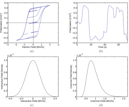
We first examine the outputs of the numerical implementation of the homogenized energy model under the assumption of negligible thermal relaxation. The relationship between the input field and output polarization is presented in Figure 1(a). We provide the polarization over a 73 second interval in Figure 1(b). The number of abscissas is chosen so that both the normal interactive field density and the lognormal coercive field density are sufficiently smooth. The field densities obtained when the number of subintervals Nq = Np = 20 are
shown in Figure 1(c) and Figure 1(d). Note that there are 80 coercive field and 80 interactive field quadrature points. The computation time to obtain the approximation of the polarization (10) from four-point truncated Gauss-Legendre quadrature onNp=Nq = 20 subintervals is approximately 0.16 seconds. All future results are
compared to this baseline approximation of (10). We run the computations to compute the baseline as well as subsequent approximations of the polarization on a Dell Optiplex 755 with an Intel(R) Core(TM)2 Quad CPU @ 2.40GHz with 3 GB of RAM.
Using the Kalman Filter algorithm (1), we blend two approximations of the polarization integral (10) to obtain a better estimate. The goal is to reduce computation time while producing numerical results that accurately replicate the baseline results. We reduce computational time by reducing the number of quadrature points used in the approximation of the integral (10). We begin by reducing the number of intervals to reduce the number of abscissas. The number of quadrature points is reduced further by implementing a lower order Gaussian quadrature rule. Additionally, we consider a Newton-Cotes formula to exploit uniform abscissa spacing as a means of reducing computational time.
3.1 Gaussian Quadrature
We suggest a strategy to reduce computational time. We compute the polarization iteratively over a 73 second interval with time increments of 5×10⁻² seconds. This computation yields 1,461 polarization values. LetPn,mbe the vector of 1,461 polarization values that result from using ann-point truncated Gauss-Legendre
quadrature rule onmintervals to approximate the value of the integral (10). Recall that the results of Figure 1 are obtained by utilizing the 4-point quadrature rule on N = 20 intervals. We use P4,20 as a baseline for comparison against other results. Consider two polarization vectors Pn1,m1 and Pn2,m2. Let σ
2
n,m be the
variance of the difference betweenPn,mandP4,20 divided by the total number of quadrature points associated with calculatingPn,m. There are a total of 2×n×mpoints involved in the calculation ofPn,m. Assume that
Pn2,m2 is a more accurate calculation with respect toP4,20 thanPn1,m1. TakePn1,m1 to be the initial estimate
of the polarization vector with uncertainty σ2
−3 −2 −1 0 1 2 3 −0.4
−0.3 −0.2 −0.1 0 0.1 0.2 0.3 0.4
Electric Field (MV/m)
Polarization (C/m
2 )
0 20 40 60
−0.4 −0.3 −0.2 −0.1 0 0.1 0.2 0.3 0.4
Polarization (C/m
2 )
Time (s)
(a) (b)
−0.4 −0.2 0 0.2 0.4 0
0.2 0.4 0.6 0.8 1 1.2
x 10−6
Interactive Field (MV/m)
Interactive Field Density
0 0.5 1 1.5 2 2.5 0
0.2 0.4 0.6 0.8 1 1.2
x 10−6
Coercive Field (MV/m)
Coercive Field Density
(c) (d)
Figure 1: (a) Field-polarization relationship, (b) the polarization over a 73 second interval, (c) the interactive field densityνI, and (d) the coercive field densityνC.
Pn2,m2 with uncertaintyσn2,m2 < σn1,m1. Based on the Kalman Filter algorithm presented in (1), we propose
that the estimate ˆx(i) of theithpolarization vector componentP(i)
4,20 be given by
ˆ
x(i) = P(i)
n1,m1+K1(P
(i)
n2,m2−P
(i)
n1,m1) (13)
or, equivalently,
ˆ
x(i) = K2Pn(1i),m1+K1P
(i)
n2,m2 (14)
where we compute the gain
Ki=
σ2
ni,mi
σ2
n1,m1+σ
2
n2,m2
(15)
fori= 1, . . . ,1461. We may compute subsequent estimates of the polarization by updating the variance, gain, and polarization prediction as suggested by the Kalman Filter algorithm. This option will not be explored here, but will be considered in the future.
approximation and theP4,4 approximation as separate “measurements.” We compare both approximations to theP4,20approximation to obtain values of the uncertainty of these approximations
σ2
4,2 = 3.4781×10⁻⁵
σ2
4,4 = 7.5186×10⁻⁷
(16)
which are used to compute the gains
K1 = 2.1160×10⁻²
K2 = 9.7884×10⁻¹.
(17)
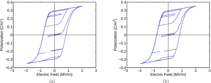
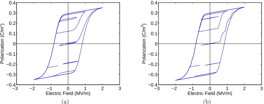
Using these two approximations and their associated uncertainties, we find an estimate for each polarization value. This results in the approximation ˆxG of the polarization vectorP4,20. Figure 2 displays the comparison ofP4,20and the approximation obtained withP4,2andP4,4. Figure 2(a) presents the polarizationP4,20whereas Figure 2(b) displays the approximation ˆxG. The mean absolute difference between these two vectors of 1,461
values is 2.9205×10⁻³. We also compare the time required to obtain both approximations. It takes around 0.16 seconds to obtainP4,20 whereas it takes just over 0.03 seconds to obtain ˆxG. The latter time includes the
0.02 seconds it takes to obtainP4,4and the 0.01 seconds to obtainP4,2 as well as the time required to combine them as suggested in (14).
Figure 2 demonstrates that the approximation ˆxG does not appear as smooth as the P4,20 polarization. While other smoothing techniques are considered, we choose to use moving average due to its simplicity and its efficiency.
The moving average technique averagesma-many data points at a time to smooth out noisy, ordered data.
We test the valuesma = 3,5,7. We choose to averagema = 5 points at a time to smooth the approximation
ˆ
xG and obtain a closer approximation toP4,20. Let ˆxG,S(i) be the ithcomponent of the smoothed ˆxG. Then the
ithcomponent of the approximation ˆx G,S is
ˆ
x(G,Si) = 1 5
4+i
X
n=i
ˆ
x(Gn) (18)
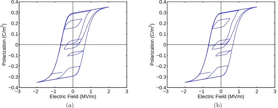
for i = 1, . . . ,1457. It takes just over 10−3 seconds to run. Figure 3 presents the comparison between the baselineP4,20 and the approximation ˆxG,S. The resulting mean absolute difference fromP4,20is 2.4257×10⁻³.
−3 −2 −1 0 1 2 3 −0.4
−0.3 −0.2 −0.1 0 0.1 0.2 0.3 0.4
Electric Field (MV/m)
Polarization (C/m
2 )
−3 −2 −1 0 1 2 3 −0.4
−0.3 −0.2 −0.1 0 0.1 0.2 0.3 0.4
Electric Field (MV/m)
Polarization (C/m
2 )
(a) (b)
−3 −2 −1 0 1 2 3 −0.4
−0.3 −0.2 −0.1 0 0.1 0.2 0.3 0.4
Electric Field (MV/m)
Polarization (C/m
2 )
−3 −2 −1 0 1 2 3 −0.4
−0.3 −0.2 −0.1 0 0.1 0.2 0.3 0.4
Electric Field (MV/m)
Polarization (C/m
2 )
(a) (b)
Figure 3: (a) Relationship between the field and the baseline approximation of the polarizationP4,20and (b) field versus the approximation ˆxG,S.
3.2 Gaussian Quadrature:
n
-point Rules
To reduce the computational time further without a significant increase in the mean absolute difference from
P4,20, we utilize the one-, two-, and three-point truncated Gauss-Legendre quadrature rules. The total number of abscissas used to approximate the integral (10) with n-point truncated Gauss-Legendre quadrature on m
subintervals is 2×n×m. Recall we setNq =Np=m.
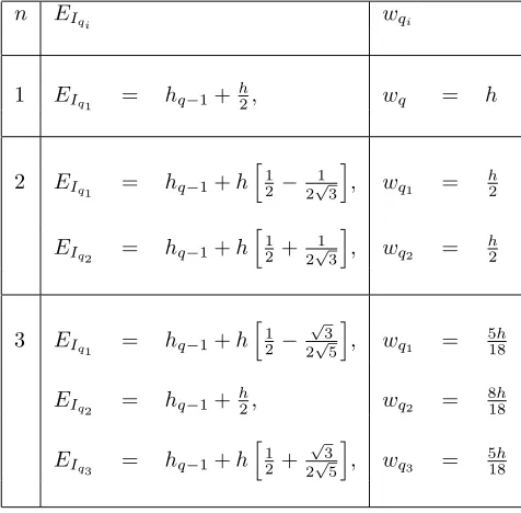
To illustrate for the interaction field, we provide the points EIj and weights wj for the n-point truncated
Gauss-Legendre quadrature rule used on each subinterval [hq−1, hq] of [−L, L] in Table 1 wherehq =−L+qh
andh= 2L/Nq. The coercive field quadrature points and weights are defined similarly on Np subintervals.
TheP1,4approximation and theP3,4approximation are used as separate “measurements.” Both
approxima-n EIqi wqi
1 EIq1 = hq−1+
h
2, wq = h
2 EIq1 = hq−1+h
h
1 2−
1 2√3
i
, wq1 =
h
2
EIq2 = hq−1+h
h
1 2+
1 2√3
i
, wq2 =
h
2
3 EIq1 = hq−1+h
h
1 2−
√ 3 2√5
i
, wq1 =
5h
18
EIq2 = hq−1+
h
2, wq2 =
8h
18
EIq3 = hq−1+h
h
1 2+
√ 3 2√5
i
, wq3 =
5h
18
tions are compared to theP4,20approximation to obtain measures of the uncertainty of these approximations
σ2
1,4 = 4.5902×10⁻⁴
σ2
3,4 = 1.9520×10⁻⁶ (19)
which are used to compute the gains
K1 = 4.2346×10⁻³
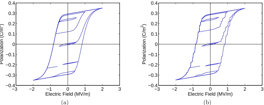
K3 = 9.9577×10⁻¹. (20) We obtain ˆxR by blending the approximations P1,4 and P3,4. We compare the result to the baseline P4,20 to find that the mean absolute difference between the two vectors is 4.6230×10⁻³. It takes about 0.027 seconds to obtain ˆxR compared to 0.16 seconds to compute P4,20. Figure 4 illustrates the comparison of the baseline
P4,20 to the approximation ˆxR.
We apply moving average by averagingma = 5 points at a time to smooth out ˆxR. The smoothing takes
just over one-thousandth of a second and yields a mean absolute difference of 3.9425×10⁻³. Let ˆx
R,S denote
the smoothed ˆxR approximation. Figure 5 presents the comparison of the baselineP4,20 to the approximation ˆ
xR,S.
−3 −2 −1 0 1 2 3 −0.4
−0.3 −0.2 −0.1 0 0.1 0.2 0.3 0.4
Electric Field (MV/m)
Polarization (C/m
2 )
−3 −2 −1 0 1 2 3 −0.4
−0.3 −0.2 −0.1 0 0.1 0.2 0.3 0.4
Electric Field (MV/m)
Polarization (C/m
2 )
(a) (b)
Figure 4: (a) Hysteretic relationship between the field and the baseline approximation of the polarizationP4,20 and (b) field versus the polarization estimate ˆxR.
3.3 Trapezoid Rule
The approximations in Subsections 3.1 and 3.2 utilize Gaussian quadrature rules. Now the uniform abscissa spacing of Newton-Cotes quadrature rules is exploited to further reduce computational time. We illustrate the trapezoid rule for the interactive field. Consider a trapezoid rule approximation of the integral over [−L, L]. LetNt be the number of quadrature points. The Newton-Cotes rules use uniformly spaced quadrature points
xk =−L+khwhereh=N2tL−1 is the stepsize andk= 0,1, . . . , Nt−1. Letyk be the value of the integrand at
xk. Then the integral is approximated byh(12y0+y1+. . .+yNt−2+
1
2yNt−1). The trapezoid rule for the coercive
field is defined similarly. Observe that a benefit of using uniformly spaced quadrature points is that one can reuse some abscissas as one increases the number of abscissas. So one may reuse previous calculations resulting in less computational cost. Let us callPNt the vector of 1,461 polarization values obtained when the trapezoid
rule with Nt abscissas is used. We avoid calculation of the logarithm of zero by setting any zero quadrature
point to machine epsilon 2.2×10⁻¹⁶.
−3 −2 −1 0 1 2 3 −0.4
−0.3 −0.2 −0.1 0 0.1 0.2 0.3 0.4
Electric Field (MV/m)
Polarization (C/m
2 )
−3 −2 −1 0 1 2 3 −0.4
−0.3 −0.2 −0.1 0 0.1 0.2 0.3 0.4
Electric Field (MV/m)
Polarization (C/m
2 )
(a) (b)
Figure 5: (a) Relationship between the field and the baseline approximation of the polarizationP4,20and (b) field versus the approximation ˆxR,S.
prediction strategy. As noted earlier, the components of the vectorP4,20are assumed to be the true polarization values.
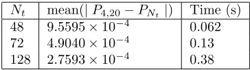
We wish to find the number of trapezoid rule points necessary to compute polarization values comparable to the P4,20 values. We test numerous values of Nt. We visually and numerically compare PNt to P4,20 for
varying values ofNt. The mean absolute difference from theP4,20vector of polarization values is on the order of 10−4 for each vector. The results are displayed in Table 2 and in Figure 6. Note the time required to obtain the polarization vector P4,20 is about 0.16 seconds. We note that the polarization computed whenNt = 72
abscissas are used appears sufficiently accurate.
Similar to what is presented in (14), we propose that theithprediction ˆx(i)of the polarization be given by
ˆ
x(i)=K2PN(it1) +K1P
(i)
Nt2 (21)
where we compute the gain
Ki=
σ2
Nti
σ2
Nt1 +σ
2
Nt2
(22)
fori= 1,2, . . . ,1461.
We use theP4 approximation and theP9 approximation as separate “measurements.” It takes about 0.024 seconds to blend the two approximations to obtain the Kalman approximation ˆxT. We compare the result to
theP4,20 approximation and find a mean absolute difference of 8.7363×10⁻³. We smooth this approximation to obtain the estimate ˆxT,S. The smoothing step takes one-thousandth of a second. The mean absolute
difference between the approximation ˆxT,S and the baselineP4,20 is 7.6445×10⁻³. The visual comparison to the approximationP4,20presented in Figure 7.
Nt mean(|P4,20−PNt |) Time (s)
48 9.5595×10⁻⁴ 0.062 72 4.9040×10⁻⁴ 0.13 128 2.7593×10⁻⁴ 0.38
Table 2: Numerical and chronological comparison of trapezoid rule approximationPNt of (10) to the baseline
0 20 40 60 −0.4
−0.3 −0.2 −0.1 0 0.1 0.2 0.3 0.4
Time (s)
Polarization (C/m
2 )
P
4,20
Pt
48
Pt
72
Pt
128
39 40 41 42 −0.2
−0.195 −0.19 −0.185 −0.18
Time (s)
Polarization (C/m
2 )
P
4,20
Pt
48
Pt
72
Pt
128
(a) (b)
Figure 6: (a) Comparison of the trapezoid rule approximationsPNt to the baseline approximationP4,20 over a
73 second interval and (b) expanded view of the approximations.
−3 −2 −1 0 1 2 3 −0.4
−0.3 −0.2 −0.1 0 0.1 0.2 0.3 0.4
Electric Field (MV/m)
Polarization (C/m
2 )
−3 −2 −1 0 1 2 3 −0.4
−0.3 −0.2 −0.1 0 0.1 0.2 0.3 0.4
Electric Field (MV/m)
Polarization (C/m
2 )
(a) (b)
Figure 7: (a) Relationship between the field and the baseline approximation of the polarizationP4,20and (b) field versus the approximation ˆxT,S.
3.4 Summary of Negligible Thermal Relaxation Results
A summary of the results from Section 3 is presented in Table 3. We observe that the computational cost of all three Kalman Filter estimates is the same to one significant figure. The approximation ˆxG,S corresponds
to the least mean absolute difference from the baseline approximationP4,20. Thus the preferred strategy is to obtain two four-point Gaussian quadrature rule approximations onm≤20 intervals and blend them using the Kalman Filter algorithm as proposed in (14).
4. Thermal Relaxation
The homogenized energy model is able to incorporate thermal relaxation. Section 3 covers the details of the negligible thermal relaxation case. When thermal relaxation is incorporated, the calculations are significantly slower.
LetRn,mbe the vector of 1,461 polarization values that result from using ann-point quadrature onm
Approximation ˆx mean(|P4,20−xˆ|) Time (s)
P4,20 0 0.16
ˆ
xG,S 2.4257×10⁻³ 0.031
ˆ
xR,S 3.9425×10⁻³ 0.028
ˆ
xT,S 7.6445×10⁻³ 0.025
Table 3: Numerical and chronological comparison of approximations to the baseline approximationP4,20.
R4,20 is presented in Figure 8(a). We use R4,20 as a baseline for comparison against other approximations of the polarization.
We blend the two measurementsR4,2 and R4,4 using the Kalman filter strategy suggested by (14). This yields the vector of polarization values ˆxT R. It takes about 1.14 seconds to obtain the baselineR4,20. We blend
R4,2 andR4,4 to obtain the smoothed approximation ˆxT R in 0.13 seconds. The mean absolute difference from
R4,20 is 1.8190×10⁻³. Figure 8(b) displays the field versus the smoothed polarization ˆxT R.
−3 −2 −1 0 1 2 3 −0.4
−0.3 −0.2 −0.1 0 0.1 0.2 0.3 0.4
Electric Field (MV/m)
Polarization (C/m
2 )
−3 −2 −1 0 1 2 3 −0.4
−0.3 −0.2 −0.1 0 0.1 0.2 0.3 0.4
Electric Field (MV/m)
Polarization (C/m
2 )
(a) (b)
Figure 8: (a) Relationship between the field and the baseline approximation of the polarizationR4,20 and (b) the field versus the approximation ˆxT R smoothed with moving average.
5. Concluding remarks
The results of this investigation demonstrate that the Kalman filter works well as an emulator for approxi-mating polarization in the homogenized energy model. We achieve a greater than 80% reduction in computation time while consistently maintaining a mean absolute difference from baseline of less than 10−2. This was accom-plished using one iteration of the Kalman Filter strategy. Consideration of multiple iterations of the Kalman Filter strategy should be beneficial in reducing the mean absolute error at the cost of a minor time increase for subsequent iterations and updated estimates of the state, variance, and gain. Other emulators may provide additional benefits and will be considered in future work.
Acknowledgments
References
[1] Gershenfeld, N.,The Nature of Mathematical Modeling, Cambridge, Cambridge, 1999.
[2] Grewal, M.S. and Andrew, A.P.,Kalman Filtering: Theory and Practice Using MATLAB, John Wiley and Sons, Hoboken, NJ, 2008.
[3] Smith, R.C.,Smart Material Systems: Model Development, SIAM, Philadelphia, 2005.
[4] Stengel, R. F.,Optimal Control and Estimation, Dover, New York, 1994.
[5] Welch, G. and Bishop,G.,An Introduction to the Kalman Filter, University of North Carolina, Department of Computer Science, TR 95-041, July 24, 2006<http://www.cs.unc.edu/ welch/kalman/kalmanIntro.html>.