Sharp-Fin Induced Shock Wave/Turbulent Boundary Layer Interactions over a Cylindrical Surface.

(1)

ABSTRACT

PICKLES, JOSHUA DAVID. Sharp-Fin Induced Shock Wave/Turbulent Boundary Layer Interactions over a Cylindrical Surface. (Under the direction of Venkateswaran Narayana-swamy and Pramod Subbareddy.)

Interactions between an oblique shock wave generated by a sharp fin placed on a

cylindrical surface and the incoming boundary layer are investigated to unravel the mean

features of the resulting shock/boundary layer interaction (SBLI) unit. It is the goal of this

dissertation to establish the mean response of a fin-on-cylinder SBLI in both unperturbed

and perturbed incoming boundary layer conditions, and to investigate whether the

non-linear actions between a shock wave and perturbed incoming boundary layer can be used

to engender control forces required for improved maneuverability and vehicle performance.

This fin-on-cylinder SBLI unit has several unique features caused by the 3-D relief offered

by the cylindrical surface that noticeably alter the shock structure.

Complementary experimental and computational studies are made to delineate both

the surface and off-body flow features of the fin-on-cylinder SBLI unit and to obtain a

detailed understanding of the mechanisms that dictate the mean flow and wall pressure

features of the SBLI unit. Results show that the fin-on-cylinder SBLI exhibits substantial

deviation from quasi-conical symmetry that is observed in planar fin SBLI. Furthermore,

the separated flow growth rate appears to decrease with downstream distance and the

separation size is consistently smaller than the planar fin SBLI with the same inflow and

fin configurations. The causes for the observed diminution of the separated flow and its

downstream growth rate were investigated in the light of changes caused by the cylinder

curvature on the inviscid as well as separation shock. It was found that the inviscid shock

gets progressively weakened in the region close to the triple point with downstream distance

due to the 3D relief effect from cylinder curvature. This weakening of the inviscid shock

feeds into the separation shock, which is also independently impacted by the 3D relief, to

(2)

Having established the baseline (unperturbed) flow response, well-quantified

distor-tions are generated via micro-ramp vortex generators (VG) to embed strong streamwise

vortices into the boundary layer. These VGs are 1.0 and 0.6 incoming boundary layer

thick-nesses tall, and their geometries are configured for maximum distortion strength. The

analog control forces and moments are determined using the mean surface pressure field

for different VGs placed at different azimuthal locations with respect to the fin leading edge.

These configurations resulted in up to 23%, 22% and 5% change in the fin-normal force,

rolling and pitching moments, respectively, compared to the unperturbed results. The

im-pact on the control moments provides compelling evidence that perturbing the boundary

layer and exploiting the associated fin-generated shock boundary layer interactions is a

viable strategy to enable high maneuverability in munitions via dramatic changes in the

(3)

(4)

Sharp-Fin Induced Shock Wave/Turbulent Boundary Layer Interactions over a Cylindrical Surface

by

Joshua David Pickles

A dissertation submitted to the Graduate Faculty of North Carolina State University

in partial fulfillment of the requirements for the Degree of

Doctor of Philosophy

Aerospace Engineering

Raleigh, North Carolina

2019

APPROVED BY:

Jack Edwards Kenneth Granlund

Venkateswaran Narayanaswamy Co-chair of Advisory Committee

(5)

DEDICATION

(6)

BIOGRAPHY

Joshua Pickles, born and raised in Raleigh, North Carolina, attended North Carolina State

University for his undergraduate and graduate academic careers. He obtained is Bachelor’s

Degree in Aerospace Engineering in 2015, and immediately continued into graduate school

under the co-advisement of Drs. Venkat Narayanaswamy and Pramod Subbareddy. While

working as a research assistant under Dr. Narayanaswamy on investigating the effect of

3-D relief on sharp-fin induced shock wave/boundary layer interactions, Joshua received is

Master’s Degree in 2019 in Aerospace Engineering and continued on the same program to

(7)

ACKNOWLEDGEMENTS

To my advisor, Dr. Venkat Narayanaswamy, thank you for the opportunity and guidance

that has allowed me to develop the skillset of a professional engineer and researcher in

fluid dynamics. Further, I wish to thank my Ph.D. committee Drs. Pramod Subbareddy, Jack

Edwards, and Kenneth Granlund for their direction and assistance in my research and their

classes. Thank you to the other graduate faculty and specialty trade technicians, without

whom this work would not have been possible. To my friends and colleagues who I have had

the pleasure to meet over the years: Thank you for your support and the laughs, especially

during the late nights in the lab. This process would have been much less enjoyable without

you. I specifically wish to thank my colleague Bala Mettu, and Ben Kirschmeier and his

advisor Dr. Matthew Bryant for their assistance in performing the CFD presented in this

work and in 3-D printing the vortex generators, respectively. To my parents and my brother,

who never stopped believing in me and provided me with support when I needed it the

most. Thank you for the opportunity and instilling in me the desire and work ethic to

push myself. Finally, I wish to thank Dr. Matthew Munson and the Army Research Office

for providing the financial support under grant W911NF-16-1-0072 that made this work

(8)

LIST OF TABLES

Table 2.1 Incoming flow and boundary layer characteristics . . . 21

Table 4.1 Freestream values and characteristics of the incoming boundary layer. 65

Table 5.1 Incoming flow and boundary layer characteristics . . . 86 Table 5.2 Comparison of the theoretical predictions of the plateau wall

pres-sure between S1 and S2 with experimental values at different stream-wise locations of fin-on-cylinder SBLI. . . 114

(12)

LIST OF FIGURES

Figure 1.1 Sketch ofλ-shock structure: (a) streamwise and (b) top views, based on[Alv92]. . . 7 Figure 1.2 Illustration of fundamental modifications to the inviscid shock

struc-ture generated in a fin-on-cylinder configuration. . . 14

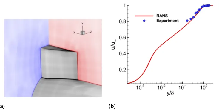
Figure 2.1 Representation of the (a) fin-on-cylinder and (b) planar fin models used in the experimental investigations. . . 20 Figure 2.2 PLS schematic. . . 25 Figure 2.3 (a) Illustration of the grid generated for the Euler and RANS

simu-lations used in this study. (b) Boundary layer profile comparison between the RANS and the experiment. . . 28

Figure 3.1 Schematic of the fin-on-cylinder configuration. . . 37 Figure 3.2 Schematic of the SBLI configuration and the PLS setup used for the

experiments. . . 39 Figure 3.3 a) Overlay of the grid cross-section with the line contour plot for

density at 20 mm (x/R=0.8) from the fin leading edge. b) Boundary layer profile comparison between the RANS and the experiment. . . 40 Figure 3.4 PLS calibration Schematic. . . 41 Figure 3.5 PLS calibration data obtained in the present study along with a cubic

polynomial fit and the comparison of the corresponding computed values of silicone oil droplets using the de-agglomeration data of [Bra87]. . . 42 Figure 3.6 A representative instantaneous PLS field after background

subtrac-tion and laser sheet correcsubtrac-tion obtained at x/R=1.0. The flow direc-tion is into the page. . . 46 Figure 3.7 Ensemble averaged freestream normalized PLS images at different

streamwise locations: a) x/R=0.4, b) x/R=0.8 and c) x/R=1.0. Flow is into the page. . . 48 Figure 3.8 R.M.S. freestream normalized PLS fields at different streamwise

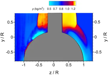
locations: a) x/R=0.4, b) x/R=0.8 and c) x/R=1.0. The regions of high r.m.s. values are observed along the shock structure, shear layers, and boundary layers. Flow is into the page. . . 48 Figure 3.9 Side-by-side comparison of the density field obtained using

cali-brated PLS technique (left half ) and the corresponding computed density field from RANS (right half ). Identical color maps were used on both fields to facilitate quantitative comparison of the experi-mental and computational fields. . . 50 Figure 3.10 Instantaneous and mean profiles of gas density across different

(13)

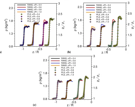
Figure 3.11 Comparison of mean gas density profiles from experiments and RANS simulations across the separation and reattachment shocks obtained at different heights from the cylinder surface. The profiles were obtained at x/R=1.0. . . 54 Figure 3.12 P.D.F. of the experimental density field r.m.s. obtained downstream

of the inviscid shock region between y/R=0.4-0.8 at two different streamwise locations: a) x/R=0.6, and b) x/R=1.0. . . 55 Figure 3.13 Conditionally averaged mean density values downstream of the

inviscid shock, conditioned on the freestream signal counts, at two different streamwise locations: a) x/R=0.6, and b) x/R=1.0. The density data were sampled across y/R=0.4-0.5. . . 58

Figure 4.1 Representation of the (a) fin-on-cylinder and (b) planar fin models used in the experimental investigations. . . 64 Figure 4.2 PLS schematic. . . 67 Figure 4.3 Surface streakline visualization of a 50 mm tall fin on (a) 50 mm

cylinder, and (b) flat plate at Mach 2.5. The black dashed lines are the loci of the first noticeable pressure rise in the surface pressure field obtained from figure 4.4. The dash-dot line is the theoretical location of the inviscid shock. . . 70 Figure 4.4 Unwrapped mean surface pressure field of the (a) fin-on-cylinder

SBLI and (b) planar SBLI. The black dashed line denotes the blue/ -green interface loci that corresponds to the first noticeable surface pressure rise from the SBLI. The dash-dot line is the theoretical location of the invisicd shock. . . 71 Figure 4.5 Freestream-normalized mean wall static pressure profiles. Figure

(a): fin-on-cylinder SBLI, and (b): planar SBLI. . . 73 Figure 4.6 Ensemble-averaged freestream-normalized PLS images at different

streamwise locations: (a)x=20 mm, fin-on-cylinder; (b)x=30 mm, fin-on-cylinder; (c) x =40 mm, fin-on-cylinder; (d) x = 20 mm, planar, and (e)x =30 mm, planar; (f )x =40 mm, planar. Flow is into the page. . . 74 Figure 4.7 Mean PLS freestream-normalized intensity profiles above the

vis-cous region (y =7 mm) at different streamwise locations. . . 76 Figure 4.8 (a) comparison of the freestream-normalized density field at x

= 30 mm acquired via RANS (left half ) and PLS (right half ) and (b) RANS pressure field atx =30 mm downstream (left half ) and proposed schematic of the off-body shock structure in the fin-on-cylinder SBLI configuration (right half ). . . 78 Figure 4.9 Density gradient magnitude contours normalized by the gradient

(14)

Figure 4.10 RANS density gradient magnitude contours normalized by the gra-dient magnitude at fin half-height at (a)x =10 mm, (b)x =20 mm, and (c)x =30 mm. . . 81

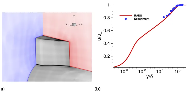
Figure 5.1 Schematic of the test article used for the studies. . . 85 Figure 5.2 Schematic of the PLS setup used for the experiments. . . 88 Figure 5.3 (a) Illustration of the grid generated for the Euler and RANS

simu-lations used in this study. (b) Boundary layer profile comparison between the RANS and the experiment. . . 89 Figure 5.4 Regime map of primary and secondary separation of planar fin

SBLI based on[Zhe82]and the projected regimes of the different fin-on-cylinder SBLI configuraitons used in the current work. . . 92 Figure 5.5 Flow visualizations for each fin angle. This figure contains the flow

vi-sualizations for the following configurations (fin half-angle/ cylinder-diameter/freestream-Mach-number): a) 5◦_/_{76 mm}_/_{M2.5; b) 5}◦_/₇₆

mm/M3; c) 10◦_/_{76 mm}_/_{M2.5; d) 10}◦_/_{50 mm}_/_{M3; e) 10}◦_/_{76 mm}_/_M3;

f ) 12◦_/_{76 mm}_/_{M3; g) 14}◦_/_{76 mm}_/_{M2.5; h) 14}◦_/_{76 mm}_/_{M3; i) 20}◦_/₇₆

mm/M2.5; j) 20◦_/_{50 mm}_/_{M3; k) 20}◦_/_{76 mm}_/_{M3. Flow is from right}

to left. . . 94 Figure 5.6 Unwrapped top-view surface streakline visualization images of

pri-mary separation (S1), pripri-mary reattachment (R1), and secondary separation (S2) loci for combinations of: a) 10◦_/_{50 mm}_/_{3, b) 20}◦_/₅₀

mm/3, c) 10◦_/_{76 mm}_/_{3, and d) 20}◦_/_{76 mm}_/_{3. . . .} ₉₇

Figure 5.7 Top view surface streakline visualization of primary separation (S1), primary reattachment (R1), and secondary separation (S2) loci for a 25-mm tall fin on a) flat plate, and b) 50-mm diameter cylinder at Mach 2.5. . . 98 Figure 5.8 Unwrapped surface mean wall static pressure fields of the

fin-on-cylinder SBLI. The separation and reattachment loci are overlaid from figure 5.7 (b). . . 99 Figure 5.9 Mean wall static pressure profiles along spanwise (for planar fin

SBLI) and azimuthal (for fin-on-cylinder SBLI) direction at different streamwise locations. Figure (a): planar fin SBLI wall pressure pro-files, and (b): fin-on-cylinder SBLI wall pressure profiles. The values are normalized by freestream pressure. . . 101 Figure 5.10 A representative instantaneous PLS field after background

subtrac-tion and laser sheet correcsubtrac-tion obtained at x =25 mm. The flow direction is into the page. . . 104 Figure 5.11 Ensemble averaged freestream normalized PLS images at different

(15)

Figure 5.12 Normalized PLS r.m.s. images at different streamwise locations: (a) x =10 mm; (b)x =15 mm; (c)x =20 mm; and (d) x=25 mm. The abbreviations I.S., S.S., and R.S. refer to Incident Shock, Separation Shock, and Reattachment Shock, respectively. Flow is into the page. 106 Figure 5.13 Simultaneous visualization of surface pressure field and off-body

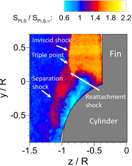
features of the fin-on-cylinder SBLI at: a) x =20 mm, and b)x = 25 mm. . . 108 Figure 5.14 Density fields illustrating the fin-on-cylinder shock structure from

Euler simulations: a) 25-mm tall fin at x=10 mm; b) 25-mm tall fin atx =25 mm; c) infinitely-tall fin atx =25 mm. . . 111 Figure 5.15 Comparisons of inviscid shock density jumps at different

stream-wise locations: a) at y=12.5 mm corresponding to the half-height of the 25-mm tall fin; b) corresponding to the triple point location at different streamwise distances; and c) a comparison between experimental and computed density jumps at y=12.5 mm for the 25-mm fin. . . 113 Figure 5.16 PLS-based density profiles at different streamwise locations at 1 mm

below the triple point. ‘S’ and ‘R’ denotes the locations of separation and reattachment shocks identified from r.m.s. fields. . . 116 Figure 5.17 PLS-based density jump at various y-distances along the

separa-tion shock: (a) density ratio variasepara-tion atx =20 mm along with the corresponding field that illustrates the separation shock structure; (b)y variation of the separation shock strength at different stream-wise locations; (c) corresponding density jump in planar fin SBLI at different streamwise locations. . . 118 Figure 5.18 (a) Off-body PLS-based density field atx =25 mm; and b)

compari-son of the variation of density jump across the separation shock at various heights between 25- and 50-mm tall fins. . . 120 Figure 5.19 Delineation of surface features of the SBLI generated by a 50-mm tall

fin-on-cylinder: a) surface streakline visualization image; b) mean wall pressure field; and c) comparison of freestream-normalized mean wall pressure profiles for the 25-mm and 50-mm tall fins. . . . 121 Figure 5.20 Top view schematics of the separated flow in planar fin SBLI vs.

fin-on-cylinder SBLI to illustrate the separated flow shrinkage down-stream of the limiting boundary layer in fin-on-cylinder SBLI: (a) planar fin SBLI; and (b) fin-on-cylinder SBLI. The shaded orange region portrays the separated flow in both figures. . . 123 Figure 5.21 Surface streakline patterns obtained from RANS simulations of the

fin-on-cylinder SBLI flowfield: (a) without wind tunnel boundary layer interference; and (b) with wind tunnel interference. . . 124

(16)

Figure 6.3 Wake velocity profiles 25 mm downstream of the (a) 3.6mm tall VG and (b) 6 mm tall VG, compared against baseline profiles without the VG. . . 134 Figure 6.4 Baseline pressure field of (a) the cylinder surface and (b) fin face. . 135 Figure 6.5 Percentage changes in fin-normal force and moments with and

without VG control over different VG configurations: (a) normal force on the fin; (b) roll moment; (c) yawing moment; (d) pitching moment. . . 137 Figure 6.6 Flowfield generated by VG: (a) basic schematic of the vortices

gen-erated (reproduced from Yan et. al[Yan17]); (b) surface pressure field over and around the VG; (c) planar laser scattering field of the vortical flow measured 20 mm downstream of VG trailing edge (x= -5mm) . . . 139 Figure 6.7 Mean cylinder surface streaklines: (a) baseline; (b) 6-mm tall VG at

x=-25 mm andφ=-10◦_{; (c) 3.6-mm tall VG at x}₌_{-25 mm and}_φ₌

-10◦; (d) 6-mm tall VG at x=-12 mm andφ=-25◦. . . 140 Figure 6.8 Mean cylinder surface pressures for: (a) baseline; (b) 6-mm tall VG

at x=-25 mm andφ=-10◦_{; (c) 3.6-mm tall VG at x}₌_{-25 mm and}_φ

=-10◦; (d) 6-mm tall VG at x=-12 mm andφ=-25◦. . . 141 Figure 6.9 Mean fin surface pressures for: (a) baseline; (b) 6-mm tall VG at x

=-25 mm andφ=-10◦_{; (c) 3.6-mm tall VG at x}₌_{-25 mm and}_φ₌

-10◦; (d) 6-mm tall VG at x=-12 mm andφ=-25◦. . . 143 Figure 6.10 Cross-section plane z-direction mean velocity field overlaid on the

surface pressure field for: (a) baseline; (b) 6-mm tall VG at x=-25 mm andφ=-10◦. . . 144 Figure 6.11 Incoming boundary layer velocity profile for the 6 mm tall VG placed

90 mm upstream of the fin leading edge. . . 145 Figure 6.12 Mean surface pressure fields for: (a) baseline; (b) 6-mm tall VG at x

=-90 mm andφ=0◦_{. . . 146}

Figure 6.13 Mean surface streaklines for: (a) baseline; (b) 6 mm VG placed atx =-25 mm andφ=0◦; (c) 6 mm VG placed atx=-25 mm andφ=-25◦148 Figure 6.14 Mean surface pressure fields for: (a) baseline; (b) 6 mm VG placed

atx =-25 mm andφ=0◦_{; (c) 6 mm VG placed at}_x ₌_{-25 mm and}

φ=-25◦ . . . 149 Figure 6.15 Mean velocity fields for: (a) baseline, plane:x =-5 mm; (b) 6 mm

VG atx =-25 mm andφ=0◦_{, plane:}_x ₌_{-5 mm; (c) 6 mm VG at}_x

=-25 mm andφ=-25◦, plane:x=-5 mm; (d) baseline, plane:x = 15 mm; (e) 6 mm VG atx=-25 mm andφ=0◦_{, plane:}_x ₌_{15 mm;}

(f ) 6 mm VG at x =-25 mm andφ =-25◦_{, plane:} _x ₌_{15 mm, (g)}

baseline, plane:x =25 mm; (h) 6 mm VG atx =-25 mm andφ=0◦, plane:x =25 mm, (i) 6 mm VG atx =-25 mm andφ=-25◦_{, plane:}

x =25 mm . . . 151

(17)

Figure A.3 Dimensioned drawing of the 20◦_{half-angle fin used in the}

experi-ments. . . 174 Figure A.4 Dimensioned drawing of the 50 mm outer diameter cylinder used

(18)

CHAPTER

1 INTRODUCTION

1.1 Motivation and Goals

Shock interactions with turbulent boundary layers have ubiquitous occurrence in high

speed air platforms, and shock-induced boundary layer separation is the dominant cause

for several undesirable phenomena like scramjet inlet unstart, premature failure of control

surfaces, and roll/side-force reversal in ammunitions, among others. Due to their

impor-tance, shock wave/boundary layer interactions (SBLI) and shock-induced flow separation

have been extensively investigated over the last several decades. Much of the progress made

over the last several decades are reviewed in many articles:[Dol01],[Set94],[Cle14], and

[Gai15].

(19)

ramps[Set76; And87; Van18], sharp fins[Kni87; Kub82], and impinging shock interactions

[Pip09; Hum09; Sou10]. etc. with canonical turbulent boundary layers. Among the different

geometries, SBLI generated by a sharp fin has a direct relevance to control forces and

mo-ments generated in supersonic air vehicles, projectiles and munitions. Almost all previous

studies on fin SBLI were made in planar configurations where the fin is placed on a flat plate

[Kni03; Dol01; Zhe06; Gai15]. Despite this extensive research, it is unclear if the conclusions

drawn are directly extendable to a sharp fin placed on a cylindrical surface, a geometry

common among modern high-speed projectiles and vehicles.

This study is inspired by answering whether the non-linear shock interactions with a

perturbed boundary layer that develops over an axisymmetric body can be used to generate

control forces required for high maneuverability. Such perturbed boundary layers may

come as a result of canard interactions with the tail fin, induced cross-flow from

non-zero incidence flights or unsteady maneuvers, or the introduction of new control surfaces

near the fin root. Specifically, the goal to provide a basic understanding of the underlying

fluid dynamics when a sharp fin is placed on a cylindrical surface to introduce 3-D relief

into the flow. As evident by the literature, little attention has been given to fins placed on

axisymmetric bodies, and even fewer on how that flowfield responds when the incoming

boundary layer is perturbed.

The path taken in this study is multi-fold: first, a new experimental technique was

developed that provides density fields of the body flow to understand how the

off-body flow corresponds to any changes seen in the surface flow when the fin is placed on

a cylindrical surface. This technique is in the form of quantitative planar laser scattering

(PLS). Next, the baseline flowfield is established for the fin placed on a cylindrical surface

in both a pre- and post-separated flowfield. The former allows for direct investigation of

the effect of 3-D relief on the inviscid shock structure, while the latter simulates a post-stall

flowfield that may result from an extreme maneuver while providing rich new physics in

(20)

layer of the baseline flowfield is then perturbed to unravel the non-linear change in the

shock/boundary layer interaction. Thus, this work has the potential to greatly enhance the

aerospace community’s understanding of shock/boundary layer dynamics by providing the

field with a method to visualize a region that is normally challenging in the context of many

SBLI studies, an understanding of how the well-documented planar sharp fin flowfield is

altered when placed in realistic configurations, and potentially insight into ways that can

be used to reduce undesirable phenomena such as control-force reversal or to establish

new control techniques for high maneuverability.

1.2 Literature Review

1.2.1 Review of the Flowfield Past a Sharp Fin

In some of the earliest works, Bogdonoff’s group[Tan87; Bog89; Set80]made wall pressure

measurements to investigate appropriate scaling parameters. They found that the incoming

boundary layer displacement thickness, which is used in 2-D closed separations, is not

an appropriate parameter to scale “open” separations: this was the first indication of the

possible absence of the relevant length scale for this type of separation.[Set85]and[Set86]

examined the pressure fields of the SBLI generated by sharp fins and cones, and showed

that the SBLI unit exhibited quasi-conical symmetry, meaning the statistical properties of

the unit are relatively constant along radial lines originating from a virtual conical origin

(VCO). They also showed that the cone vertex angle (measured with respect to the freestream

direction) resulted in a good agreement in the mean and root-mean-square (r.m.s.) pressure

profiles. Subsequent works by Gibson & Dolling[Gib91]and Schmisseur & Dolling[Sch94]

showed that the power spectrum of the wall pressure fluctuations also collapsed along a

given cone vertex angle.

Accurate prediction of the onset of shock-induced flow separation onset in sharp-fin

(21)

the separation data over several fin- and ramp-induced SBLI, and collated his data with

several other separation data in literature spanning a wide range of Mach numbers and

shock strength. He showed that the shock strength (quantified by inviscid pressure ratio)

that causes separation in 2-D ramp-SBLI has a Mach number dependence. In contrast,

separation in the 3-D fin-SBLI occurred when the inviscid pressure jump across the shock

exceeded the upstream pressure by 50% without a Mach number dependence. While several

subsequent works showed agreement with Korkegi’s separation criterion, many works also

reported a Reynolds number dependence on separation onset.

To address some of the dependence of the state of incoming boundary layer on

separa-tion, free interaction theory (FIT) argued that the shear forces within the boundary layer

subjected to an adverse pressure gradient will help overcome the pressure forces. Using

the momentum balance close to the wall, a relation between the wall pressure beneath the

separation point and the inflow properties was derived. This relation was further used to

de-termine the shock strength corresponding to separation onset. The free interaction theory

was also extended to 3-D planar fin SBLI to predict separation onset and the static pressure

beneath the primary separation[Bab11]. Several efforts showed that the FIT predictions

work quite well at low and moderate Reynolds numbers. Subsequent efforts developed

empirical relations and corrections to FIT to predict the separation onset with much better

accuracy at high Reynolds numbers and in more complex geometries. Babinsky & Harvey

[Bab11]have compiled several of these studies and their regimes of application.

Once the flow is separated, further increase in fin shock strength is reported to

pro-duce interesting flowfields that correlate with the shock strength. Zheltovodov[Zhe82]

characterized different regimes of separation based on the fin shock strength and Mach

number. Using his nomenclature, these regimes are classified as: (I) interaction without

boundary layer separation, (I I) interaction with boundary layer primary separation (and

no secondary separation), (I I I) flow with secondary separation, (I V) secondary

(22)

of secondary separation. For a given Mach number, increasing the fin angle transitions

the SBLI regimes fromI throughV I. Thus, post separation, further increase in the shock

strength causes the generation of additional set of separation and reattachment, called

secondary separation (regimeI I I). An illustration of the flowfield is shown in figure 1.1.

This secondary separation is characterized by a secondary separation vortex that is

generated by the outer flow that is recirculated from the leading edge of the primary

sepa-ration vortex (close to the fin root). However, with increasing shock strength, the velocity of

recirculated flow from the leading edge increases into the turbulent regime, which is more

resistant to separation[Bab11]. This was suggested to cause the suppression and

disappear-ance of the secondary separation (regimesI V andV), which was corroborated by[Zhe87].

Subsequently, the investigation done by[Bal16a]on the effect of Reynolds number on the

sharp fin SBLI resulted in flow patterns largely consistent with the regimes demarcated

by Zheltovodov. The only exception is the case for a freestream Mach number of 3 and a

fin deflection angle of 22◦where Baldwin et al.[Bal16a]noticed the presence of secondary

separation, despite this test case falling within regimeV. Interestingly, the experimental

results modeled by Horstman deviate in the same way for a freestream Mach number of

3.95 and a 20◦_{sharp fin}_[_Hor89_]_{. With further increase in shock strength, recirculating flow}

velocity exceeds sonic conditions and a normal shock forms at the recirculating flow that

causes the re-emergence of the secondary separation (regimeV I).

Significant computational efforts were also undertaken by several researchers to

pre-dict the complex flow structure and surface pressure patterns under various conditions.

These include the RANS simulations by several different groups, as reviewed by Knight

et al.[Kni03], Thivet[Thi02], and more recently by Gaitonde[Gai15]and LES simulations

of Fang et al.[Fan17], Touber & Sandham[Tou09]and Loginov et al.[Log06]. While most

turbulence models used for the RANS simulations provided a reasonably accurate

predic-tion of the onset of primary separapredic-tion, they showed severe discrepancy with experiments

(23)

standard turbulence models could predict the secondary separation that were

experimen-tally observed. A weakly nonlinear extension of thek−ωmodel[Wil88]due to Durbin

[Dur96]predicted the secondary separation with significantly better fidelity compared to

the standard models[Zhe06]. Upon closer investigation, it was shown that the success of

the revised model in predicting the secondary separation onset coincided with a smaller

turbulence kinetic energy within the primary separation vortex and the shear layer above

the vortex. Thus, the secondary separation is determined by the turbulence features of the

primary separation vortex, and, perhaps, the entrainment characteristics of the shear layer.

Alvi & Settles[Alv92]provided excellent qualitative visualization of the off-body flow/

shock structures associated with open separation generated in Regime III using conical

shadowgraphy and planar laser scattering. A schematic of the separation unit based on

their findings is illustrated in figure 1.1. It can be observed from figure 1.1 that the inviscid

shock bifurcates into aλ-shape when it interacts with the boundary layer. The boundary

layer separates behind the upstream stem of theλ-shock to form a primary separation

vortex and subsequently reattaches behind the downstream stem of theλ-shock, and the

size of this open separation scales with the shock strength (i.e. fin angle and incoming Mach

number). Furthermore, the primary streamwise vortex extends from the line of primary

separation S1 to primary reattachment R1. A slipstream emanating from the triple point

of theλ-shock impinges upon the plate near the root of the fin that causes a sharp rise in

the unsteady pressure loading near this impingement location. A sufficiently high velocity

reverse flow was also created underneath the primary separation vortex, which results in

a region of secondary separation, bounded by the separation and reattachment points

S2 and R2, respectively. The experimental findings were also corroborated by RANS and

LES simulations employing different turbulence models[Kni87]and using more advanced

(24)

(a) (b)

Figure 1.1Sketch ofλ-shock structure: (a) streamwise and (b) top views, based on[Alv92].

1.2.2 Planar Laser Scattering

The ability to visualize and quantify these complex off-body flowfields greatly enhances the

understanding of the flow interactions in practical situations and can help advance high

fidelity predictive tools. Several previous methods have been devised and implemented

in the past to visualize different types of flows. Maltby[Mal62]discusses the utilization

of various smoke techniques (such as kerosene vapors) in low speed tunnels but notes

that it is difficult to produce an adequate amount of smoke for high speed flows. For

higher speed flows, specifically those in the supersonic regime, shadowgraph and schlieren

techniques are preferred due to their ability to easily deduce wave structures caused by

density gradients.

Focused schlieren techniques, in particular, have been used successfully to investigate

and quantify complex flows such as boundary layers and wind tunnel noise[Par12],

low-speed axisymmetric mixing layers[Alv93], and the turbulent structures and convection

velocities of supersonic boundary layers[Alv93; Gar98]. Coupled with other systems such

as deflectometers, focused schlieren can be used to acquire turbulence frequency data

via fluctuating density gradients. Although focused schlieren provides a promising,

non-intrusive and cost-efficient method of flow measurement[Gar98], the technique can be

difficult to setup or adjust[Fis50], and may result in low signal to noise ratios[Gar98; Par12].

(25)

these issues with the proper optical systems. However, these techniques are line-of-sight

integrating methods that cause the three dimensional information in the flowfield to be lost.

The vapor screen method first implemented by Allen & Perkins[All51]utilizes a thin light

sheet to illuminate particles within a flowfield. To alleviate some of the condensation effect

when using global seeding in the flowfield[McG61], local vapor seeding was used such as

that by Settles & Teng[Set83], where only the flow region of interest is seeded instead of the

entire flow.

Over the past few decades, planar laser scattering (PLS) has been utilized to

visual-ize instantaneous flow structures of supersonic flows. Clemens & Mungal[Cle91; Cle95]

employed PLS with ethanol fog as seed particulates to visualize the structures within a

supersonic mixing layer. Using the aerosol coagulation model of Fuchs[Fuc64], Clemens

& Mungal[Cle91]were able to account for the qualitative variations in the PLS signals in

the mixing layer across their measurement domain, which spanned about 30 cm in length.

Subsequently, Alvi & Settles[Alv92]used PLS of ice clusters in the flow to visualize the flow

and shock features generated by the planar fin-shock induced separated flow. Wu & Miles

[Wu00]performed MHz rate PLS using seeded gaseousC O2fog to visualize the flow

dynam-ics in shock boundary layer interactions generated by a compression ramp. The authors

chose seed particles that readily evaporated in the boundary layer and separated flow to

give them an excellent contrast in their visualization images. Subsequently, Thurow et al.

[Thu03]implemented MHz rate PLS to study the turbulent mixing and noise generation

in a supersonic jet exhausting into ambient air. More recently, tomographic PLS has been

developed to visualize the 3-D mixing fields in subsonic jets with immense success[Lei14].

One of the biggest drawbacks of the PLS imaging technique is that its utility had been

restricted to qualitative visualization of the flowfield. Traditionally, quantitative imaging of

flowfields has been performed using gas phase measurement techniques such as Rayleigh

scattering, planar laser induced fluorescence, etc. For example, Shirinzadeh et al.[Shi96]

(26)

Balla[Bal15]made mean density measurements over a cap placed in a Mach 10 flow, and,

more recently, made fluctuating density measurements in the same configuration[Bal16b].

Panda & Seasholtz[Pan99]and Mielke et al.[Mie05]have also used Rayleigh scattering for

making density field measurements to study shock/vortex and shock/shock interactions in

underexpanded jets.

Filtered Rayleigh scattering (FRS) imaging is also a common approach for making

density and pressure field imaging in non-reacting flows[For96]. Boguszko & Elliott[Bog05]

used a scanning FRS approach where the scattering spectrum was obtained to determine

mean temperature, velocity, and pressure fields in supersonic free jets. In addition, Elliot

& Samimy[Ell96]performed filtered angularly resolved Rayleigh scattering (FARRS) and

conventional Rayleigh scattering on an underexpanded supersonic axisymmetric jet for

simultaneous velocity, density, and temperature measurements. More recently, George et al.

[Geo14]investigated the use of a combination of wavelengths in FRS scattering, which can

be used for direct measurements of density, and implemented the approach in supersonic

flows.

Planar laser induced fluorescence (PLIF) has also been used as a tool to visualize

non-reacting flows as well as measuring its gas density and temperature. PLIF of NO and OH has

been used to image qualitative temperature and density variations in high-speed flowfields

present in low[Woo04; Nai09]and high enthalpy facilities[Pal95]. NO PLIF has also been

used in the past for quantifying the NO number density fields in high enthalpy facilities

[Dan99]. More recently, two-photon krypton PLIF was used in an underexpanded krypton

jet to obtain centerline density and temperature profiles and to visualize hypersonic conical

shock structures[Nar11; Lam17].

All of the flow quantification techniques using Rayleigh scattering and fluorescence

imaging place a substantial demand on the laser and detector instrumentation for making

measurements: this poses a significant challenge for making measurements over large

(27)

with modest instrumentation. Planar laser scattering (PLS), on the other hand, requires

significantly smaller laser energies; if the PLS imaging can be made quantitative, it can

potentially overcome the challenges for spatial and temporal scalability. Hence, recent

efforts have been made to image the gas density fields in different supersonic flow

con-figurations using a calibrated PLS approach with synthetic nanoparticles seeded into the

flow[Tia09]. Whereas the potential for this technique has been demonstrated in

super-sonic flows, a systematic understanding of the underlying physics and validation has not

been attempted previously. Furthermore, for more general applications, there is a need

to understand calibrated PLS approaches that use readily available and inexpensive seed

materials.

1.2.3 Axisymmetric Geometries with a Sharp Fin

Compared to planar fin SBLI, only a few studies exist for axisymmetric configurations.

Axisymmetric fin SBLI studies like those of Blair et al.[BJ83]focused on determining the

integrated forces on missile-like models[Fre11; Sil15; Sah90; Bha14]. The phenomena of

pitch and roll reversals were reported in these studies when the fin angles exceed stall

angles, wherein further increases in fin angles result in diminished forces and moments.

Most subsequent efforts focused on canard and tail fin interactions to predict and control

the pitch and roll reversal phenomena (e.g.,[Sah17; DeS02]) without emphasizing the

shock-induced flow separation. The works of Hooseria & Skews[Hoo15; Hoo17]have provided

deeper insight into 3-D diffraction of shock waves on curved surfaces when two slender

bodies are placed in close proximity in supersonic flow. These works show the retention of

primary and secondary boundary layer separation on the curved surface, suggesting the

planar regimes set forth by Zheltovodov may be retained for curved geometries.

Bhagwandin[Bha15]performed the only available investigations into the fundamental

features of SBLI generated by an incident oblique shock on a cylindrical surface. The author

(28)

direct incidence on the cylindrical surface versus the circumferential locations where the

shock wave made a grazing incidence like a fin shock. While Bhagwandin’s and Hooseria &

Skews’ studies show the rich flow physics associated with an impinging shock on a cylinder

surface, it is not directly extendable to the SBLI generated by a sharp fin placed on the

cylindrical surface as the impinging inviscid shock structure is substantially different from

that generated by a fin mounted on a cylinder surface.

1.2.4 Perturbed Sharp Fin SBLI

One of the key technological advancements that most projectiles would seek to have is

the ability to make sudden and dramatic turns, which would help achieve very high strike

precision and mitigate collateral damage. The additional and ideal requirements for

im-plementing any desired flow control strategy is that the actuator footprint be small, and

the power requirement fairly minimal. A number of candidate methods have been tested,

prominent among them being the thrust vectoring control jets to cause the sharp turns.

Interestingly vortex based methods have attracted only minimal interest, perhaps due to

very complicated flowfield generated by the vortex generators or due to the fact that the

interactions between the canard wake vortex and the tail fins mainly result in adverse effects

such as roll and pitch reversals[DeS02]. However, the main advantage of the vortex based

methods is the non-linear nature of the flow and the small and simplistic implementation

of the flow actuators. This motivated the current work’s investigation into the flowfield

generated by the tail fins before and after stall (pre- and post-separation) with the rationale

of using vortex control methods on tail fins to create sharp control forces and moments to

engender precision maneuverability.

Previous works have shown that inducing vorticity into the incoming boundary layer

can have significant effects on the SBLI, a review of which is provided by Lu et al.[Lu11]. As

described in this review, the usage of a vortex generator (VG) entrains high momentum fluid

(29)

This reduction in separation size is accomplished by decreasing the boundary layer losses

and producing a considerably healthier (lower shape factor) boundary layer[McC93]. In the

majority of these studies, a closed separation was considered with the goal of controlling

separation by reducing its size[McC93; Bab09; And06; Yan17]. Although these goals were

accomplished and the extent of separation was reduced, the effect of the VG remained

relatively localized. By creating an array of VGs, a spanwise modulation in the shock wave

was seen[Gie14]and the effectiveness of reducing the separation size was increased at the

cost of increasing the disturbance footprint. It remains unclear, however, if these results are

directly extendable to an open separation (i.e. a sharp fin) wherein the underlying flowfield

is different from a closed separation.

When the vorticity induced by the VG interacts with the separation shock of aλ-shock

structure, the result can be a significant distortion or even disappearance of the separation

shock[Lu11]. If separation remains, Martis et al.[Mar14]showed a reduction in its size

and apparent vortex/shock and vortex/vortex interactions evident by aberrations in the

fin SBLI separation structures. Alvi’s group recently showed that the flow response in a

planar fin SBLI configuration depends on the location of the perturbation with respect to

the interaction[Mea18; Mea19]. It was found that perturbing the flow near the inception

region with a jet has a significant effect on the separation and reattachment regions of the

flow. Moving the perturbation location farther downstream reduces the effect at primary

separation and increases it near secondary separation; ultimately, the location of the

in-viscid and separation shocks upstream are shifted with little effect on the pressure field

when the flow is perturbed in conically-symmetric flow. Therefore, the flowfield response

can be controlled by changing the location of a perturbation with respect to the fin leading

edge (inception region), where the SBLI is most sensitive. This result is significant because

it suggests that the bulk of the separation can be modified rather than a localized region

and the effectiveness of the VG can propagate further downstream in an open separation,

(30)

1.3 Technical Approach

To investigate the effect of 3-D relief on a sharp fin SBLI, a myriad of experimental techniques

are employed to analyze both the surface and off-body mean flows of a fin placed on a

cylindrical surface. Oil flow streaklines provide a qualitative picture of the shear contours

and separation entities, while pressure sensitive paint (PSP) provides a quantitative picture

of the surface pressure field. Moreover, planar laser scattering (PLS) and particle image

velocimetry (PIV) are used to determine how the off-body flow corresponds to the patterns

seen on the surface. A technique was developed to calibrate the PLS intensity fields to

density fields to enhance its quantitative value, thus providing deeper insight into the

physics at play. When possible, all processing is done with in-house codes developed in

MATLAB; the notable exception being processing of the velocity fields, which was done in

DaVis 8.4. Because extreme maneuvers of vehicles would represent a wide range of shock

strengths, separation regimes, and distortion magnitudes, extensive work is presented in

this manuscript in which the Mach number, fin angle, extent of 3-D relief, and perturbation

size are varied. Complementary planar fin SBLI and computational RANS simulations are

presented as well as a basis of comparison to the fin-on-cylinder configuration and to

extend the results into regions unobtainable in the experiments. A consolidated list of all of

the experimental and computational methods is provided in chapter 2.

1.4 Problem Context

Before discussing the details of the experiments, it is important to illustrate the uniqueness

of the flow configuration studied to show that fin SBLI over a cylindrical surface (or any

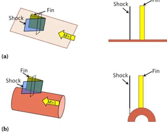
curved surface) is not a simple extension of planar fin SBLI. Figure 1.2 considers an inviscid

supersonic flow over an infinitely tall fin placed on a flat plate (figure 1.2 (a)) and on a

(31)

(a)

(b)

Figure 1.2Illustration of fundamental modifications to the inviscid shock structure generated in a fin-on-cylinder configuration.

distance for the two cases (shown as a dashed rectangle) is compared for the two cases.

It can be observed that for the planar case, the inviscid shock wave retains its strength

and shape across the fin height all the way to the plate surface. In contrast, for the case of

fin mounted on a cylindrical surface, the inviscid shock of a constant strength will extend

across the fin height; however, the shock strength cannot be supported in the region close

to the cylindrical surface (shown as dashed line) as there is no compression surface. This

modifies the inviscid shock structure and features in the region close to the cylindrical

surface. The 3-D relief of the cylindrical surface described in this manuscript denotes the

additional room along the azimuthal direction offered to the flow due to the curvature of

the cylinder surface. For now, it is important to note that even the inviscid shock system

generated by the fin mounted on a cylindrical surface is quite different from the planar

case. The incoming boundary layer reacts to the adverse pressure gradient caused by the

modified inviscid shock, resulting in interesting outcomes to the SBLI flowfield that are

(32)

1.5 Overview of Dissertation

Chapter 2 outlines the experimental and computational setups used in the subsequent

analyses.

Chapter 3 outlines the novel technique of turning the normalized PLS intensity fields

into normalize density fields. The theory behind this analysis is presented, as well as a

discussion on the expected error magnitudes. The results show excellent agreement with

corresponding RANS simulations, and is a promising technique for investigating the

devel-opment of the off-body shock structure.

Chapter 4 isolates the effect of 3-D relief on a sharp fin SBLI that is unseparated, which

corresponds to mild maneuvers and interaction strengths. Because the flow is unseparated,

the influence of 3-D on the inviscid shock structure can be directly analyzed. A significant

weakening of the shock is seen in the vicinity of the cylinder surface–a phenomenon not

present in planar geometries–and an analysis of the modified shock structure is provided.

Chapter 5 extends the analysis of the baseline mean flowfield for when a sharp fin is

placed on a cylindrical surface. An investigation of the influence of interaction strength and

extent of 3-D relief on the separation regimes and entities is provided, with special interest

given to a highly separated (post-stall) flowfield. A significant deviation from a planar fin

SBLI is seen in the size and growth rate of the separated flow, and the shock structure is

shown to exhibit a unique curvature as a result of finite fin height effects and 3-D relief.

Having established the baseline flow structure, chapter 6 investigates the effect of

introducing streamwise vorticies into the incoming boundary layer on the mean flowfield.

Various sizes of micro-ramp vortex generators are used to simulate varying perturbance

strengths that would be introduced from upstream control surfaces or maneuvers. An

analysis of the relevent mechanisms and perturbation locations provides promising support

for exploiting the non-linear shock interactions for enhancing vehicle control forces.

(33)

for future work.

1.6 Published Works

The research provided in this dissertation led to the publication of the following works.

1.6.1 Journal Papers

1. Pickles, J. D., Mettu, B. R., Subbareddy, P. K., & Narayanawamy, V. “On the mean

structure of sharp-fin-induced shock wave/turbulent boundary layer interactions

over a cylindrical surface”.Journal of Fluid Mechanics865(2019), pp. 212 – 246.

2. Pickles, J. D., Mettu, B. R., Subbareddy, P. K., & Narayanawamy, V. “Gas density field

imaging in shock dominated flows using planar laser scattering”.Experiments in

Fluids59.12 (2018), pp. 1 – 15.

3. Pickles, J. D. & Narayanawamy, V. “Investigation of Surface Curvature Effects on

Unsep-arated Fin Shock Wave/Boundary Layer Interactions”.AIAA Journalto be published

(2019).

4. Pickles, J. D. & Narayanawamy, V. “Achieving High Maneuverability and Precision in

Munitions Using Non-Linear Flow Interactions”.AIAA Journalunder review(2019).

1.6.2 Conference Papers

1. Pickles, J. D., Mettu, B. R., Subbareddy, P. K., & Narayanawamy, V. “Fin-generated

shock wave/turbulent boundary layer interactions on a cylindrical surface with a

distorted incoming boundary layer”.AIAA Aviation 2018 Forum. American Institute

(34)

2. Pickles, J. D., Mettu, B. R., Subbareddy, P. K., & Narayanawamy, V. “Sharp-fin induced

shock wave/turbulent boundary layer interactions in an axisymmetric

configura-tion”.47th AIAA Fluid Dynamics Conference. American Institute of Aeronautics and

Astronautics. 2017. pp. 1 – 21.

3. Pickles, J. D., Mettu, B. R., Subbareddy, P. K., & Narayanawamy, V. “Sharp-fin induced

shock wave/turbulent boundary layer interactions in an axisymmetric

configura-tion”.46th AIAA Fluid Dynamics Conference. American Institute of Aeronautics and

Astronautics. 2016. pp. 1 – 19.

4. Lam, K-Y, Pickles, J. D., Narayanawamy, V., Carter, C. D., & Kimmel, R. L. “High-Speed

Schlieren and 10-Hz Kr PLIF for the new AFRL Mach-6 Ludwieg Tube Hypersonic Wind

Tunnel”.55th AIAA Aerospace Sciences Meeting. American Institute of Aeronautics

and Astronautics. 2017.

5. Pickles, J. D. & Narayanawamy, V. “Achieving High Maneuverability and Precision in

Munitions Using Non-Linear Flow Interactions”.31st International Symposium on

Ballistics. International Ballistics Society.to appear 2019. pp. 1 – 12.

6. Mettu, B. R., Pickles, J. D., Subbareddy, P. K., Narayanawamy, V., Vasile, J. & DeSpirito, J.

“Analysis of turbulence models to predict fin-on-cylinder shock boundary layer

(35)

CHAPTER

2 INVESTIGATION METHODS

In this chapter, an overview of the experimental and computational conditions are provided

for each of the methods used in this study. Although a general description of the PLS setup is

described here, Chapter 3 is dedicated to describing the theory and research into developing

the technique.

2.1 Experimental Approach

2.1.1 Wind Tunnel Facility

All experiments were performed in the supersonic wind tunnel facility at North Carolina

State University. This is a blowdown tunnel with a variable throat design to achieve test

(36)

that vents into ambient air on the roof of the laboratory building. The test section has a

constant area measuring 150 mm_×150 mm_×650 mm. Optical access to the test section

is provided via a 100 mm circular port on the tunnel ceiling and two removable quartz

windows on the sides. Models can be mounted on either the tunnel ceiling or either sidewall

via customizable mounts which replace the circular plug or windows, respectively. In this

way a variety of camera angles and imaging planes can be used to acquire data as required.

Moisture is removed from the freestream air (compressed into two large tanks at 930 kPa)

via a drying unit manufactured by Ingersoll-Rand, which maintains a dew point of at least

230 K. The dryer can also be partially bypassed to control the amount of moisture present in

the freestream when conducting PLS experiments. The tunnel is controlled via a LabView

VI that is programmed to alter the tunnel run time and stagnation pressure as needed. The

VI is also equipped with a PID controller that maintains a constant stagnation pressure for

the duration of the run. For most experiments, a run time of 6 seconds was used.

2.1.2 Models

A hollow half-cylinder model (annular cross-section) made of low carbon steel, 430 mm

long, was machined to have a sharp leading edge and was placed facing the freestream at

nominally zero yaw and pitch angle with respect to the incoming flow (figure 4.1 (a)). The

half-cylinder model spanned a full 180◦_{and had an outer diameter of 50 mm. For a subset}

of the experiments, a cylinder model of similar specifications but a 76 mm outer diameter

was used. A sharp fin was mounted on the cylinder surface at a downstream distance of

340 mm to create a shock wave that would interact with the boundary layer that developed

on the cylinder surface. A standard right-hand coordinate system was defined at the fin

leading edge/fin root with positivexin the streamwise direction and positivey pointing

vertically outward along the fin.

Complementary investigations were also performed in a planar fin SBLI configuration

(37)

those of a canonical planar fin SBLI (figure 4.1 (b)). The planar fin SBLI was generated by a

20◦_{sharp fin that was mounted to a 370 mm long flat plate in Mach 2.5 flow. A boundary layer}

developed over the plate surface and transitioned naturally to fully developed turbulent

boundary layer. The fin was mounted such that its leading edge was located approximately

270 mm downstream of the plate leading edge, and the plate’s mounting struts recessed the

unit away from the wind tunnel wall boundary layer. A summary of the incoming boundary

layer characteristics is shown in table 6.1. Comparison of the entries in table 1 shows that

the boundary layer parameters are quite similar between the fin-on-cylinder and planar

fin SBLI geometries, allowing for direct comparison between the two configurations. A

schematic of the two configurations with the origins defined is shown in figure 4.1.

(a) (b)

Figure 2.1Representation of the (a) fin-on-cylinder and (b) planar fin models used in the experimental investigations.

For most experiments presented in this work, the fins were 25 mm in height, which was

approximately a factor of four taller than the incoming boundary layer thickness. However,

isolated studies were made using another 50 mm tall fin for certain fin angles to explore

the effect of fin height on the SBLI. Two half-cylinder models with outer diameter of 50 mm

and 76 mm were employed for this study, and fin half-angles ofα= 5◦_{, 10}◦_{, 12}◦_{, 14}◦_{, and}

(38)

Table 2.1Incoming flow and boundary layer characteristics

Parameter Fin-on-cylinder SBLI Planar fin SBLI

xB L 290 mm 245 mm

M∞ 2.5 2.5

u_∞ 580 m/s 580 m/s

T_∞ 130◦_K ₁₃₀◦_K

Re/m 5.3_×107_/_m _5.3_×₁₀7_/_m

Re_θ 15000 17000

δ99 6 mm 5 mm

θ 0.28 mm 0.31 mm

Cf 0.0017 0.0020

a factor of 2.7 to 4 smaller than the different half-cylinder model radii. The fins made a

line contact with the cylinder surface, and the maximum gap between the fin root and the

cylinder surface was less than 1 mm. Additional experiments were performed in which

the fin was contoured to the cylinder surface, and no detectable changes were seen in the

results.

2.1.3 Freestream Conditions

All experiments were conducted at nominally constant stagnation pressure and

temper-ature of 450 kPa and 300 K, respectively. Further, most experiments were at a freestream

Mach number of 2.5. These conditions resulted in a freestream unit Reynolds number of

approximately 5.3 x 107_/_{m and a freestream temperature of 140 K, using isentropic} rela-tions. A boundary layer developed over the cylindrical and planar surfaces that naturally

transitioned to a fully developed equilibrium turbulent boundary layer, as verified with a

van Driest II transform of the boundary layer velocity profile[Hop72]. A summary of the

incoming boundary layer characteristics at Mach 2.5 is provided in table 6.1. The different

(39)

2.1.4 Measurement Techniques

2.1.4.1 Surface Streakline Visualizations

Surface streakline visualizations (SSV) of the separated flow caused by the fin SBLI were

performed for all experimental configurations. To perform the visualization, the test model

was painted with a mixture of UV-fluorescent pigment (DayGlo T13 “Rocket Red” pigment)

and mineral oil before the experimental run. As the wind tunnel stream flowed over the

model during the test run, the dye mixture was driven by the flow shear to result in

streak-line patterns that provided a qualitative picture of the local shear stress. The dye mixture

accumulated at the regions of low shear stress because of the lack of a driving shear force,

allowing for the identification of separation loci. While the streaklines appear to converge

at the (primary and secondary) separation loci, a distinct line from which the streaklines

diverge identifies the reattachment loci. In this manner, a qualitative view of the separated

flow topology can be obtained. The convergence and divergence of the streaklines were

determined by obtaining a movie of the dye flow during the experimental run at 60 fps

using a Nikon D5200 DSLR camera. A 50 mm f/1.2 lens was used, filtered with a 600 nm

longpass filter. The visualization quality was enhanced by illuminating the measurement

region using an 20 W UV lamp, which yielded stark fluorescence signals from the dye that

contrasted well with the black cylinder surface.

2.1.4.2 Mean Pressure Imaging

The surface pressure fields of the SBLI were imaged using pressure sensitive paint (PSP)

from ISSI Inc. The manufacturer reported this paint to have a sensitivity of 0-200 kPa with

a 300 ms response time and low temperature dependence. A 20 W UV lamp was used

to illuminate the paint, and images were captured at 60 fps with a 12-bit CMOS camera

(Photron, Model: FASTCAM SA-X2) longpass filtered at 600 nm. In-house calibration of

(40)

Because the PSP experiments were performed separate from the PLS studies, calibration was

done with dry air to match the freestream conditions under normal operating conditions of

the dryer (a minimum dew point of appropriately 230 K). However, no significant difference

in calibration was obtained using atmospheric air. Therefore, the water droplets used in

PLS have no influence on the uncertainty of the PSP contained herein. Should an intense

water fog be present in the freestream during the experiment, calibration should be redone

to improve accuracy as the water droplets may scatter/absorb the UV light, causing an

under-prediction in PSP intensity (over-prediction in pressure). The mean pressure field

was computed using approximately 200 images with an imaged spatial resolution of 250

µm/pxl.

As a statement of the error in the pressure imaging, the pressures during calibration

were monitored to within 1%, which would linearly translate to an error of 1% in the PSP.

Moreover, the relative standard deviation of the 200 images was found to be approximately

3% across the entire region of interest. At high azimuthal angles (|s|>30 mm), errors can

be found upwards of 10%; therefore, these regions have been excluded from any analysis.

This error can be alleviated, however, by imaging the side of the cylinder. Comparing

multiple data sets across several days, a deviation of roughly 7% was seen globally. This

error is attributed to slight variations in stagnation conditions, spatial resolutions, and

consistency of the coat of PSP on the model surface. The day-to-day variation seen in the

results, however, was a global shift in the pressure values and did not change the trends

(and thus conclusions) contained in this manuscript. Thus the errors within the PSP are

estimated to be within 10% of their true values, without an expected change in the trends

or conclusions drawn.

2.1.4.3 Planar Laser Scattering

Planar laser scattering (PLS) imaging was performed in wall-normal/spanwise (y −z)

(41)

flow structure, as shown in figure 2.2. The dew point of the air stream was controlled via

the dryer unit that supplied air to the storage tanks. The low temperature conditions of the

freestream caused the introduced vapor to condense/freeze into a droplet/ice fog, allowing

for the identification of the flow features from the large scattering signals. The intensity of

the scattering directly trends with the local density since regions of higher density result

in a larger seeding density. Elevated temperatures in the viscous regions (near wall) cause

diminished signals due to particulate melting and evaporation, limiting the application

of this technique to the inviscid regions of the flow. A 10 Hz Nd-YAG laser was used to

illuminate the fog with approximately 30 mJ of energy per pulse. Images were recorded at

83µm/pxl with a CCD camera (PCO Tech, Model: Pixelfly) fitted with 105 mm f/2.5 lens

and 532 nm bandpass filter.

To correct for variations within the laser profile, the background-subtracted PLS images

were normalized by the freestream signals in each row of the image. Because the seeding of

the water vapor was homogeneous, quantitative gas densities within the SBLI were able to be

computed from the PLS images. This technique as well as an extensive uncertainty analysis

is described in detail in chapter 3. In summary of the error, the different streamwise locations

contained in this manuscript under similar conditions showed a maximum systematic error

of 3% and a precision error of approximately 8% in the mean density due to uncertainty

in the calibration, laser energy fluctuations, and variations in water concentration. It is

expected that the errors are of a similar magnitude in this analysis. Approximately 120

images obtained from three separate runs were use to compute statistical information of

the normalized PLS image.

2.1.4.4 Particle Image Velocimetry

The off-body velocity fields were measured using particle image velocimetry (PIV).

Ap-proximately 180 images spanning 6 runs were acquired using a CCD camera (PCO Tech,

Sharp-Fin Induced Shock Wave/Turbulent Boundary Layer Interactions over a Cylindrical Surface.

ABSTRACT

DEDICATION

BIOGRAPHY

ACKNOWLEDGEMENTS

TABLE OF CONTENTS

LIST OF TABLES

LIST OF FIGURES

CHAPTER

1

INTRODUCTION

1.1

Motivation and Goals

1.2

Literature Review

1.2.1

Review of the Flowfield Past a Sharp Fin

1.2.2

Planar Laser Scattering

1.2.3

Axisymmetric Geometries with a Sharp Fin

1.2.4

Perturbed Sharp Fin SBLI

1.3

Technical Approach

1.4

Problem Context

1.5

Overview of Dissertation

1.6

Published Works

1.6.1

Journal Papers

1.6.2

Conference Papers

CHAPTER

2

INVESTIGATION METHODS

2.1

Experimental Approach

2.1.1

Wind Tunnel Facility

2.1.2

Models

2.1.3

Freestream Conditions

2.1.4

Measurement Techniques