A Statistical Comparison of Reference Evapotranspiration Methods: A Case Study from Jharkhand State of India

(1)

ISSN: 2319-8753

International Journal of Innovative Research in Science,

Engineering and Technology

(An ISO 3297: 2007 Certified Organization)

Vol. 3, Issue 1, January 2014

Copyright to IJIRSET www.ijirset.com 8765

A Statistical Comparison of Reference

Evapotranspiration Methods: A Case Study

from Jharkhand State of India

Swati Pandey

1

, Manoj Kumar

2

, Soubhik Chakraborty

3

and N.C. Mahanti

4

1,3,4

Department of Applied Mathematics, BIT, Mesra, Ranchi- 835215, Jharkhand, INDIA

2_{Deptt. of Environmental Sciences, Central Univ. of Jharkhand, Brambe, Ranchi-835205, Jharkhand, INDIA}

3_{Corresponding author S. Chakraborty}

ABSTRACT: Agricultural planning relying on evapotranspiration suffers due to inaccuracy in its estimation. The

non-availability of meteorological parameters required for accurate estimation of reference evapotranspiration (ETo) resulted in the development of different methods of ETo estimation. The present study compares various universally accepted methods of ETo estimation by considering the Penman Monteith as a standard method. Comparative analysis indicated the suitability of Hargreaves (1985) method followed by Christiansen (1968) method and Pan Evaporation method (1977). The improvement in ETo estimation was carried out through transformation of standard equations using single or multi parametric approach after analyzing dependency and sensitivity of different meteorological parameters on ETo. The developed transformed models indicated that during ETo estimation morning time relative humidity (RH1) can play the dominant role (99%). ETo estimation by combination of bright sunshine hours and wind speed (WV) exhibit better role (98.8%) than the combination of minimum temperature (Tmin) and WV (98.6%).

Keywords:Evapotranspiration, statistics, transformed model, meteorological parameters

I. INTRODUCTION

(2)

ISSN: 2319-8753

International Journal of Innovative Research in Science,

Engineering and Technology

Reference evapotranspiration (ETo) provides a standard crop (a short, clipped grass) with an unlimited water supply so that a user can calculate maximum evaporative demand from that surface for a given day. This value, adjusted for a particular crop, is the consumptive use (or demand), and deficit represents that component of the consumptive use that goes unfilled, either by precipitation or by soil-moisture use, during the given time period. This deficit value is the amount of water that must be supplied through irrigation to meet the water demand of the crop [2]. The field based direct measurement of ETo by using Lysimetric method, though very much accurate, cannot be used everywhere because of high cost involved in installation and maintenance of lysimeter. Therefore computation of reference evapotranspiration with available meteorological data is one of the important tasks for irrigation planners, researchers to design storage reservoir, which can give the maximum benefit.

In search of the best ETo model for wide application, many researchers ([14]; [11]; [3]; [20]; [18]; [4]; [16]; [15]) have compared different evapotranspiration models. Penman-Monteith equation gives the best estimate of ETo where daily weather data are available [12]. This method is also reliable in a wide range of environments [1].

However, no single existing method using meteorological data is universally adaptable under all climatic regimes. Large number of data requirement also limits the application of many of these methods.

As per the estimates given by the United Nations and World Bank [5] about 70% of the world food demand towards 2025 will be provided through irrigated areas. Therefore for the efficient management of irrigation water, the proper computation of ETo at micro level is highly essential.

The erratic rainfall and high evapotranspiration rate in some parts of the Jharkhand state render such areas highly vulnerable to drought during the southwest monsoon. Therefore it is essential to understand the spatial and temporal variability of the amount of rainfall received in relation to evapotranspiration rate in order to develop effective water management strategies to combat drought in these regions.

In the present study, the authors attempted computation of ETo for a dry semi humid region of Jharkhand, on similar lines as proposed by [16] for semi arid region in Gujarat state of India. Additionally model comparison and validation was done based on error estimation by computing root mean square error (RMSE), percentage error (PE), coefficient of variation (CV), coefficient of determination (R2) and F test. Considering the Penman-Monteith method as a standard method, the regression equations were developed using various meteorological parameters. The resultant regression equations, which have lower values of R2 were transformed to develop improved regression models. The results of the present work demonstrated the validity of different models along with the importance of meteorological parameters both individually and collectively in deducing ETo.

II. MATERIAL AND METHODS CLIMATIC DATA AND STUDY AREA

(3)

ISSN: 2319-8753

International Journal of Innovative Research in Science,

Engineering and Technology

SELECTION OF METHODS FOR ETO ESTIMATION

The primary choice for selection of a particular method for estimation of ETo depends primarily on the degree of accuracy needed and the availability of meteorological parameters. The various methods used by earlier workers for estimation of ETo include Pan Evaporation method (EP), Thornthwaite method (TW), Hargreaves method (HM), Turc method (TC), Christiansen method (CM), Modified Penman method (MP), Makkink Radiation method (MR), FAO Blaney Criddle method (FBC) and Penman Monteith method (PM). The formulation of these methods are given as under

Pan evaporation method (Doorenboss and Pruitt 1977)

p pan

o

E

K

ET



where,

E

_pan = pan evaporation in mmday-1

_K

_p = pan coefficient

For the Class A evaporation pan, the

_K

_p varies between 0.35 and 0.85. Average

_K

_pan = 0.70

T

Thhoorrnntthhwwaaiittee mmeetthhoodd (1948)

a

I T L

ET0 1.6 (10 / ) where, L is the day length factor and is calculated by possible hours of sunshine. I is the annual heat index and is determined as I = Σi, monthly heat index values, i, obtained from 1.514

)

5 /

(

T

a

i



; a is exponential

constant

Hargreave method (Hargreave and Somani 1985)

5 . 0 ) 8 . 17 (

0023 .

0 R TC TR

ETo  a  where,

R

a= extra terrestrial radiation (Lyday

-1_);

m in m ax

T

TR





. (°C);

TC

= mean temperature (°C)

T

Tuurrcc mmeetthhoodd ((11996688))

where,

ET

_p= mean daily potential evapotranspiration

(mm/day);

R

_s= daily global solar radiation (kJ/m2/day);

T

_a = mean daily air temperature (°C).

Christiansen method using pan evaporation (1968, 69)

S H W T

pan

C

E

ET



0 .

755

where,

E

_pan is measured pan evaporation, and the C terms are dimensionless coefficients for temperature (T), mean wind speed (W), mean relative humidity (H) and percent of bright shunshine hours (S).

Modified Penman method (Doorenboss and Pruitt 1977)

where:

ET

_o reference evapotranspiration [mm day-1],

R

_n net radiation at the crop surface [MJ m-2 day-1], G soil heat flux

(4)

ISSN: 2319-8753

International Journal of Innovative Research in Science,

Engineering and Technology

vapour pressure [kPa],

e

_a actual vapour pressure [kPa],

e

_s



e

_asaturation vapour pressure deficit [kPa], ∆ slope vapour

pressure curve [kPa °C-1], γ psychrometric constant [kPa °C-1].

Makkink Radiation (1957)

12 .

0

5 .

58

61 .

0 _



















R

s

ET



where,

R

s is in equivalent energy units, ly day -1_{, and}

ET

is in mm/day.

In a new calibration, Doorenbos and Pruitt (1977) shows an adaptation of the Makkink method as:

12 .

0

5 .

58

61 .

0 _



















s rg

R

ET



, where, a and b are empirical factors which account for relative humidity and daytime

wind movement.

ET

and

R

s

/



are in mm/day.

FAO-24 Blaney-Criddle method (Doorenbos and Pruitt, 1977)

d d rg

U

RH

a

N

n

RH

a

U

a

N

n

a

RH

a

b

N

n

RH

a

T

p

f

bf

a

ET

m in 5 m in 4 3 2 m in 1 0 m in

/

41 .

1 /

0043

.

0 )

13 .

8

46 .

0 (

















where,

ET

_rgis reference crop

ET

in mm/day, p is the percent of daytime hours for a single day compared to the day

length of an entire year, T is the average temperature in degree Celsius, n/N is measured sunshine divided by possible

sunshine,

RH

_{m in}is minimum relative humidity in percent,

U

_d is daytime wind speed in m/s.

Penman-Monteith method (1965)



















ET

.

H

C

p

Q



[

e

0T_z



e

_z

]

/

r

_a _,

H

R

G

n





,

















a c

r

1

*



where, Δ is the slope of the saturation vapour pressure- temperature curve (kPaK-1),



is the psychrometer coefficient

kPaK-1,

C

_p is the coefficient of specific heat for moist ambient air at constant pressure in kJkg-1K-1,

r

_a is known as

aerodynamic resistance in sec/m to the diffusion of water vapor from the evaporating surface, z is measurement elevation in m, and

r

_c is canopy resistance in sec/m.

a

r

h



1 /

where, h is known as the convective heat transport coefficient (Wm-2 K-1).

(5)

ISSN: 2319-8753

International Journal of Innovative Research in Science,

Engineering and Technology

more acceptability of Penman-Monteith method over others, we considered it as a standard method for comparison and validation.

After giving due consideration to the merits and applicability of different methods, ETo were obtained for the study area along with various measures of error estimation viz, CV, PE and RMSE.

The selected method of ETo were then fitted to regression equations with Tmax, Tmin, Tmean, RH1, RH2, RH, WV, BSS, to examine which parameter plays important role in the estimation of ETo. Further the regression equations that were showing lower values of R2 were transformed into the new regression models.

I

IIIII..RREESSUULLTTSSAANNDDDDIISSCCUUSSSSIIOONNSS

COMPUTATION OF DAILY ETO

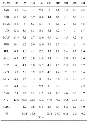
ETo observed by Penman Monteith method was (3.9 mmday-1). The values obtained by Thornthwaite (3.6 mmday-1) and Hargreaves (4.4 mmday-1) methods exhibit proximity to ETovalues obtained from Penman Monteith method. However the ETo computed by Makkink Radiation (2.6 mmday-1) produced underestimated ETovalues whereas Modified Penman (4.9 mmday-1), Christiansen (5.4 mmday-1), FAO Blaney Criddle (6.8 mmday-1) and Pan Evaporation (7.4 mmday-1) methods overestimates ETo values. Turc method (13.5 mmday-1) produced highly overestimated values of ETo.Higher ETo estimates by about 6% using Hargreaves method in comparison to FAO56PM method were reported by [13].

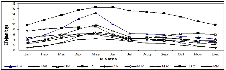
It was observed that the ETo decreases during the months of July, August and September, which comprised the peak monsoon season with high relative humidity, low wind speed and lower temperature [16]. Similar ETo values were observed in the month of November, December and January that comprises the winter season with low temperature causing low evaporation rates as shown in figure 1. In fig 1 it was observed that the values obtained by the turc method were overestimated, however Hargreaves method shows values close to Penman Monteith method. Makkink Radiation produced underestimated ETovalues as compared to the Penman Monteith method.

Lower values ofcoefficient of variation (CV) were obtained during ETo computation by Turc (17.2%) and Modified Penman (19.9%) methods followed by FAO Blaney Criddle (23.5%) and Hargreaves (27.4%) methods. Penman Monteith (30.1%) and Christiansen (37%) methods yielded relatively higher CV values whereas Pan Evaporation (42.6%), Makkink Radiation (43.6%) and Thornthwaite (55.9%) methods produced significantly higher CV values. The high CV values in these methods are due to the significant influence of total sunshine hours, wind speed and humidity. The RMS error was lowest in Christiansen (2.3 mmday-1) and FAO Blaney Criddle (2.7 mmday-1) methods whereas its highest values were obtained while using Makkink Radiation and Turc method (5.2 and 6.4 mmday-1 respectively). The Percentage Error (PE) was lowest in Christiansen (25.4%) and Modified Penman (27%) methods. In remaining methods PE values were quite high (37.5% to 64.6%). However in FAO Blaney Criddle and Turc method the PE values were negative i.e –2.5% and – 99.4% respectively. Very high PE in some of the methods could be due to wide variation of input meteorological parameters, which are significantly related to the ETo estimates. The values of CV, PE, RMSE calculated for various methods are given in table 1.

SENSITIVITY OF DIFFERENT METHODS OF ETO

(6)

ISSN: 2319-8753

International Journal of Innovative Research in Science,

Engineering and Technology

(R2=28.1%) method produced substantially lower R2 values. The value of F test revealed that in all the select methods the values were significant, except in the case of FAO Blaney Criddle method with F value of 3.91 as compared to its table value of 4.84 at 5% level of significance.

SENSITIVITY OF METEOROLOGICAL PARAMETERS FOR DEVELOPED MODELS

Individual meteorological parameter has its own contribution towards ETo. These parameters in isolation and in combination cause different magnitude of evapotranspiration [10]. [21] determined the ETo as a function of temperature f(T), temperature and relative humidity f(T,RH), temperature, relative humidity and wind speed f(T,RH,WV), temperature, relative humidity, wind speed and sunshine hours f(T,RH,WV,BSS) using the Penman-Monteith method and found that in most of the cases the combination of T,RH,WV,BSS shows significant results. Therefore in the present study the effect of individual meteorological parameter was also studied in isolation and in combination to deduce different sets of equations for estimation of ETo. We selected Penman Monteith method to derive the regression equations with Tmax, Tmin, Tmean, RH1, RH2, RH, WV, BSS. Therefore ETo was estimated by selecting one, two, three and four parameters as given in the equation below.

One parameter

(1) ETo= 0.266 Tmax -3.84 R2 = 94.0%

(2) ETo= 0.132 Tmin+ 1.62 R

2

= 43.1%

(3) ETo= 0.206 Tmean-1.04 R2 = 69.2%

(4) ETo= -0.102 RH1+12.1 R2 = 54.9%

(5) ETo= -0.0206 RH2+ 4.91 R2 = 8.9%

(6) ETo= -0.0438 RH + 6.71 R

2

= 20.4%

(7) ETo= 0.655 WV+ 0.853 R2 = 52.7%

(8) ETo= - 0.010 BSS+ 3.96 R2 = 0.0%

Two parameters

(9) ETo= 0.282 Tmax - 0.069 WV- 4.00 R 2

= 94.3% (10) ETo= 0.0150 Tmin + 0.596 WV+ 0.87 R2 = 52.9% (11) ETo= 1.08 WV + 0.451 BSS - 4.36 R2 = 86.0 (12) ETo = 0.220 Tmean - 0.0524 RH +2.01 R2 = 98.1%

Three parameters

(13) ETo= 0.206 Tmax + 0.319 WV + 0.201 BSS - 4.99 R2 = 97.8% (14) ETo= 0.217 Tmax + 0.171 WV - 0.0175 RH2- 2.33 R2 = 97.8% (15) ETo= 0.153 Tmin + 0.595 WV + 0.577 BSS-5.63 R2 = 96.6%

(16) ETo =0.200 Tmean - 0.0528 RH + 0.0842 WV+2.13 R2 = 98.3%

Four parameters

(17) ETo= 0.209 Tmax + 0.250 WV - 0.0096 RH2 + 0.097 BSS- 3.56 R2 = 97.9%

(18) ETo= 0.191 Tmean - 0.0349 RH + 0.232 WV + 0.151 BSS- 0.58 R2 = 98.7%

(7)

ISSN: 2319-8753

International Journal of Innovative Research in Science,

Engineering and Technology

RESIDUAL ANALYSIS

The residual of regression model could be examined to see if they provide any indication that the model is adequate or not [9]. The residuals are the differences between what is actually observed, and what is predicted by the regression equation.

The residuals are defined as ei = Yi -



i

Y

, i = 1,2,3…n where Yi is an observed value and



i

Y is the corresponding fitted /

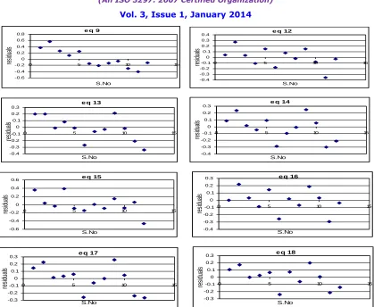
predicted value obtained by use of the regression model. The residuals of different regression equations were plotted in the time order sequence plot (figure 2).

The i-th standardized residual eis is defined as eis = ei /s, where s is the standard deviation of residuals. The standardized residuals eis have zero mean and unit standard deviation. The residuals should be distributed approximately as independent, normal deviates for a large sample [6].

The developed regression equations (1 to 18) were checked for the residual plots and it was observed that some of the equations were showing good scatter plots in the time order sequence (figure 2). Therefore from the entire set of derived equations only some of the equations as 9, 12, 13, 14, 15, 16, 17 and 18 can be selected for accurate estimation of ETo based on their best-fit method.

T

TRRAANNSSFFOORRMMAATTIIOONNOOFFTTHHEEVVAARRIIAABBLLEESS

In regression analysis, a convenient starting point is that the model describing the data is linear in the parameters. The necessity for transforming the data arises because the original variables, or the model in terms of the original variables, violate one or more of the standard assumptions. The most commonly violated assumptions are those concerning the linearity of the model and the constancy of the error variance. When the error variance is not constant over all the observations, the error is said to be heteroscedastic, which can be removed by means of a suitable transformation. The transformation is not only to stabilize the variance, but also have the effect of making the distribution of the transformed variable closer to the normal distribution [6].

While fitting equations to data, [7] was consulted. Regression equations 3, 4, 7, 10 and 11 which produced lower values of R2 were modified by applying suitable transformation. While applying transformation, emphasis was given to improve R2 value which indicates better estimation of ETo.

The new transformed models for the select equations are given below:

(1) Equation (3) ETo= 0.206*Tmean-1.04 (R2= 69.2%) is transformed to

3(a) 1/ ETo = 0.931*1/T + 0.211 R 2

= 97.4% 3(b) log ETo = 0.864*1/T + 0.501 R2 = 96.1%

(2) Equation (4) ETo = -0.102*RH1+12.1 (R2 = 54.9%)

4(a) 1/ ETo = 1.63*logRH1 – 2.81 R2 = 99.6%

4(b) 1/ ETo = 0.924*1/RH1+ 0.240 R2 = 97.3%

(3) Equation (7) ETo= 0.655WV+ 0.853 (R2 = 52.7%)

7(a) 1/ ETo = 1.05*log WV – 0.341 R2 = 97.0%

7(b) 1/ ETo = 0.975*1/WV + 0.0238 R2 = 97.7% (4) Equation (10) ETo= 0.0150 Tmin + 0.596 WV+ 0.87 (R2 = 52.9%)

10(a) 1/ ETo = 1.47* 1/Tmin - 0.0313* 1/WV+ 0.176 R2 = 98.6%

10(b) log ETo = 1.43*1/Tmin - 0.0330*1/WV + 0.468 R2 = 97.5% (5) Equation (11) ETo= 1.08 WV + 0.451 BSS - 4.36 (R2 = 86.0)

11(a) 1/ ETo =1.48*1/WV - 0.0283*1/BSS – 0.0725 R 2

(8)

ISSN: 2319-8753

International Journal of Innovative Research in Science,

Engineering and Technology

The transformed models indicated that while estimating evapotranspiration in terms of individual parameter, relative humidity (RH1) play the highest role (99.6%) followed by wind speed (WV, 97.7%) and mean temperature (Tmean, 97.4%) whereas among the combined parameters combination of Tmin and WV (98.6%) and combination of BSS and WV ( 98.8%) have similar impact on ETo estimation.

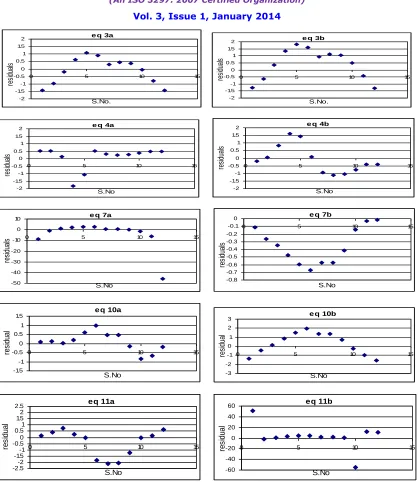
Among the new transformed models shown above, equation 4a shows more positive and few negative points in the plot in comparison to 7b with entire negative points. Equation 7a and 11b shows the entire positive and one negative point. These equations which violate randomness therefore can be rejected as accurate models. The equations 3a, 3b, 4b, 10a, 10b and 11a were showing random plots and therefore can be accepted as models although some pattern points to the requirement of some more parameters in the required model (figure 3). The examination of pattern of scatter plot of new transformed models also suggests that as compared to a single parameter multi-parameters estimation produces better results. It can be remarked that for the estimation of ETo more than two parameters are important, especially Tmean, RH, WV and BSS.

IV. CONCLUSIONS

Regression equations between ETo estimated through Penman Monteith method and other methods indicated that the most significant method of computing ETo is Hargreaves (1985) method (R2=97.2%). This method requires only extra-terrestrial radiation and air temperature data to obtain reliable ETo value and therefore can be applied to regions where data pertaining to other meteorological parameters are not available.

In ETo estimation, Tmax as a single parameter plays prime role, whereas combination of Tmean with RH and Tmax with WV also play significant role. High accuracy in ETo estimation can be achieved by employing three parameters (Tmean, RH, WV) or four parameters (Tmean, WV, RH and BSS)

The developed transformed models indicated that while estimation of ETo, RH1 can play the dominant role (99.6%) followed by WV (97.7%) and mean temperature (97.4%). Combination of BSS and WV (98.8%) exhibit better role than Tmin and WV (98.6%).

Proposed regression equations developed for accurate estimation of ETo:

ETo= 0.282 Tmax - 0.069WV- 4.00 R2 = 94.3% ETo = 0.220 Tmean - 0.0524 RH +2.01 R2 = 98.1% ETo= 0.206 Tmax + 0.319 WV + 0.201BSS - 4.99 R2 = 97.8% ETo= 0.217 Tmax + 0.171WV - 0.0175RH2- 2.33 R

2

= 97.8% ETo= 0.153 Tmin + 0.595 WV + 0.577 BSS-5.63 R2 = 96.6%

ETo =0.200 Tmean - 0.0528 RH + 0.0842 WV+2.13 R2 = 98.3%

ETo= 0.209 Tmax + 0.250WV - 0.0096RH2 + 0.097BSS - 3.56 R2 = 97.9% ETo= 0.191 Tmean - 0.0349RH + 0.232WV + 0.151BSS- 0.58 R2 = 98.7%

The proposed transformed models for estimation of ETo:

1/ ETo = 0.931*1/T + 0.211 R2 = 97.4% log ETo = 0.864*1/T + 0.501 R

2

= 96.1% 1/ ETo = 0.924*1/RH1+ 0.240 R2 = 97.3%

1/ ETo = 1.47* 1/Tmin - 0.0313* 1/WV+ 0.176 R2 = 98.6%

log ETo = 1.43*1/Tmin - 0.0330*1/WV + 0.468 R2 = 97.5%

1/ ETo =1.48*1/WV - 0.028*1/BSS – 0.0725 R 2

= 98.8%

(9)

ISSN: 2319-8753

International Journal of Innovative Research in Science,

Engineering and Technology

The study demonstrated the usefulness of statistical techniques for validating the reference evapotranspiration values obtained by using different EToestimationmethods. The inaccuracies in EToestimations are a major hindrance in developing effective water management strategies for maintaining crop water requirement during drought periods. Therefore application of developed models of evapotranspiration estimation proposed in the study can also benefit toward drought mitigation based on reliable ETo estimates in data scarce region of Jharkhand state.

ACKNOWLEDGEMENTS

Authors are thankful to Prof. A Wadood, Birsa Agricultural University (BAU), Ranchi for providing meteorological data. Authors are also thankful to Dr. M.K. Khandelwal, Principal Scientist, Central Soil Salinity Research Institute, Bharuch (ICAR) for his valuable inputs during the manuscript preparation.

REFERENCES

[1] Allen, R. G., Smith, M., Perrier, A., and Pereira, L. S., “An update for the definition of reference evapotranspiration”,ICID Bulletin, Vol. 43, pp.1-34, 1994.

[2] Allen, R. G., Pereira, L. S., Raes, D., and Smith, M., “Crop evapotranspiration guideline for computing crop water requirements”, FAO Irrigation and Drainage, Rome, Italy, Vol. 56, 1998.

[3] Al-Shan’lan, S. A., and Salih, A. M. A., “Evapotranspiration estimates in extremely arid areas”, J. Irrigation and Drainage Engineering, Vol. 113(4), pp.565-574, 1987.

[4] Amatya, D. M., Skaggs, R. W., and Gregory, J. D., “Comparison of methods for Estimating REF-ET”, J. Irrigation and Drainage Engineering ASCE, Vol. 121(6), pp.427-435, 1995.

[5] Anonymous., “More irrigation needed to meet 21st_{century food needs”, Int. Water Irri., Vol. 20(2), pp.6, 2000.} [6] Chatterjee, S., and Price, B., “In Regression Analysis by Example”,Wiley, New York, 1977.

[7] Daniel, C., and Wood, F. S., “In Fitting equations to data”, John W Sons, New York, 1979.

[8] Doorenbos, J., and Pruitt, W. O., “Crop water requirements”, FAO Irrigation and Drainage, Rome, Italy, Vol. 24, pp.144, 1977. [9] Draper, N. R., and Smith, H., “In Applied Regression Analysis”, John W Sons, New York, 1981.

[10] Goyal, R. K., “A reference evapotransipiration model for arid region of Rajasthan”,Indian J. of Soil Cons., Vol. 32(1), pp.10-15, 2004. [11] Hargreaves, G. H., and Samani, Z. A., “Reference evapotranspiration from temperature, Applied Engineering in Agriculture”, Transaction, Am. Soc. of Agril. Engg., Vol. 1(2), pp.96-99, 1985.

[12] Hess, T. M., “Evapotranspiration estimates for water balance scheduling in the UK”, Irrigation News, Vol. 25, pp.31-36, 1996. [13] Itenfisuel, D., Elliott, R. L., Allen, R. G., and Walter, I. A., “Comparison of reference evapotranspiration calculation across a range of climate”, Proc. of the National Irrigation Symposium, ASAE, Vol. 14-16, Phoenix, pp.216-227, 2000.

[14] Jensen, M. E., “Consumptive use of water and irrigation water requirement”, American Society of Civil Engineers, pp.227, 1974.

[15] Khandelwal, M. K., and Pandey, V., “Comparison of PET computed by various methods in different agroclimatic stations of Gujarat State”, Journal of Agrometerology, Vol. 2, pp.439- 443, 2008.

[16] Kumar, M., and Pandey, V., “Validation of different evapotranspiration models over semi arid region of India”, Int. J. Math. Model. Simul. Appl., Vol. 1(3), pp.321-327, 2008.

[17] Makkink, G. F., “Testing the Penman formula by means of lysimeters”, Journal of the Institution of Water Engineering, Vol. 11(3), pp.277- 288, 1957.

[18] Mohan, S., “Inter Comparison of evapotranspiration estimates”, Hydrological Science, Vol. 366, pp.447-460, 1991.

[19] Pandey, S., Kumar, M., and Mahanti, N. C., “Evaluating interrelationship of meteorological parameters using regression model: A case study from Ranchi, Jharkhand, India”, Indian J. Soil Cons., Vol. 36(3), pp.136-143, 2008.

[20] Rao, V. U., and Murty, K. P. R. V., “Computing Potential Evapotranspiration by different Methods”, Annals of Arid Zone, Vol. 27(3 & 4), pp.253-261, 1988.

[21] Tilahun, K., “Analysis of rainfall climate and evapo-transpiration in arid and semi-arid regions of Ethiopia using data over the last half a century”,Journal of Arid Environments, Vol. 64, pp.474-487, 2006.

(10)

ISSN: 2319-8753

International Journal of Innovative Research in Science,

Engineering and Technology

MON EP TW HM TC CM MP MR FBC PM

JAN 4.1 0.9 3 9.8 3 4.8 1.2 7.3 2.5

FEB 5.8 1.6 3.9 11.8 4.1 5.5 1.7 8.3 3.4

MAR 8.6 3 5.3 13.7 6 6.1 2.7 8.6 4.5

APR 12.2 5.4 6.3 15.5 8.1 6.2 4.1 9 5.7

MAY 14.4 7.1 6.7 16.6 9.9 6.4 4.5 9.2 6.1

JUN 10.1 6.2 5.6 16.6 7.4 5.7 4.1 6 4.8

JUL 6.5 4.6 4.1 15.2 5.2 3.8 3.4 4.2 3.6

AUG 6.3 4.5 3.9 14.8 5.1 4 2.8 4.7 3.6

SEP 6 4.1 3.8 14.2 4.9 4.5 2.5 5.7 3.7

OCT 5.3 2.9 3.9 12.9 4.3 4.4 2 6.3 3.4

NOV 4.9 1.6 3.3 11.1 3.7 3.8 1.5 6.5 2.7

DEC 4.4 0.9 3 9.9 3.3 3.7 1 6 2.2

Aver 7.4 3.6 4.4 13.5 5.4 4.9 2.6 6.8 3.9

CV 42.6 55.9 27.4 17.2 37.0 19.9 43.6 23.5 30.1

RMSE 4.2 3.6 6.4 2.3 3.4 5.2 2.7 4.0

PE 53.4 37.5

-99.4

25.4 27.0 64.6 -2.5 45.2

(11)

ISSN: 2319-8753

International Journal of Innovative Research in Science,

Engineering and Technology

Copyright to IJIRSET www.ijirset.com 8775 Table 2: Regression coefficients between Penman Monteith (PM) method and other methods

Figure1: Comparison of nine ETo methods for Ranchi

ETo method Intercept slope R2 (%) F test

Pan evaporation (EP) 1.21 0.36 94.6 174.4

Thornthwaite (TW) 2.06 0.51 76.5 32.6

Hargreaves (HM)) -0.31 0.95 97.2 342.4

Turc (TC) -1.99 0.43 73.6 27.9

Christiansen (CM) -0.80 0.57 95.3 203.9

Modified Penman (MP) -0.94 0.97 67.2 20.5

Makkink Radiation (MR) 1.41 0.94 85.4 58.6

(12)

ISSN: 2319-8753

International Journal of Innovative Research in Science,

Engineering and Technology

Figure 2: The residual plots of some of the regression equations in time order sequence. e q 9

-0.6 -0.4 -0.2 0 0.2 0.4 0.6 0.8

0 5 10 15

S.No

re

sid

ua

ls

e q 12

-0.4 -0.3 -0.2 -0.1 0 0.1 0.2 0.3 0.4

0 5 10 15

S.No

re

sid

ua

ls

e q 13

-0.4 -0.3 -0.2 -0.1 0 0.1 0.2 0.3

0 5 10 15

S.No re si du al s

e q 14

-0.4 -0.3 -0.2 -0.1 0 0.1 0.2 0.3

0 5 10 15

S.No re si du al s

e q 15

-0.6 -0.4 -0.2 0 0.2 0.4 0.6

0 5 10 15

S.No re si du al s

e q 16

-0.4 -0.3 -0.2 -0.1 0 0.1 0.2 0.3

0 5 10 15

S.No re si du al s

e q 17

-0.3 -0.2 -0.1 0 0.1 0.2 0.3

0 5 10 15

S.No re si du al s

e q 18

-0.3 -0.2 -0.1 0 0.1 0.2 0.3

0 5 10 15

(13)

ISSN: 2319-8753

International Journal of Innovative Research in Science,

Engineering and Technology

Figure 3: The residual plots of selected regression models after transformation in time order sequence.

e q 3a

-2 -1.5 -1 -0.5 0 0.5 1 1.5 2

0 5 10 15

S.No. re si du al s

e q 3b

-2 -1.5 -1 -0.5 0 0.5 1 1.5 2

0 5 10 15

S.No. re si du al s

e q 4a

-2 -1.5 -1 -0.5 0 0.5 1 1.5 2

0 5 10 15

S.No re si du al s

e q 4b

-2 -1.5 -1 -0.5 0 0.5 1 1.5 2

0 5 10 15

S.No re si du al s

e q 7a

-50 -40 -30 -20 -10 0 10

0 5 10 15

S.No re si du al s

e q 7b

-0.8 -0.7 -0.6 -0.5 -0.4 -0.3 -0.2 -0.1 0

0 5 10 15

S.No re si du al s

e q 10a

-1.5 -1 -0.5 0 0.5 1 1.5

0 5 10 15

S.No

re

si

du

al

e q 10b

-3 -2 -1 0 1 2 3

0 5 10 15

S.No re si du al eq 11a -2.5-2 -1.5-1 -0.50 0.51 1.52 2.5

0 5 10 15

S.No re s id u a l eq 11b -60 -40 -20 0 20 40 60

0 5 10 15