Optimization of Data Density and Energy in Wireless Sensor Network

(1)

Vol. 4, Issue 2, February 2015

Optimization of Data Density and Energy in

Wireless Sensor Network

Lavanya 1, Dhanalakshmi 2, Dhivyanjali 3, Priyanga 4 , Esther 5

U.G. Student, Department of ECE, Dr. SJS Paul Memorial College of Engineering and Technology, Puducherry, India 1

U.G. Student, Department of ECE, Dr. SJS Paul Memorial College of Engineering and Technology, Puducherry, India2

Assistant Professor, Department of ECE, Dr. SJS Paul Memorial College of Engineering and Technology, Puducherry,

India 5

ABSTRACT: Wireless sensor networks consist of sensor nodes with sensing and communication capabilities. We focus on data aggregation problems in energy constrained sensor networks. The main goal of data aggregation algorithms is to gather and aggregate data in an energy efficient manner so that network lifetime is enhanced. In this paper, we present a survey of data aggregation algorithms in wireless sensor networks. We compare and contrast different algorithms on the basis of performance measures such as lifetime, latency and data accuracy. We conclude with possible future research directions. Since sensors have limited lifetime, the need for developing algorithms for aggregating sensors' data forms an important concern in the area of WSNs.

We present W-LEACH, a data-stream aggregation algorithm for WSNs that extends LEACH algorithm. W-LEACH is able to handle non-uniform networks as well as uniform networks, while not affecting the network lifetime. It, instead, increases the average lifetime for sensors. We simulate our algorithm to evaluate its performance. Results show that W-LEACH increases the network lifetime and the average lifetime for sensors for uniform and non-uniform WSNs.

KEYWORDS: Wireless Sensor Network, Data Aggregation, Data Density, Clustering method, W-leach.

I. INTRODUCTION

A Wireless Sensor Network (WSN) consists of spatially distributed autonomous sensor to monitor physical or environment conditions, such as temperature, sound, pressure etc. and to cooperatively pass their data through the network to a main location. The more modern networks are bi-directional; also enabling control is sensor activity. The development of wireless sensor network was motivated by military applications such as battlefield surveillance; today such networks are used in many industrial and consumer applications, such as industrial process monitoring and control, machine health monitoring, and so on.

The WSN is built of “nodes”- from a few to several hundreds or even thousands, where each node is connected to one(or sometimes several) sensors. Each such sensor network node has typically several parts: a radio transceiver with an internal antenna or connection to an external antenna, a microcontroller, an electronic circuit for interfacing with the sensor and an energy source, usually a battery or an embedded form of energy harvesting. A sensor node mighty vary in size from that of shoebox down to the size of grain or dust, although functioning “motes” of genuine microscopic dimensions have yet to be created. The cost of sensor node is similarly variable, ranging from few hundred of dollars, depending on the complexity of the individual sensor nodes. Size and cost constraints on sensor nodes result in corresponding constraints on resources such as energy, memory, computational speed and communications bandwidth. The topology of WSN can vary from a simple star network to an advanced multi-hop wireless mesh network. The propagation technique between the hops of the network can be routing of flooding.

(2)

accurately evaluating the events in the monitored area with the collected data. For this purpose, sensor nodes should be deployed closely. However, this will cause overlapping of sensor nodes’ sensing areas and the spatial redundancy of adjacent sensor nodes’ data [3],[4]. If every sensor node transmits collected data to the sink node, the sensor nodes will consume a large amount of energy. To reduce the amount of transmitted data in a WSN, a great number of correlation-based data aggregation methods have been studied in the literature [5]-[11].

According to the level of sampled data in data aggregation strategy, data aggregation methods are grouped into three classes: data level aggregation, feature level of aggregation and decision level aggregation [12]. Also, based on the aggregation strategy, we can divide the data aggregation methods into three types: in-network query type [5],[13], data compression type[6],[14] and representative type [7],[9],[15],[16]. It will acquire a long time to obtain a reply from WSN in the first type. The second type is of limited effectiveness as it is too difficult. The third type is perceptive to the correlation measurement for sensor nodes.

The major objective of the representative type is selecting a representative sensor node in the neighbourhood and sending its observation to the sink node. Therefore, the relative error between a representative data and its correlated data is a considerable index for evaluating the represented performance.

The energy efficiency of the DDCD clustering method is not always the uppermost in data transmitting process. While in the clustering process, the DDCD clustering method is an energy efficient one. The main goal of data aggregation algorithms is to gather and aggregate data in an energy efficient manner so that network lifetime is enhanced. Wireless sensor networks (WSN) offer an increasingly attractive method of data gathering in distributed system architectures and dynamic access via WSN.

II. LITERATURESURVEY

Wireless Sensor Networks: a Survey on Environmental Monitoring

Traditionally, environmental monitoring is achieved by a small number of expensive and high precision sensing unities. Collected data are retrieved directly from the equipment at the end of the experiment and after the unit is recovered. The implementation of a wireless sensor network provides an alternative solution by deploying a larger number of disposable sensor nodes. Nodes are equipped with sensors with less precision, however, the network as a whole provides better spatial resolution of the area and the users can have access to the data immediately. This paper surveys a comprehensive review of the available solutions to support wireless sensor network environmental monitoring applications

Data Routing in In-network Aggregation in WSN: a Cluster Based approach

Large scale wireless sensor networks (WSNs) consists of many sensor nodes & these networks are deployed in different classes of applications for accurate monitoring, health, environment etc. The sensor nodes equipped with limited power sources. Therefore, efficiently utilizing sensor nodes energy can maintain a prolonged network lifetime. One of the major issues in sensor networks is developing an energy-efficient routing protocol to improve the lifetime of the networks. The proposed approach is a Cluster Based Data Routing for In-Network Aggregation that has some key aspects such as a reduced number of messages for setting up a routing tree, maximized number of overlapping routes, high aggregation rate, and reliable data aggregation and transmission & provides the best aggregation quality when compared to other existing algorithms

Distributed Spatial Clustering in Sensor Networks

(3)

distributed techniques. Furthermore, E-Link performs 10 times better than the centralized algorithm, and 3-4 times better than the distributed alternatives in communication costs. We also develop a distributed index structure using the generated clusters that can be used for answering range queries and path queries. The query algorithms direct the spatial search to relevant clusters, leading to performance gains of up to a factor of 5 over competing techniques.

Coverage in Wireless Sensor Networks: A Survey

Wireless sensor networks are a rapidly growing area for research and commercial development. Wireless sensor networks are used to monitor a given field of interest for changes in the environment. They are very useful for military, environmental, and scientific applications to name a few. One of the most active areas of research in wireless sensor networks is that of coverage. Coverage in wireless sensor networks is usually defined as a measure of how well and for how long the sensors are able to observe the physical space. In this paper, we take a representative survey of the current work that has been done in this area. We define several terms and concepts and then show how they are being utilized in various research works.

III.CLUSTERINGMETHODDESCRIPTION

Data Density Correlation Degree

In a WSN, if a certain number of neighbouring sensor nodes’ data are close to a sensor node’s data; this sensor node can represent its neighbours in the data domain. This representative sensor node is called the core sensor node.

Definition 1: Core sensor node. Let us consider sensor node v has neighbouring sensor nodes. They are respectively v1,

v2…vn. The data object of v is D. Its neighbouring sensor nodes’ data objects are respectively D1, D2... Dn. If there are

N data object in D1, D2... Dn whose distances to D are a smaller amount than ϵ and min Pts ≤ N ≤n then the sensor node

v is called sensor node. Where min Pts is the amount threshold, ϵ is the data threshold.

Instinctively, the larger the N is, the better representative the sensor node v is to those sensor nodes whose data objects are in ϵ-neighbourhood of D. Meanwhile, high attention of the data objects in the ϵ -neighbourhood of D implies that sensor mode v has a high spatial correlation between it and these sensor nodes. Therefore, to determine the representation degree of v to those sensor nodes whose data objects are in ϵ-neighbourhood of D in quantity, we proposed the data density correlation degree as shown in definition 2.

Definition 2: Data density correlation degree. Let sensor node v has n neighbouring sensor nodes which are inside the cycle of the communication radius of v. They are v1, v2...vn, respectively. The data object of v is D, and its neighbouring sensor nodes’ data respectively D1, D2..., Dn. Among these n data objects, there are N data objects whose distance to D is not as much of than ϵ, and min Pts ≤ N ≤n. After that the data density correlation degree of sensor node v to the sensor node whose data objects are in ϵ-neighbourhood of D is as follows.

Sim (i) = (1− ₍ ₎)+a2(1− ∆₎

+ a3(1− )

--- (1)

Where min Pts is the amount threshold. ϵ is the data threshold. d∆ is the distance between D and the date centre of the data objects which are in the ϵ neighbourhood of D. d is the average distance between the N data objects and D. a1+a2+a3=1

If the date density correlation degree of sensor node v is Sim (v) defined by Eq.1, then we can obtain the properties of Sim (v) as.

1) Sim(v) increases with the increase of N, the amount of data objects which are in the ϵ-neighbourhood of D; 2) Sim(v) increases with the increases with decreases of d∆, the distance between D and the data centre of the date

objects which are in ϵ neighbourhood of D;

3) Sim(v) increases with the decreases of d, the typical distance between D and those data objects which are in the ϵ neighbourhood of D;

4) Sim (v) ϵ [0, 1].

(4)

some sensor nodes. In order to demonstrate the strength of data density degree defined by Eq.1.The pseudo code for Sensor Type Calculation, Local Cluster Construction, and Global Represtantive Sensor Node Selection are given below.

STC PROCEDURE:

Input: Data Threshold - ϵ; Amount threshold – minPts; Weights – a1, a2, a3;

Neighbouring Sensor nodes set of Sensor node i – N (i). Output:

Sensor Type – Core sensor nodes or Non-core sensor node;

Two sets of sensor nodes’ ID stored in each sensor node - NodeSetinner (i) and NodeSetouter (i);

Data Density correlation Degree – sim (i)

(Step 1)

for each i; i ϵ V pardo {/* Parallel process for each i*/ Sensor node i is a non-core sensor node, NearNum=0;

NodeSet (i )inner= ɸ, and NodeSet (i )outer=ɸ

for each j: j ϵ N (i) {

if (||d(i) – d(j)|| ≤ϵ) NearNum++; }/*end for*/

if (NearNum ≥ minPts) {

Sensor node i is a core sensor node; Sim(i)=a(1−

( ))+a2(1− ∆

)+ a3(1− )

else

Sim(i) = 0; }/*end if*/ }/*end for*/

(step 2)

for eachs i: i ϵ V pardo {/* Parallel process for each i*/ if (i is a core sensor node) {

for each j: j ϵ N(i) { if (||d(i) – d(j)|| ≤ ϵ)

NodeSet(i )inner={j} UNodeSet(i )inner;

else NodeSet(i )outer={j} UNodeSet(i )outer;

}/*end for*/ }/*end if*/ }/*end for*/

LCC PROCEDURE:

Input:

Sensor Type – Core Sensor node or Non-core sensor node;

Two sets of sensor nodes’ IDs in each sensor node

-NodeSetinner(i) and NodeSetouter(i);

Data Density Correlation Degree- Sim(i)

Output: ClusterSet={ClusterSet(i)| i ϵ V}, DDCD_Set = {DDCDmax(i)| i ϵ V}

/*Send Information*/

(Step 1)

for each j: j ϵ NodeSet(i)inner {

sensor node i sends the packet - (i, -1,Sim(i)) to sensor node j

}/*each for*/ }/*each for */

if (sensor node i is a non-core sensor node) { for each : j ϵ N(i) {

sensor node i sends the packet - (i, 0,Sim(i)) to sensor node j;

}/*end for*/ }/*end if*/ }/*end for*/

/*Receive Information*/

/*Receive_Packet ID is the first byte of sent packet in Step 1*/

/*Receive_Packet. Relationship is the second byte of sent Packets in Step 1*/

/*Receive_Packet.Sim(i) is the third byte of sent packets in Step 1*/

(Step 2)

for each i: i ϵ V pardo {/*Parallel process for each i*/ DDCDmax(i)=(i, Sim(i))

for each j: j ϵ Nodesetinner(i) {

if Sim(j )> Sim(i)

DDCDmax(i) = (j, Sim(j)),

}/*end for*/

if sensor node i is a core sensor node Cluster Set(i) = NodeSet(i)inner;

if Receive_Packet.relationship==1

ClusterSet(i)={receivePacket.ID}U Cluster Set(i) }/*end for*/

GRS PROCEDURE:

Input: clusterSet = {ClusterSet(i) | i ϵ V} DDCD_Set = {DDCD max(i) | i ϵ V}

/* DDCD max(i) = (ID(i), simmax(i)) */

Output: Representative Sensor Nodes

(Step 1)

for each i: i ϵ V pardo {/* Parallel process for each i*/

if DDCD max(i).ID ≠i{ for each j: j ϵ ClusterSet(i) {

Sensor node i sends DDCD max(i) to sensor node j; }/*end for*/

}/*end if*/ }/*end for*/ IterativeFlag=0;

(5)

MaxSim=max(DDCDmax(j).

Simmax(j)|j=ClusterSet(i)})

MaxID = {j| DDCD max(j),simmax(j)-MaxSim}

if DDCD max(i).ID≠MaxID { DDCD max(i) = (MaxID,MaxSim); IterationFlag=1;

}end /*end if*/ }/*end for*/ If IterationFlag==1

goto (1.2); else stop.

IV.METHODOLOGIES

The different Methodologies used here are

 Setting up Network Model

 Base station and agent selection Module

 Data Communication Module

 Data Density Correlation Degree Module

 Energy Efficient Module

Setting up Network Model

Our first module is setting up the network model. We consider a large-scale, homogeneous sensor network consisting of resource-constrained sensor nodes. Analogous to previous distributed detection approaches; we assume that an identity-based public-key cryptography facility is available in the sensor network. Prior to deployment, each legitimate node is allocated a unique ID and a corresponding private key by a trusted third party. The public key of a node is its ID, which is the essence of an identity-based cryptosystem. Consequently, no node can lie to others about its identity. Moreover, anyone is able to verify messages signed by a node using the identity-based key. The source nodes in our problem formulation serve as storage pointswhich cache the data gathered by other nodes and periodically transmit to the sink, in response to user queries. Such network architecture is consistent with the design of storage centric sensor networks.

Base Station and Agent Selection Module

Our Second Module is Base Station and Agent Selection Module.

BASE STATION

 Base station has computer and sensor database to store collected sensor data MOBILE SINK

 Mobile sink travels in the sensing area and collects data from each sensors

 Upload the collected data to the base station

Data Communication Module

Our Third Module is Data Communication Module. In this module the followings functions are takes place.

 End to end data communication

 When a node needs connection broadcast the request.

(6)

Data Density Correlation Degree (DDCD) Module

Our Fourth Module is Data Density Correlation Degree (DDCD) Module. By using this module the cluster based approach is established. Using this cluster based approach the cluster head aggregates the raw data then the aggregated data are sent to the sink.

Energy Efficient Module

Our Fourth Module is Energy Efficient Module. In this Module the following functions are takes place.

• Energy saving –W-LEACH Algorithm.

• Neighbours go to sleep when there is no transmission.

• Reduces the traffic load and conserve energy of the sensors.

V. W-LEACH OR WEIGHTED LEACH

W-Leach is a centralized algorithm. As LEACH, an algorithm operates in cycles so that each tower should have two phases, namely a setting phase and a steady state phase. In the configuration phase, W-LEACH selects a number of sensors to be CHs. Each CH is selected based on a weight value which corresponds to each node. Unlike LEACH, whether a sensor is CH or not in the preceding rounds, is independent in W-LEACH. After all CHs are selected clusters are formed such that each sensor is assigned to its closest CH. Leach requires each CH collects data from all sensors in its group at its steady state phase, against W-Leach chooses only x% of sensors in each group to send data to their CH. Candidates for sending data to CHs are selected according to their weight.

Although the W-LEACH protocol has advantages in terms of an energy recovery but this protocol is based on knowledge of the location of nodes to select the nodes between transmission nodes and nodes remain in sleep. In addition it does not consider the mobility of sensor nodes after the "installation phase" of groups in a round while the W-LEACH protocol accompanies a lot of data loss in mobility environment focused on "hot spots". Because its application is limited to nodes fixed sensors.

In our work the W-LEACH WITH BECON RESPONDER outperforms W-LEACH in terms of environment, field of use in underground and Mobility to extended Network lifetime. W-LEACH BECON RESPONDER is based on a number of neighbors to reorganize node density after that it selects active nodes and those which remain asleep in a BECON RESPONDER manner. After the text edit has been completed, the paper is ready for the template. Duplicate the template file by using the Save As command, and use the naming convention prescribed by your conference for the name of your paper. In this newly created file, highlight all of the contents and import your prepared text file. You are now ready to style your paper; use the scroll down window on the left of the MS Word Formatting toolbar.

Weighted LEACH: it’s an extended LEACH to challenge uniform and non-uniform network. In set up phase, the base station based on density of nodes to divide member nodes in two groups. One group member nodes transmit their data while the member nodes in the other group remain asleep. The selection of nodes which remain asleep is centralized. Weighted Low Energy Adaptive Hierarchy (W-LEACH) is an extension of LEACH to efficiently handle non-uniform sensor distribution in WSNs. It increases the lifetime of the network. But this protocol is centralized because the base station is the only responsible for selecting sleeping nodes and active nodes. In addition, the base station needs the location node to manage the density of nodes after it informs each node with an additional traffic. In this paper, we propose later a BECON RESPONDER algorithm which weighs LEACH without nodes’ maps.

WEIGHTED LEACH:

1. Proposes clustering of sensors + cluster leaders.

(7)

 Rotating cluster head balances energy consumption.

 Cluster formation distributed and energy efficient. 2. Time is divided into rounds.

3. A node self-elects itself as the cluster head.

4. Higher residual energy, higher probability to be head.

 Close-by sensors join this cluster-head.

 Cluster head does TDMA scheduling and gathers data.

 Gathered data compressed based on spatial correlation.

 Transmits data to Base Station (@ higher power) 5. In the next round, another cluster head elected.

 Probabilistic load balancing.

 Network lifetime can increase manifolds.

The Advantages of W-LEACH are,

 Energy saving:

 Neighbours go to sleep when sense transmissions

 Reduces control overhead by sending multiple data

 With the help of data aggregation process we can enhance the robustness and accuracy of information which is obtained by entire network, certain redundancy exists in the data collected from sensor nodes thus data fusion processing is needed to reduce the redundant information.

 Another advantage is those reduces the traffic load and conserve energy of the sensors.

 Achieves performance superior to existing protocols in terms of energy efficiency, packet delivery ratio (PDR), and latency.

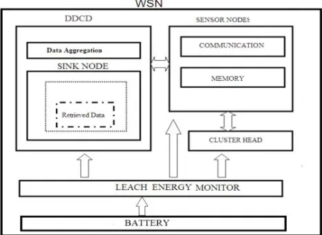
 Simulation results also show better performance than that of two recent proposals for routing around dead ends.

Fig 1. System Architecture of Wireless Sensor Network.

W-LEACH with becon responder algorithm

(8)

transmits there data. Member nodes after receiving they calculate the number of nearest neighbours to a lower maximum distance determined. If this number is less than a limited number the node goes to sleep during this round as N3. Else the nodes calculate their Time Slot to transmit their data as N1dierily.

VI.NS2W-LEACHIMPLEMENTATION

Purpose

What is necessary to install and run the W-LEACH protocol on version 2.35 of ns2? At the time of this writing, this is the newest version of ns2. The WLEACH implementation was written as a stand-alone application. Thus, in the past a version compiled for WLEACH may or may not work for other protocols. In addition, the original version of WLEACH was compiled for version 2.5b which is an outdated version of ns2.

The following goals have been achieved:

 Merged and compiled ns2.35 to support WLEACH protocol.

 Modified code to allow for support of all protocols including LEACH without

 Recompilation.

 Validated running of all demos using the ns2.35.

 Executed LEACH simulation included in the uAMPS changes package (tcl/ex/wireless.tcl)

VII.CHANGESINADDINGW-LEACHSUPPORT

Below is a list of all the line numbers that were changed in existing ns2-35 code. This does not include the addition of the mit directory with additional code.

apps/app.cc:53:#ifdef MIT_uAMPS apps/app.cc:126:#ifdef MIT_uAMPS apps/app.h:53:#ifdef MIT_uAMPS

common/mobilenode.cc:341:#ifdef MIT_uAMPS common/packet.cc:49:#ifdef MIT_uAMPS common/packet.cc:135:#ifdef MIT_uAMPS common/packet.h:63:#ifdef MIT_uAMPS common/packet.h:167:#ifdef MIT_uAMPS common/packet.h:223:#ifdef MIT_uAMPS common/packet.h:404:#ifdef MIT_uAMPS common/packet.h:515:#ifdef MIT_uAMPS common/packet.h:587:#ifdef MIT_uAMPS common/packet.h:610:#ifdef MIT_uAMPS common/packet.h:677:#ifdef MIT_uAMPS mac/channel.cc:117:#ifdef MIT_uAMPS mac/ll.h:55:#ifdef MIT_uAMPS

mac/ll.h:110:#ifdef MIT_uAMPS

mac/mac-sensor-timers.cc:5:#ifdef MIT_uAMPS mac/mac-sensor-timers.h:5:#ifdef MIT_uAMPS mac/mac-sensor.cc:5:#ifdef MIT_uAMPS mac/mac-sensor.h:5:#ifdef MIT_uAMPS mac/mac.cc:95:#ifdef MIT_uAMPS

mac/phy.cc:60:#ifdef MIT_uAMPS mac/phy.h:93:#ifdef MIT_uAMPS mac/phy.h:146:#ifdef MIT_uAMPS

mac/wireless-phy.cc:94:#ifdef MIT_uAMPS mac/wireless-phy.cc:114:#ifdef MIT_uAMPS mac/wireless-phy.cc:133:#ifdef MIT_uAMPS mac/wireless-phy.cc:220:#ifdef MIT_uAMPS mac/wireless-phy.cc:237:#ifdef MIT_uAMPS mac/wireless-phy.cc:373:#ifdef MIT_uAMPS mac/wireless-phy.cc:433:#ifdef MIT_uAMPS mac/wireless-phy.cc:593:#ifdef MIT_uAMPS mac/wireless-phy.h:52:#ifdef MIT_uAMPS mac/wireless-phy.h:116:#ifdef MIT_uAMPS mit/rca/rca-ll.cc:7:#ifdef MIT_uAMPS mit/rca/rcagent.cc:7:#ifdef MIT_uAMPS mit/uAMPS/bsagent.cc:8:#ifdef MIT_uAMPS mit/uAMPS/bsagent.h:8:#ifdef MIT_uAMPS trace/cmu-trace.cc:59:#ifdef MIT_uAMPS trace/cmu-trace.cc:1026:#ifdef MIT_uAMPS trace/cmu-trace.cc:1063:#ifdef MIT_uAMPS trace/cmu-trace.cc:1171:#ifdef MIT_uAMPS trace/cmu-trace.h:60:#ifdef MIT_uAMPS

Special Changes

(9)

Add Interface

The method for implementation of the add-interface method of the TCL object library was extended in the latest version of ns2. This resulted in requiring 3 additional parameters whenever a node wished to add an interface. The following code was added at line of the

mit/uAMPS/sims/becon.tcl file. $node topography $topo if ![info exist inerrProc_] { set inerrProc_ ""

}

if ![info exist outerrProc_] { set outerrProc_ ""

}

if ![info exist becon Proc_] { set becon Proc_ ""

}

# Connect the node to the channel.

$node add-interface $chan $prop $opt(ll) $opt(mac) \ $opt(ifq) $opt(ifqlen) $opt(netif) $opt(ant) \

$topo $inerrProc_ $outerrProc_ $ becon Proc_

VIII.EXPERIMENTALRESULTS

NO.OF PACKETS

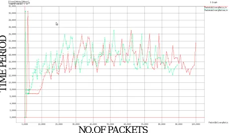
Figure 2: Comparison of Packet Delivery Ratio with DDCD and W-Leach

Figure 2 represents the comparison of packet delivery ratio withW-Leach and DDCD. Here x-axis represents the number of packets and the y-axis represents the time period. DDCD algorithm is represented Red in colour while the greeen colour represents the W-Leach.

NO.OF PACKETS

Figure 3: Comparison of End to End delay with DDCD and W-Leach

Figure 3 represents the comparison of End to End delay with DDCD and W-Leach. Here also the x-axis represents the number of packets and y-axis represnts the time taken to deliver the packets. The graph clearly shows that W-leach takes the less average time to reach the destination when compared to DDCD.

T

IM

E

P

E

R

IO

D

T

IM

E

P

E

R

IO

(10)

NO.OF PACKETS

Figure 4: Represents the Overall Data Density Analization with W-Leach

Figure 4 represents the overall data density analization. Here x axis represents the number of packets and the y-axis represents the time period. The graph shows that the delivery of packets is much faster than the DDCD. And the data density occurs less in W-Leach. Hence it travels faster than the DDCD.

NO.OF PACKETS

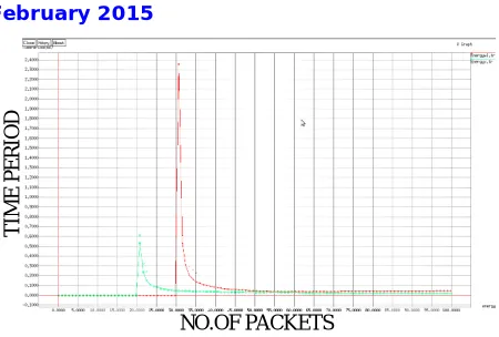
Figure 5: Comparison of Energy Utilization with DDCD and W-Leach

Figure 5 represents the comparison of energy utilization with DDCD and W-Leach. X-axis represents the total number of packets and the y-axis represents the time period. Here the graph shows that the W-Leach consumes less amount of Energy for transmitting the packets when compared to DDCD.

SIMULATION PARAMETERS

Network Dimension 1200*800 m.sq

Number of Nodes 28

Sensor Radius 2 meters

Simulation Time 150 sec

Routing Protocol AODV

Initial Energy 100 joules

Transmission Power 20.500 mwatts

Reception Power 40.119 mwatts

Data Packet 512 bytes

IX.CONCLUSION

The main contributions of this paper are the introduction of the data density correlation degree (DDCD) clustering method. The pseudo code of the DDCD clustering method is given as well. The proposed algorithm provides energy efficient path for transmission and maximizes the life time of a sensor nodes. With the use of DDCD clustering method we can minimize the packet loss ratio and end to end delay. So that the packet delivery ratio has been increased. By using W-LEACH algorithm we can get more energy efficiency.

We have presented comprehensive data aggregation algorithms in wireless sensor networks. All of them focus on optimizing important performance measures such as network lifetime, data latency, data accuracy and energy consumption. Efficient organization, routing and data aggregation construction are the three main focus areas of data aggregation algorithms. We have described the main features, the advantages and disadvantages of each data aggregation algorithm. We have also discussed special features of data aggregation such source coding. The trade-offs between energy efficiency, data accuracy and latency have been highlighted. Most of the existing work has mainly focused on the development of an efficient routing mechanism for data aggregation. However, the performance of the data aggregation protocol is strongly coupled with the infrastructure of the network. There has not been significant

T

IM

E

P

E

R

IO

D

T

IM

E

P

E

R

IO

(11)

research on exploring the impact of heterogeneity and mode of communication on the performance of the data aggregation protocols. Although, many of the data aggregation techniques presented look promising, there is significant scope for future research. Combining aspects such as energy, data latency and system lifetime in the context of data aggregation is worth exploring. A systematic way of the relation between energy efficiency and system lifetime is an avenue of our research. Analytical results on the bounds for lifetime of sensor networks are another area worth exploring. Existing work has provided bounds on lifetime for networks with specific network topologies and source behaviours. It would be interesting to extend this work to more general network topologies.

REFERENCES

1. J. Yick, B. Mukherjee, and D. Ghosal, “Wireless sensor network survey,”Comput. Netw., vol. 52, no. 12, pp. 2292–2330, 2008.

2. L.M. Oliveira and J. J. Rodrigues, “Wireless sensor networks: A survey on environmental monitoring,” J. Commun., vol. 6, no. 2, pp. 1796– 2021, 2011.

3. C. Zhu, C. Zheng, L. Shu, and G. Han, “A survey on coverage and connectivity issues in wireless sensor networks,” J. Netw. Comput. Appl., vol. 35, no. 2, pp. 619–632, 2012.

4. G. Fan and S. Jin, “Coverage problem in wireless sensor network: A survey,” J. Netw., vol. 5, no. 9, pp. 1033–1040, 2010.

5. S. Madden, M. J. Franklin, J. M. Hellerstein, and W. Hong, “TAG: A Tiny AGgregation service for ad-hoc sensor networks,” ACM SIGOPS Operating Syst. Rev., vol. 36, no. 1, pp. 131–146, 2002.

6. J. Zheng, P. Wang, and C. Li, “Distributed data aggregation using Slepian- Wolf coding in cluster-based wireless sensor networks,” IEEETrans. Veh. Technol., vol. 59, no. 5, pp. 2564–2574, Jun. 2010.

7. M. C. Vuran, Ö. B. Akan, and I. F. Akyildiz, “Spatio-temporal correlation: Theory and applications for wireless sensor networks,” Comput. Netw.,vol. 45, no. 3, pp. 245–259, 2004.

8. J. Yuan and H. Chen, “The optimized clustering technique based on spatial-correlation in wireless sensor networks,” in Proc. IEEE Youth Conf. Inf., Comput. Telecommun. YC-ICT, Sep. 2009, pp. 411–414.

9. Rajeswari and P.Kalaivani, “Energy efficient routing protocol for wireless sensor networks using spatial correlation based medium access control protocol compared with IEEE 802.11,” in Proc. Int. Conf. PACC, Jul. 2011, pp. 1–6.

10. J. N. Al-Karaki, R. Ul-Mustafa, and A. E. Kamal, “Data aggregation and routing in wireless sensor networks: Optimal and heuristic algorithms,”

Comput. Netw., vol. 53, no. 7, pp. 945–960, 2009.

11. S. Iyengar, K. Chakrabarty, and H. Qi, “Introduction to special issue on ‘distributed sensor networks for real-time systems with adaptive configuration’,” J. Franklin Inst., vol. 338, pp. 651–653, Jan. 2001.

12. S. Madden, R. Szewczyk, M. J. Franklin, and D. Culler, “Supporting aggregate queries over ad-hoc wireless sensor networks,” in Proc. Mobile 4th IEEE Workshop Comput. Syst. Appl., Oct. 2002, pp. 49–58.

13. R. Cristescu, B. Beferull-Lozano, and M. Vetterli, “On network correlated data gathering,” in Proc. IEEE Comput. Commun. Soc. 23rd Annu. Joint Conf. INFOCOM, Mar. 2004, pp. 2571–2582.

14. M. C. Vuran and I. F. Akyildiz, “Spatial correlation-based collaborative medium access control in wireless sensor networks,” IEEE/ACM Trans. Netw., vol. 14, no. 2, pp. 316–329, Apr. 2006.

15. G. A. Shah and M. Bozyigit, “Exploiting energy-aware spatial correlation in wireless sensor networks,” in Proc. 2nd Int. Conf. Commun. Syst. Softw. MiddleWare, COMSWARE, Jan. 2007, pp.1–6.

16. W. Guo, L. Zhai, L. Guo, and J. Shi, Worm Propagation Control Basedon Spatial Correlation in Wireless Sensor Network. Berlin, Germany: Springer-Verlag, 2012, pp. 68–77.

17. Y. Ma, Y. Guo, X. Tian, and M. Ghanem, “Distributed clustering-based aggregation algorithm for spatial correlated sensor networks,” IEEE Sensors J., vol. 11, no. 3, pp. 641 648, Mar. 2011.

18. M. C. Vuran and O. B. Akan, “Spatio-temporal characteristics of point and field sources in wireless sensor networks,” in Proc. IEEE Int. Conf. Commun., Jun. 2006, pp. 234–239.

19. N. Li, Y. Liu, F. Wu, and B. Tang, “WSN data distortion analysis and correlation model based on spatial locations,” J. Netw., vol. 5, pp. 1442– 1449, Dec. 2010.

20. R. K. Shakya, Y. N. Singh, and N. K. Verma, “A novel spatial correlation model for wireless sensor network applications,” in Proc. 9th Int. Conf.WOCN, Dec. 2012, pp. 1–6.

21. F. Bouhafs, M. Merabti, and H. Mokhtar, “A semantic clustering routing protocol for wireless sensor networks,” in Proc. 3rd IEEE Consum. Commun. Netw. Conf., Jan. 2006, pp. 351–355.