Size Effects in the Analysis of Concrete or Rock Structures

SIZE EFFECTS IN THE ANALYSIS OF CONCRETE OR ROCK

STRUCTURES

.

1)Departamento de Engenharia Mecânica, Universidade Federal de Rio Grande do Sul,Porto Alegre, RS, Brasil. 2)Departamento de Engenharia Civil, Universidade Federal de Rio Grande do Sul,Porto Alegre, RS, Brasil

ABSTRACT

The authors determined numerically the response of geometrically similar reinforced concrete beams built in four different sizes, tested to rupture by Leonhart & Walter (1965) and later reproduced by Ramallo et al (1993), to quantify size effects in reinforced concrete beams. For such purpose the so-called Discrete Element Method (DEM) was employed, modeling the inhomogeneous character of concrete and steel by assuming that their stiffness and specific fracture energies are random fields in 3D-space. The constitutive criteria, based on Hillerborg´s model (1971), presented improvements in the consideration of the spatial correlation of the random fields. The discrete numerical model was also used to reproduce experimental results due to Viet et al (2000) on the influence of sample size on the tensile strength of concrete. In all cases, in order to represent the stress-strain relation for concrete in tension, a bi-linear diagram was resorted to, which proved adequate when the size of the elements is sufficiently small and the inhomogeneous properties of the material are properly accounted for. These conditions require large DEM or FEM models, which cannot be usually employed in engineering practice due to cost-effectiveness considerations. It is shown in the paper that predictions of the failure load of concrete structures, that account for size effects, can be made using larger elements and therefore reduced computational costs, if the appropriate stress-strain relations are adopted. These relations depend both on the size of the element and on the correlation lengths of the random fields that describe the relevant material properties.. The proposed equations were determined by Monte Carlo simulation, using, for the various sizes of structural samples, elements with the same size.

Keywords: Fracture, concrete, size effect, numerical analysis, inhomogeneous materials

INTRODUCTION

Rios & Riera,[1] determined numerically the response of geometrically similar reinforced concrete beams built in four different sizes, tested to rupture by Leonhart & Walter [2]. These tests were later reproduced by Ramallo et al [3]. The numerical analysis employed the Discrete Element Method (DEM), modeling the stiffness and specific fracture energies of concrete and steel as 3D random fields. The approach was also used to reproduce, by Monte Carlo simulation, experimental evidence on the influence of sample size on the tensile strength of concrete due to van Viet et al[4]. This approach allows the simultaneous consideration of the size effect resulting from fracture of the material (Bazant, [5],[6] and the influence of random distribution of relevant properties (Weibull, [7]). In fact, in the present formulation, the DEM requires that random influences, such as the spatial variation of the specific fracture energy of the material, be properly simulated.

It has been shown that when the discrete elements mesh is dense, the shape of the strain softening branch, a straight line in Hillerborg´s model, has marginal influence on the results (Rocha and Riera, [8]; Riera and Iturrioz, [9]; Rios and Riera [1]). However, for structural components subjected to tension or shear or in case of large discrete elements, the effective stress-strain softening branch tends to present the convex shape measured in concrete and mortar samples and numerically simulated by Wittmann et al[10] and Roelfstra and Wittmann [11], who contributed to the understanding of the fracture process in concrete, but did not address the issues of size effects or model invariance. It is clear that the constitutive criteria adopted for an individual element represents a sort of average over a material volume and hence depends on the size of this volume, in other words, on the size of the element. The notion that the parameters needed to describe the behavior of engineering materials under load, actually depend on the size of the elements of the numerical model, is now widely acknowledged. However, the approach has not yet found a place in routine engineering practice on account of several factors, such as the lack of a procedure to evaluate those parameters for elements of arbitrary size.

It must be mentioned that in papers that remained until recently unnoticed by the authors, Rossi and Richer [12] proposed a probabilistic description of the heterogeneous properties and random distribution of micro-cracking to

specific fracture energy. Thus, they imposed no constraint on the energy dissipated by crack propagation. Later, Rossi et al. [13], experimentally assessed size effects on the tensile strength and modulus of elasticity of concrete, while Rossi and Ulm [14] applied the approach to explain the behavior of concrete in compression, also by means of FEM solutions. Fairbairn et al [15] propose a neural network approach to assess material properties at the so-called elementary volume.

It is likewise the purpose of this paper to provide a practical method applicable to the nonlinear fracture analysis of concrete structures of arbitrary dimensions that fail mainly by tension, that is, structures in which sliding with friction does not play a significant role in the failure process.

THE DISCRETE ELEMENT METHOD

The dynamic analysis of samples subjected to tension was performed employing the Discrete Element Method (DEM), which is based on the equivalence between the properties of an equivalent orthotropic elastic continuum and a model made of large numbers of small interconnected uni-axial elements (Nayfeh and Hefzy, [16]. Thus, in the DEM, a continuum is represented by an array of bars able to carry axial loads only, with the mass lumped at the nodes.

(b)

(a)

X'

X Y'

Z

Y

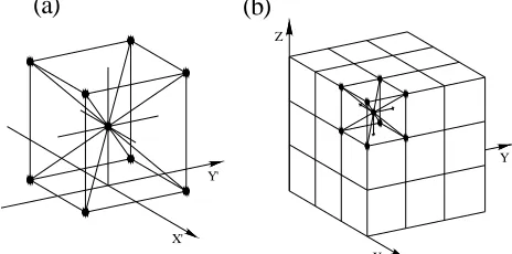
Figure 1. (a) Cubic module and. (b) Prism formed with several cubic modules,

In the cubic array shown in Fig. 1, each node has three degrees of freedom, corresponding to nodal displacements in the three orthogonal coordinate directions. In an isotropic elastic material, the cross-sectional axial stiffness of the longitudinal bars is given by

AEn= φEL, bar length = L, (1)

while for the diagonal bars,

AEd=

3

2

δφEL2_{, bar length =}

2

3

L, (2)

For isotropic solids,

φ

=

(

9

+

8

δ

) (

/

18

+

24

δ

)

δ

ν

(

ν

)

modulus of the material. It is important to point out that for ν = 0.25, the equivalence with an isotropic continuum is complete; while for other values of ν small differences appear in the shear terms, which are herein neglected. It should also be noticed that no lattice or truss-like model can exactly represent a locally isotropic continuum. In fact, no locally isotropic continuum exists. Isotropy in solids is a bulk property that reflects the random distribution of the orientation of constituent elements. Details of the calculation of the equivalent cross-sectional axial stiffness of the normal (AEn) and diagonal (AEd) elements given by equations (1) and (2) can be found in Dalguer et al[17]. The dynamic analysis is performed using explicit numerical integration in the time domain. At each integration step the nodal equilibrium equation (3) is solved by the central finite-differences scheme.

i i

i

c

u

f

u

m

+

=

. ..

, (3)

In eq.(3) m denotes the nodal mass, c a damping constant and

u

u

,

u

the displacement, velocity and

acceleration, respectively, associated with coordinate I, while

f

Figure 2. Bi-linear constitutive relation for fragile material

Riera and Rocha [18] extended the approach to handle fracture by using the bilinear elementary constitutive relationship (ECR) proposed byHillerborg [19] and illustrated in Figure 2(a). This constitutive law aims to capture the irreversible effects of crack nucleation and propagation. The area under the curve corresponds to the energy necessary to fracture the area of influence Af of the element. On the other hand, in compression the material is assumed to remain linear and elastic. Failure of the model, when subjected to compression, is induced by indirect tension (Poisson effect). Constitutive parameters and symbols are shown in Figure 2 (a) and (b).

SIZE-DEPENDENT CONSTITUTIVE LAW

Riera and Iturrioz [20] substituted the bi-linear diagram shown in Fig. 2(b) by a continuous function, using the following expression:

f = a ε exp(- b εc ) ( 0 <ε ) (4)

in which f denotes the stress and a, b and c are constants. The stress times an influence area yields the force in the element. The slope is given by:

df / dε = a ( 1 - b c εc ) exp(- b εc ) (5)

when ε = 0, the stiffness is given by eq.(6), the strain at maximum stress εmax by eq.(7) and the peak stress fmax by eq.(8)

df / dεε= 0 = a , εmax = (b c )-1/ c fmax = a (b c )-1/ c exp [-b (b c)-1/ c ] (6-8)

The unloading branch remains a straight line, as shown in Fig.2(b). The area enveloped by the curve for ε≥0, which defines the work W required for fracturing the element, is given by:

W/Lo = a c-1 b2/cΓ (2/c ) (9)

In which Γ denotes the Gamma function and Lo the element’s length. Over a wide range of parameters, the proposed function (eq.4) differs little from Hillerborg´s bi-linear law, it is continuous and has a continuous first derivative. Last but not least, the curve resembles the global stress-strain curves measured in concrete samples subjected to tension under constant strain rates (Roelfstra and Wittmann, [11]. Now, setting the work W/Lo equal to the area in the diagram of Fig.(3.a):

Gf Af / Lo = a c-1 b2/cΓ (2/c ) (10)

Gf and the strain at peak load εfmax are specified, then eqs.(7) and (9) define the remaining parameters b and c in eq.(4). Thus, the determination of a, b and c requires the knowledge of three material properties, typically E, Gf and either εmax or fmax. Note that in the present formulation these material properties are considered random fields in 3D-space. For a given element, however, E, Gf and either εmax or fmax are random functions, which are unequivocally described by their probability distributions.

SUMMARY OF PREVIOUS RESULTS

Rossi et a.l [13] propose the following expressions for the expected value µf and the coefficient of variation CVf of the tensile strength ft of concrete samples in terms of their size, in which Velem denotes the volume of the finite element, (the volume of two finite elements connected by a contact element that allows discrete cracking) and Vagr the volume of the coarsest aggregate in the concrete mix. The exponents depend on the quality of concrete, quantified by its standard compressive strength fc , expressed in MPa.:

µf = 6.5 (Velem / Vagr)-α (11a)

α = 0.25 – 0.0036 fc + 0.000013 fc2 (11b)

CVf = 0.35 (Velem / Vagr)-β (12a)

β = 0.045 + 0.0045 fc – 0.000018 fc2 (12b)

The expected value of the elastic modulus µE was not found to vary with size, while Rossi et al [13] found correlation between its coefficient of variation and the finite element volume :

CVE = 0.15 (Velem / Vagr)-γ (13a)

γ = 0.116 + 0.0027 fc – 0.0000034 fc2 (13b)

It follows that for a finite element volume equal to the volume of the coarsest aggregate Vagr the coefficients of variation of tensile strength and elastic modulus would be CVf = 0.35 and CVE = 0.15, respectively. Fairbairn et al [15] arrive through a neural networks scheme at larger values, namely, CVf = 0.76 and CVE = 0.175. However, some issues must be clarified: (a) the variables were assumed to be Gaussian and (b) nothing is said about the spatial auto and cross-correlations. Assumption (a) may be accepted for large volumes, say Velem / Vagr> 50, but becomes incorrect as this ratio decreases. Similarly, the variables may be assumed uncorrelated for large volumes, but not for small elements. Rios and Riera [1] adopted values for CVE and CVGf between 0.12and 0.14, which as discussed below correspond to CV for the axial elements equal to 0.30 and 0.35, respectively. The correlation lengths of both random fields in concrete was assumed equal to twice the coarsest aggregate size. In view of the preceding results, in the following, the length of the smallest element employed in the analysis should not be smaller than the correlation length for the material under consideration. This entails a simplification, since an arbitrary material may require the specification of more than one characteristic length (Morquio and Riera,[21] ).

NUMERICAL SIMULATION OF TENSILE FRACTURE

The response of 0.20 (Size 1) and 0.80m (Size 2) concrete cubic samples subjected to uniaxial tension was computed by simulation employing 4 modules per side. The mechanical properties of Size 1 samples were εp= . 6.52x10-5, µ(E)= 3.5x1010 N/m2, CV(E)= 0.12, µ(Gf)= 100 N/m, CV(Gf)= 0.16 and Lo= 0.05m. The elastic modulus

E and the fracture energy Gf were assumed Weibull independent random fields, with expected values, standard deviation and correlation lengths given above. Note that the output of Size 1 (0.20m cube) is used as input for Size 2 (0,80m cube). The coefficients of variation of the bar elements in the DEM model were assumed for the smallest size and then estimated as 2,5 times the respective coefficients for volumes of the same size, resulting for Size 2 that CV(E)= 0.02 and CV(Gf)= 0.13 and Lo= 0.20m

0.0 0.4 0.8 1.2

0.0 2.0 _{ε/ εε/ εε/ εε/ ε} 4.0 6.0 8.0

p

σ

/σ

p

0.0 0.3 0.5 0.8 1.0

0.0 1.5 3.0_{ε/ εε/ εε/ εε/ ε} 4.5 6.0 7.5

p

σ

/σ

p

(a) (b)

0.0 0.3 0.5 0.8 1.0

0.0 1.0 ε/ εε/ εε/ εε/ εp 2.0 3.0 4.0

σ/

σp

0.0 0.3 0.5 0.8 1.0

0.00 0.25_{ε/ εε/ εε/ εε/ ε} 0.50 0.75 1.00 p

σ/

σp

(c) (d)

Figure 3: Normalized stress vs. strain curves obtained by simulation for (a) Lc=0.05m, L= 0.20m, (b) Lc=0.10m, L= 0.40m, (c) Lc=0.20m, L= 0.80m and (d) Lc=040m, L= 1.680m. ( the black line represents the mean curve)

0 0.4 0.8 1.2

0 2 4 6 8 10

ε/εp

σ/σ

p

L=0.20m (Lo=0.05m)

L=0.40m (Lo=0.10m)

L=0.80m (Lo=0.20m)

L=1.60m (Lo=0.40m)

0.0 0.4 0.8 1.2

0.0 5.0 10.0 15.0

ε/εp

f/

fp

Lo=0.05m Lo=0.10m Lo=0.20m Lo=0.40m

(a) (b)

Figure 4 .(a) Normalized mean stress vs.strain curves for specimens size 0.20, 0.40, 0.80,1.60m and ( b) Normalized effective stress-strain curves for element with Lo varying from 0.05 to 0.40m

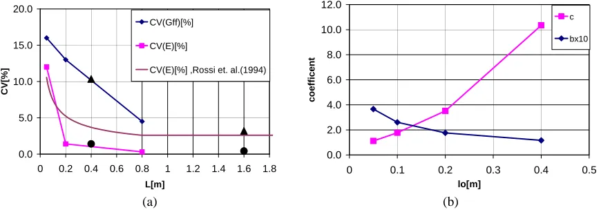
Figs. 3 (a) to (d) show the normalized effective stress-strain curves obtained by simulation for cubes samples varying from 0.20 to 1.60m. The expected curves are presented in Fig. 4(a) while Fig. 4 (b) shows normalized constitutive relations for axial elements with Lo varying in the range 0.05 and 0.40m. The graph clearly shows that the shape of the constitutive relations is affected by the size of the elements. The evolution of the CV of both E and Gf is shown in Fig. 5(a). The Figure also shows a plot of eq.(13) proposed by Rossi et al (1994) for the coefficient of variation of E, which is compatible with the results presented herein. Finally, Fig. 5(b) presents the dependence on the correlation length Lo of parameters b and c that characterize the behavior of axial elements. The preceding information underlines the basic result that not only the shape but also the parameters of the stress strain curve

change perceptibly with the size of the elements, fact the must be taken into consideration in the numerical analysis of non-linear structures.

0.0 5.0 10.0 15.0 20.0

0 0.2 0.4 0.6 0.8 1 1.2 1.4 1.6 1.8

L[m]

C

V

[%

]

CV(Gff)[%]

CV(E)[%]

CV(E)[%] ,Rossi et. al.(1994)

0.0 2.0 4.0 6.0 8.0 10.0 12.0

0 0.1 0.2 0.3 0.4 0.5

lo[m]

c

oe

ff

ic

e

nt

c

bx10

(a) (b)

Figure 5(a) Dependence of Young´s Modulus and Fracture Energy on cubic sample size and (b) Dependence of constitutive parameters b and c on axial elements length Lo.

The black triangles and dots in Fig 5(a) represent the CV of Gf and E obtained from the simulations with Lo.=0.10m and Lo.= 0.40m, i.e. for cubes with sides 0.40 and 1.60m, respectively, which are close to the values assumed in the analysis and serve as an indication of the correctness of those curves. Finally, it should also be pointed out that, as the size increases, the effective stress-strain or load-displacement curves tend to a linear diagram, with an abrupt, fragile rupture. If the element size is increased further, the diagram should have an unloading branch, after rupture, with a positive slope, to insure a correct value of the energy dissipated by fracture. Such a situation would not be admissible in a solution by numerical integration in the time domain, and leads to a maximum size of the DEM or FEM elements that may be used in a numerical model. In the present application of the DEM, for concrete structures, the maximum length Lo results slightly smaller than 0.50m.

CONCLUSIONS

It is shown that numerical predictions of the failure load of concrete structures, accounting for size effects, require the adoption of appropriate constitutive relations. These relations depend both on the size of the elements and on the correlation lengths of the random fields that describe the relevant material properties. In the paper a general expression for the stress-strain relation in tension is advanced, whose parameters can be related to standard properties of the material, such as Young´s modulus or its Specific Fracture Energy and to the size of the element. The simulations conducted for a typical concrete with largest aggregate size equal to 2.5cm led to constitutive curves for elements in the range between 0.20 and 1.60m. It may be seen that as size increases, the effective stress-strain diagram becomes increasingly linear, with a sudden rupture, while at the same time the CVs of the relevant parameters decrease to negligible values, situation that conditions the applicability of Linear Elastic Fracture Mechanics (LEFM). This is rarely the case in concrete structures, but may be common in Rock Mechanics.

ACKNOWLEDGEMENTS

The authors acknowledge the support of CNPq and CAPES (Brasil).

REFERENCES

1-Rios, R.D and Riera, J.D. (2004):. “Size effects in the analysis of reinforced concrete structures”, Engineering Structures, Elsevier, 26, 2004, 1115-1125.

2-Leonhart, F. and Walker, R. (1961): “The Stuttgart shear tests”, Translation No. 11, C&CA, London, . Beton und Stahlbetonbau, Vol. 65, no. 12, 1961, Vol. 57, No. 2, 3, 7 & 8.

3-Ramallo, J.C., Kotsovos, M.D. and Danesi, R.D.(1995), “Unintended out-of-plane actions in size

effects tests of structural concrete”, Transactions, 13th Int. Conf. on Structural Mech. In reactor Tech. (SMiRT 13), Vol. 3, 351,357.

4-Van Vliet M.R.A, Van Mier, J.G.M, “Size effects of concrete and sandstone”, HERON, Vol 45, No.2, 2000, 91-108.

5-Bazant , Z. P. (1976). "Instability, ductility, and size effect in strain-softening concrete", J.Eng. Mech. Div. 102, EM2, 331-344; disc 103, 357-358, 775-777, 104, 501-502.

6-Bazant, Z. P.(1993) "Scaling laws in the mechanics of failure", J. of Enineering Mecanics Div., Transactions, ASCE, Vol. 119, (9), pp. 1828-1844, 1993.

7-Weibull, W. ,"Statistical representation of fatigue failures in solids", Proceedings, Royal IT 27, 1949.

8-Rocha, M. M., and J. D. Riera (1990), On size effects and rupture of nonhomogeneous material. In: Van Mier JGM, Rots JG, Baker A, editors. Proceedings, Congress in Fracture Processes in Concrete, Rock and Ceramics. London: Chapmen & Hall/Ed. Fn. Spon, p.451-60.

9- Riera, J. D., and I. Iturrioz (1998), Discrete elements model for evaluating impact and impulsive response of reinforced concrete plates and shells subjected to impulsive loading, Nuclear Engineering and Design, 179, 135-144.

10-Wittman, F.H.; Roelfstra, H.; Mihashi,H.; Huang, y. T. and Zhang, X.H. (1987): Influence of age of loading, water-cement ratio and rate of loading on fracture energy of concrete, Materials and Structures, 20, 103-110. 11-Roelfstra, P.E. and Wittmann, F.H. (1987) Numerical modelling of fracture in concrete, Transactions, 9th

International Conf. on Structural Mechanics in Reactor Technology (SMiRT 9), Laussane, Switzerland, August 1987, Balkema, Rotterdam, Vol. H, 41-49.

12-Rossi, P. and Richer, R. (1987): “Numerical modeling of concrete cracking based on a stochastic approach”, Materials and Structures, 20, 334-337.

13-Rossi, P; Wu, X.; Le Maou, F. and Belloc, A. (1994): “Scale effects on concrete in tension”, Materials and Structures, 27, 437-444.

14-Rossi, P.; Ulm, F-J and Hachi, F. (1997): “Compressive behavior of concrete: physical mechanisms amd modeling”, ASCE J. of Engineering Mechanics, 122, 11, 1038-1043.

15-Fairbairn, E.M.R.; Paz, C.N.M.; Ebecken, N.F.F. and Ulm, F-J (1999), “Use of neural networks for fitting of FE probability scaling model parameters”, International Journal of Fracture, 95, 315-324.

16-Nayfeh, A. H., and M. S. Hefzy (1978), Continuum modeling of three-dimensional truss-like space structures, AIAA Journal, 16(8), 779-787.

17-Dalguer, L. A., K. Irikura, and J. D. Riera (2003), Simulation of tensile crack generation by three-dimensional dynamic shear rupture propagation during an earthquake, J. Geophys. Res., 108(B3), 2144, doi:10.1029/ 2001JB001738.

18-Riera J.D., Rocha M. M. ,"A Note on the Velocity of Crack Propagation in Tensile Fracture ", J. of the Braz. Soc. Mech. Sc. Vol XIII. N:3-pp217-240-1991.

19-Hillerborg, A. (1971): “A model for fracture analysis”, Cod. LUTVDG/TVBM 300-51-8.

20-Riera, J.D. and Iturrioz, I. (2005): “On the fracture analysis of concrete structures taking into consideration size effects”. Transactions, International Conference on Structural Mechanics in Reactor Technology, SMiRT 18, Beijing, China.

21-Morquio, A., and J. D. Riera (2004), Size and strain rate effects in steel structures, Engineering Structures, 26, 669-679.