A Compound Poisson Process for Relaxing the Molecular Clock

Copyright2000 by the Genetics Society of America

A Compound Poisson Process for Relaxing the Molecular Clock

John P. Huelsenbeck,* Bret Larget

†

_{and David Swofford}

‡

*Department of Biology, University of Rochester, Rochester, New York 14627,†_{Department of Mathematics and Computer Science,}

Duquesne University, Pittsburgh, Pennsylvania 15282 and‡_{Laboratory of Molecular Systematics,}

Smithsonian Museum Support Center, Suitland, Maryland 20746 Manuscript received March 22, 1999

Accepted for publication December 17, 1999

ABSTRACT

The molecular clock hypothesis remains an important conceptual and analytical tool in evolutionary biology despite the repeated observation that the clock hypothesis does not perfectly explain observed DNA sequence variation. We introduce a parametric model that relaxes the molecular clock by allowing rates to vary across lineages according to a compound Poisson process. Events of substitution rate change are placed onto a phylogenetic tree according to a Poisson process. When an event of substitution rate change occurs, the current rate of substitution is modified by a gamma-distributed random variable. Parameters of the model can be estimated using Bayesian inference. We use Markov chain Monte Carlo integration to evaluate the posterior probability distribution because the posterior probability involves high dimensional integrals and summations. Specifically, we use the Metropolis-Hastings-Green algorithm with 11 different move types to evaluate the posterior distribution. We demonstrate the method by analyzing a complete mtDNA sequence data set from 23 mammals. The model presented here has several potential advantages over other models that have been proposed to relax the clock because it is parametric and does not assume that rates change only at speciation events. This model should prove useful for estimating divergence times when substitution rates vary across lineages.

T

HE molecular clock hypothesis states that the evolu- substitution process. As an analytical tool, the molecular tionary rate of a gene is roughly constant among clock has also proven useful. Many of the more interest-different lineages (ZuckerkandlandPauling1962). ing applications of phylogenies assume that the

molecu-ZuckerkandlandPauling(1965) also suggested that lar clock holds. For example, statistical analysis of

host-the substitution process is approximately Poisson. If host-the parasite cospeciation often assumes a molecular clock rate of substitution is constant across lineages, then the (Huelsenbecket al. 1997). Also, the estimation of

diver-distances between species should be ultrametric (i.e., gence times using molecular data depends upon (1) an all tips are an equal distance from the root of the tree). accurate calibration date for at least one speciation Furthermore, if the substitutions follow a Poisson pro- event on the tree and (2) a constant substitution rate cess, then the variance and the mean of the number of _{among lineages. Several recent studies have attempted} substitutions that occur on different lineages in the _{to date the divergence times for eubacteria/eukaryotes} same amount of time should be equal. Since the early _{(Doolittle et al. 1996), metazoa (Wray et al. 1996),} 1970s, however, neither prediction has been shown to _{birds (Cooperand Penny1997), mammalian orders,} hold true; the variance to mean ratio of the number of _{and major lineages of vertebrates (KumarandHedges} substitutions is generally greater than one, suggesting _{1998) using the molecular clock assumption. To a large} that the substitution process is overdispersed (Ohta _{extent, the validity of any such analysis depends on how}

and Kimura 1971; Langley and Fitch 1973, 1974). _{well the data conform to the clock assumption.}

Moreover, rates of substitution have been shown to vary _{Several different approaches have been taken to}

ac-across lineages (seeGillespie1991). _{commodate rate variation among lineages. One}

Despite the observation that the molecular clock hy- _{method, commonly used for estimating phylogenetic} pothesis does not perfectly explain the substitution pro- _{trees, is to assign each branch of a phylogenetic tree its} cess, it remains a powerful conceptual and analytical _{own rate parameter. However, this procedure does not} tool in evolutionary biology. Conceptually, the molecu- _{allow estimation of divergence times of clades because} lar clock provides a timescale, albeit an imperfect one, _{rate and time are confounded. Another approach was} for evolution as well as a mechanistic description of the _{proposed by Sanderson(1997), who used a}

nonpara-metric method for smoothing the rate differences across speciation events on the tree. Sanderson’s method Corresponding author: John P. Huelsenbeck, Department of Biology,

allows rates to vary on branches of the tree and also University of Rochester, Rochester, NY 14627.

E-mail: [email protected] allows divergence times to be estimated. At the other

extreme,Thorneet al. (1998) proposed a parametric scaled branch lengths is referred to as the total length of the tree, T. The total length of the tree of Figure 1, model for relaxing the clock. LikeSanderson(1997),

they assume that rates are autocorrelated across specia- for example, is T⫽4.55. If the branch lengths are multi-plied by a parameter m, representing the expected num-tion events; their model assigns new rates to descendent

lineages from a lognormal distribution with the mean ber of substitutions per site on a single branch reaching from the root of the tree to the tips, the branch lengths of the distribution equal to the rate of the ancestral

lineage. The model we present here differs from the of the tree are in terms of expected number of substitu-tions per site. Moreover, the branch lengths on the models proposed bySanderson(1997) andThorneet

al. (1998) by allowing rates to change anywhere on tree conform to a molecular clock; there has been no variation in rates across lineages with the result that all the tree. Yet, the model introduces only two additional

parameters over the strict molecular clock. of the tips can be drawn to lie on a single time line. Figure 2 shows a rescaling of the tree of Figure 1 with In this article, we propose a compound Poisson

pro-cess for introducing rate variation across lineages on a m⫽0.17.

We use a compound Poisson process to introduce rate tree. We assume that nucleotide substitutions occur

along branches of the tree according to a Poisson pro- variation across lineages of the tree. Events (positions on the tree at which substitution rate changes) occur cess, as in the Markov substitution models widely used

for phylogenetic inference. However, an independent according to a Poisson process with parameter␭. When an event occurs, the rate of substitution just prior to the Poisson process also generates events of

substitution-rate change. At each of these events, the substitution-rate of substitu- event (m) is multiplied by a gamma-distributed random tion is changed by multiplying the current rate by a variable (taking value r) to produce a new substitution gamma-distributed random variable. We use Markov rate above the event (m⬘; m⬘ ⫽mr). The gamma

distribu-chain Monte Carlo when making Bayesian inferences. tion has density

⌫(r|␣,␤)⫽ ␤ ␣

C(␣)r

␣⫺1_e⫺␭r_{, r}ⱖ _{0, (1)}

METHODS

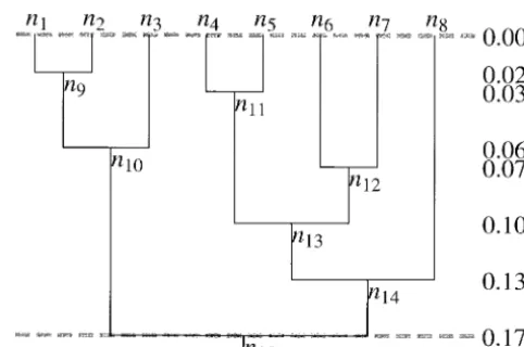
A compound Poisson process of rate variation: We _{where␣is the shape parameter and␤is the scale} param-assume that the phylogeny of a group of species can be _{eter. One possible parameterization of the gamma} distri-represented by a rooted binary tree, an arbitrary exam- _{bution that we initially considered is to set␣ ⫽ ␤ ⫽ ␣}

P,

ple of which is shown in Figure 1. The tips are labeled _{so that r is⌫(r|␣}

P,␣P). The mean rate of change, then,

n1to ns, and the internal nodes are labeled ns⫹1to n2s⫺1, _{is E[r]}⫽_{1. A potentially unappealing property of such}

where s is the number of sequences. The root of the _{a model of rate change is that as the branch lengthens,} tree is always labeled n2s⫺1. The times of the nodes are _{substitutions stop happening along the branch. In such}

denotedt⫽(t1, t2, . . . , t2s⫺1). The branches are scaled

such that the tips are at time 0 (t1⫽t2⫽. . .⫽ts⫽0)

and the root is at time 1 (t2s⫺1 ⫽ 1). The sum of the

Figure2.—The branch lengths that result when the tree of Figure 1 has all branches multiplied by m⫽0.17. The rate of substitution on the tree, m, is in terms of expected number of substitutions per site that occur along a single lineage reach-Figure1.—We assume that a rooted binary tree describes

the genealogy of the sequences n1to ns. This arbitrarily chosen ing from the root of the tree (t ⫽ 1) to the tips (t ⫽ 0).

Multiplying the branch lengths in Figure 1 by m converts tree illustrates the labeling of the nodes used in this article.

The unscaled times of the tree have the tips at time 0 and branch lengths into expected number of substitutions per site. Note that this tree has no rate variation among lineages. The the root at time 1. All other nodes on the tree have times

a model, the rate along a branch is a base rate, m, multiplied by ⌸n

iri, where n is the number of Poisson

change points and riis⌫(␣P,␣P). As the branch length

grows, n becomes large and the product converges to 0 in probability.

A prior model that changes rates multiplicatively with independent multipliers must be carefully chosen so that the rate does not tend to either 0 or infinity in probability. To see this, let ri, i⫽1, 2, . . . be independent

and identically distributed positive random variables and let Rn⫽ ⌸ni⫽1 ri. Then for everyε⬎0,

P[Rn⬍ε]⫽P

冤

兿

n

i⫽1

ri⬍ε

冥

Figure 3.—The compound Poisson process discussed in

⫽P

冤

兺

n

i⫽1

log Ri ⬍logε

冥

. this article places events of substitution-rate change on the

tree according to a Poisson process. Associated with each event is a rate multiplier that multiplies the rate of substitution up

Thus, the product of rates converges in probability to _{to the event (m) by a gamma-distributed random variable} 0 if E[log ri]⬍0 and increases without bound in proba- (taking value r) to produce a new rate of substitution above

the event (m⬘). In this example, which illustrates the process

bility if E[log ri]⬎ 0.

for the tree from Figure 1, three events of substitution-rate

In this article, we largely circumvent this problem by

change occur. The rate multipliers are 2.871, 1.103, and 0.776

placing a prior on␭ such that the number of change _{for events 1, 2, and 3, respectively. The z}

ispecify the event

points on the tree does not become large. In addition, _{locations on the tree.} we define a one-dimensional family of

gamma-distrib-uted random variables with the property that E[log ri]⫽

0 by letting␤ ⫽e␺(␣P)_{, where} ␺_{is the derivative of the}

[0,T] to points on the tree. Figure 3 illustrates the com-logarithm of the gamma function:

pound Poisson process for rate change events acting upon the tree of Figure 1. In this example, three events ␺(␣)⫽ d

d␣log C(␣) of rate change occur on the tree [e⫽(3,z,r),z⫽(1.354,

3.009, 4.301),r⫽(2.871, 1.103, 0.776)]. Associate each branch with the smaller number of its two nodes (that ⫽ C⬘(␣)

C(␣) node that is furthest from the root of the tree) and

partition the interval [0, T] into segments associated with branches ordered from the lowest index to the ⫽

共冮

∞

0(log x)x

␣⫺1_e⫺x_dx

兲

/

共冮

0∞x

␣⫺1_e⫺x_dx

兲

_.

highest index. For example, the branch descending from node n1is represented by the interval [0, 0.125].

Here is a short derivation of this property. Suppose that

Similarly, the branch descending from node n6is

repre-rⵑ⌫(␣,␤). Then r is equal in distribution to X/␤where

sented by the interval (0.979, 1.416]. The first event is

Xⵑ⌫(␣,1):

located on this branch at z1 ⫽ 1.354. Events 1 and 2

E[log r]⫽E[log(X/␤)] increase the rate of substitution whereas event 3 de-creases the rate of substitution. Figure 4 shows the rela-⫽

冮

∞

0(log x)

1 ⌫(␣)x

␣⫺1_e⫺x_dx⫺ _log␤

tive branch lengths in terms of expected number of substitutions per site. Note that the branch lengths of the tree no longer obey the molecular clock. The molec-⫽ ␺(␣)⫺ log␤.

ular clock is simply a special case of our model with␭ ⫽ This is 0 precisely when␤ ⫽ e␺(␣)_.

0 and/or␣P⫽∞.

In this article, we multiply the rate at an event by a _{The prior distribution of e⫽(␰,z,r) given the tree} gamma-distributed random variable with density _{and parameters␣Pand␭is described by the probability}

measure

g(r|␣P)⫽

e␺(␣P)

⌫(␣P)

r␣P⫺1_e⫺re␺(␣P)_{, r}ⱖ_{0. (2)}

f(e|␶, t,␭,␣P)⫽e⫺␭T␦0⫹

兺

∞

␰⫽1

e⫺␭T_{(␭T )}␰

␰! ⫻

冢

1 T冣␰

⫻

_兺

␰

i⫽1

g(ri|␣P),

The collection of events is denotede⫽(␰,z,r), where

(3) ␰is the number of rate change events, z is the vector

of event positions, andris the vector of rate multipliers. where ␦0 is the point mass measure at (0, 0/, 0/). This

When␰ ⫽0,z andrare empty. For␰ ⬎ 0,z苸 [0,T]␰ corresponds to picking a Poisson (␭T ) number of

HKY85 model of DNA substitution (Hasegawa et al.

1984, 1985). This model allows different base frequen-cies and for a transition/transversion rate bias (rAG ⫽

rCT; rAC ⫽ rAT⫽ rCG ⫽ rGT; ␬ ⫽ rAG/rAC). The transition

probabilities are calculated asP(v)⫽{pij(v)}⫽ eQv.

Among-site rate variation can be accommodated in several different ways. One potential method partitions the DNA sequence into different regions (e.g., first, sec-ond, and third codon positions) and then estimates the rate separately for each partition, assuming that the rate within a partition is homogeneous [i.e., instead of a single substitution rate (m), applying to all sites, there are multiple substitution rates (m1, m2, . . . )]. Another

method assumes that the rate assigned to a site is a random variable. Typically, the gamma distribution, pa-rameterized with the shape parameter equal to the scale parameter, is used to model rate variation across sites (Yang1993, 1994a). The shape parameter of the gamma distribution for among-site rate variation is denoted␣R.

Figure4.—The branch lengths in terms of expected

num-ber of substitutions per site when the substitution rates are In this article, we assume equal rates across sites or

modified using the compound Poisson process. The rates were _{gamma-distributed rates across sites. Models that assume} modified using the three events from Figure 3 with a starting _{gamma-distribution rate variation are denoted “⫹⌫.”} substitution rate of m⫽0.17 (at the root of the tree). Note

Our implementation of gamma-distributed rate

varia-that the branch lengths of the tree no longer conform to the

tion uses the discrete gamma approximation with four

molecular clock.

rate categories (Yang1994a).

The probability of observing the states present at the

ith site (xi) is a sum over all possible assignments of

dent uniform [0,T] distributions, and attaching mutu- _{nucleotides to the internal nodes of the tree. Suppose} ally independent gamma-distributed rate multipliers. _{y ⫽ {yk} for k ⫽ s ⫹ 1, . . . , 2s ⫺ 1 is a generic data}

Model of DNA substitution: We assume that DNA _{vector at the internal nodes. Branch k of the tree has} sequences from homologous regions are available for _{length vkexpected substitutions per site and ancestral} species n1to ns. LetX⫽{xij} be the aligned nucleotide node ␴(k). The transition probability from state i to

sequences, where i⫽1, 2, . . . , s ; j⫽ 1, 2, . . . ,c ; and _{state j along a branch with v expected substitutions is}

c is the number of nucleotide sites per sequence. Each _{pij(v). The initial substitution rate at the root is m. Then,}

column of the data matrix xj ⫽ {x1j, . . . , xsj}⬘specifies the conditional probability of observing the data at the

the nucleotides for the s sequences at the jth site. _{ith site given the tree and rate events is} As is usual for DNA sequences, we assume that

substi-tutions occur according to a Poisson process with rate _f(xi|␶,t,e, m)⫽

兺

y

␲y2s⫺1

冢

兿

s

k⫽1

py_␴(k)xk(vk)

冣 冢

兿

2s⫺2

k⫽s⫹1

py_␴(k)yk(vk)

冣

.

matrixQ. A general reversible rate matrix allows a

differ-ent stationary frequency for the four nucleotides␲ ⫽ ₍₅₎

(␲A,␲C,␲G,␲T) constrained to sum to one and six rates

The summation is over all possible combinations of for the 12 substitution types

nucleotide states that can be assigned to the internal nodes of the tree. The expected number of substitutions on branch k (vk) is found by integrating the rate over

Q⫽ {qij}⫽









. ␲CrAC ␲GrAG ␲TrAT

␲ArAC . ␲GrCG ␲TrCT

␲CrAG ␲CrCG . ␲TrGT

␲ArAT ␲CrCT ␲GrGT .









(4) _{the length of the branch, v}

k⫽兰tkt_␴(k)rk(u)du, where rk(u)

is the rate along branch k at time u. The rate is a step function for the compound Poisson process considered (Yang1994b). The diagonal of the rate matrix is

speci-in this article. Figure 5 shows a sspeci-ingle branch startspeci-ing fied such that the row sums are equal to zero. We add

at tB ⫽ 0.40 and ending at tE ⫽ 0.20. There are two

an additional constraint by rescaling so that⫺Rqii␲i ⫽

events of substitution-rate change along this branch, 1; this means that branch lengths of the tree are in

occurring at times 0.30 and 0.25. The expected number terms of expected number of substitutions per site, v.

of substitutions per site along this branch, then, is This model is reversible because it fulfills the

reversibil-ity criterion that␲iqij ⫽ ␲jqji for all i and j. Most com- v⫽(0.40⫺0.30)⫻0.10⫹ (0.30⫺ 0.25)

monly used models of DNA substitution are constrained _⫻

0.12⫹(0.25⫺0.20)⫻0.06 to be reversible and are simply special cases of the model

a joint prior probability distribution for the parameters ␭, ␣P, and m along with the rate events and branch

lengths.

All Bayesian inference arises from the joint posterior distribution of the parameters of interest (in this case, the posterior distribution of␭,␣P, and m). The posterior

probability density of␭,␣P, and m is

f(␭,␣P, m|X)⫽

ᐉ(␭,␣P, m)f(␭,␣P, m)

f(X) , (9)

where

f(X)⫽

冮

_␩ᐉ(␭,␣P, m)dF(␭,␣P, m)

and␩is the space for␭,␣P, and m. We assume that␭,

␣P, and m have independent priors. The parameters␣P

and m have uniform priors on [0, B␣P] and [0, Bm],

respectively. We place an exponential prior on␭. The

Figure 5.—An example of how the average number of

relative speciation times,t, which are scaled to be

be-substitutions per site is calculated for a branch when

substitu-tion rate changes through time. Here, the substitusubstitu-tion rate _{tween 0 and 1 (see Figure 1), are distributed as the} changes according to the compound Poisson process used in _{order statistics drawn from a uniform (0, 1) distribution,} this article. There are two events of substitution rate change

conditional on agreement with the tree topology ␶.

along this branch. The first doubles the current substitution

There is no biological meaning to the uniformly

distrib-rate and the second halves the current substitution distrib-rate.

uted priors. However, in Bayesian analysis, such priors are often used in cases where there is little or no prior knowledge about the parameters. Using uninformative The substitution rate at the base of the branch is m⫽ _{priors is a way to avoid biasing the results of the analysis;}

0.10. _{the posterior probability distribution will mainly be}

de-Assuming independence of the substitutions across _{termined by the likelihood function. An exponential} sites, the conditional probability of observing the full _{prior on␭decreases the probability of substitution rate} sequence data set given the tree and rate events is the _{histories with a large number of small rate-change events.} product of the probabilities of observing the sites: _{Calculation of the posterior probability density} (Equa-tion 8) involves evaluating high-dimensional integrals

f(X|␶,t,e, m)⫽

兿

c

i⫽1

f(xi|␶,t,e, m). (7) _{and summations. We use Markov chain Monte Carlo}

(MCMC) integration to estimate the posterior

distribu-Estimating m, ␭, and ␣P using Markov chain Monte _{tions of interest. Specifically, we used the} Metropolis-Carlo:We wish to estimate the rate of molecular evolu- _{Hastings-Green (MHG) algorithm (Green 1995; see} tion at each branch through Bayesian estimation of the _{alsoGeyer1999), an extension of the} Metropolis-Has-parameters␭,␣P, and m (where m is the rate of substitu- _{tings algorithm for problems in which the dimension}

tion at the base of the tree). The likelihood function _{of the sample space changes. The MHG algorithm}

con-for␭,␣P, and m is _{structs a Markov chain by first proposing a new state}

and then moving to that state with probability R. The

ᐉ(␭,␣P, m)⫽

冮ε

f(X|␶,t,e, m)dF(e|␶, t,␭,␣P)dF(t),

steps of the algorithm are as follows: (1) the current state of the chain is␪; (2)with probability density f(␪*|␪), (8)

a new state (␪*) is nominated; (3) the acceptance proba-where the single integral denotes integration over all

bility of the nominated state is calculated, rate events and branch lengths consistent with the tree

topology␶. Integration with respect to the probability

R⫽min

冦

1,f(␪*)f(␪|␪*)

f(␪)f(␪*|␪)

冧

, (10) measure is used to denote a summation for discrete

random variables (such as the number of events on a

where f(␪) is the target distribution (i.e., Equations 7 tree or the topology of a tree) as well as integration for

or 8); and (4) a uniformly distributed random variable continuous random variables (such as the position of

on the interval [0, 1] is generated. If this random vari-the events, vari-the speciation times, and vari-the

gamma-distrib-able is ⬍R, then the nominated state is accepted and

uted rates associated with events). The tree topology is

becomes the current state of the chain (␪ ⫽ ␪*). Other-considered to be fixed in this study, but the speciation

wise, the chain remains in state␪. Steps 1–4 are repeated times and the position and rates of events are treated

Several different mechanisms were used to update tree. The first move type (3a) was chosen with probabil-ityφ3aand picked at random one of the␰events on the

the state of the chain. These mechanisms included (1)

adding an event to the tree, (2) deleting an event from tree. A new position was chosen uniformly on the interval [0, T]. The second move type (3b) was chosen with proba-the tree, (3) changing proba-the position of an event on proba-the

tree, (4) changing the gamma-distributed random vari- bility φ3band picked one of the␰ events on the tree at

random and moved its current position by a small able associated with an event on the tree, (5) changing

the time of an internal node on the tree, (6) changing amount randomly drawn from the interval [⫺ε3b,⫹ε3b].

The acceptance probability for both of these moves is the substitution rate (m) at the base of the tree, (7)

changing the Poisson parameter (␭), (8) changing the

R⫽ min{1, (likelihood ratio)}. (15) gamma parameter (␣P), (9) changing the transition/

transversion rate ratio (␬), (10) changing the gamma Move type 4: Changing the rate multiplier associated with

shape parameter for among-site rate variation (␣R), and an event: Two different move types changed the rate

(11) changing the base frequencies (␲). associated with an event on the tree. Both move types The acceptance probabilities for the different moves pick at random one of the ␰ events. This randomly

take the form chosen event will have its rate multiplier changed from

r to r *. For the first move type (4a) a change to r * is R⫽min{1, likelihood ratio)⫻(prior ratio)

proposed with probability φ4a such that loge(r */r) is ⫻(proposal ratio)⫻ ( Jacobian)} (11) uniformly distributed on the interval [⫺1_⁄

2, ⫹1⁄2]. The

acceptance probability for this move is then

(Green1995). For move types 3–8, the standard Markov

chain theory employed in the Metropolis-Hastings algo- R⫽min{1, (likelihood ratio) ⫻(r */r)␣P_e⫺(r*⫺r)e␺(␣P)

} rithm (Metropoliset al. 1953;Hastings1970) applies.

(16) However, move types 1 and 2 add and delete an event,

respectively. These move types involve a change in the (Green1995). The other move type (4b) is chosen with dimensionality of the sample space. Hence, we construct _{probabilityφ4band picks a new rate by drawing a random} reversible Markov chains for move types 1 and 2 that jump _{variable from the distribution g(r*|␣P). The acceptance} between parameter subspaces of different dimensional- _{probability for this move type is simply the likelihood} ity using the methodology developed byGreen(1995). _{ratio (Equation 15).}

Move type 1: Adding an event to the tree: The prior ratio _{Move type 5: Changing the time of an internal node on the}

for the addition of a single point (z*, r *) to the current _{tree: With probability φ5, the time of an internal node}

state e⫽(␰,z,r) is _{was changed. The times of the internal nodes were}

up-dated as follows. First, an internal node of the tree was

[(e⫺␭T(␭T )␰⫹1/(␰ ⫹_1)!)⫻_{(1/T )}␰⫹1⫻

兿

␰

i⫽1g(ri|␣P)

chosen at random (excluding the root node). The time of this node was increased or decreased by adding a

⫻g(r *|␣P)]/[(e⫺␭T(␭T )␰/␰!)⫻(1/T )␰⫻

兿

␰i⫽1g(ri|␣P)]

uniformly distributed random variable drawn from the

⫽ ␭g(r*|␣P)/(␰ ⫹1) (12) _{interval [}⫺ε

5,⫹ε5]. The acceptance probability for this

move is and the proposal ratio is

R⫽min

冦

1, (likelihood ratio)⫻ e

⫺␭T*₍␭_T*)␰

e⫺␭t₍␭_T)␰ ⫻

T T*

冧

, d␰⫹1⫻1/(␰ ⫹1)

b␰⫻1/(␰ ⫹1) ⫻1/T⫻g(r *|␣P)

⫽ Td␰⫹1

g(r *|␣P)b␰

,

(17) (13)

where T* is the total tree length after the node time where d␰⫹1and b␰are the probabilities of making a move _{has been adjusted. A change to the speciation time on}

that deletes one of␰ ⫹1 events or adds an event when _{an internal node affects the length of a total of three} there are currently␰events, respectively. The Jacobian _{branches (the ancestral branch and the two descendant}

is 1. The acceptance probability, then, is _{branches). Often, events of rate change occur along}

these branches. The times of the rate-change events are

R⫽min

冦

1, (likelihood ratio)⫻ ␭Td␰⫹1

(␰ ⫹1)b␰

冧

. (14) maintained proportionally along the same branch they started on.

Move types 6, 7, 8, 9, and 10: Changing m,␭,␣P,␬, and

Move type 2: Deleting an event from the tree: The

accep-tance probability for the reverse step, deleting an event ␣R: The substitution rate (m), Poisson parameter (␭),

gamma shape parameter (␣P), transition/transversion

from the tree, has the same form as Equation 13, but

with the ratio terms inverted. Detailed balance between rate ratio (␬), and gamma shape parameter for among-site rate variation (␣R) were updated with probabilities

the move types that add and delete an event on the tree

is demonstrated in theappendix. φ6,φ7,φ8,φ9, andφ10, respectively, by adding to the

cur-rent value a uniformly distributed random variable on

Move type 3: Changing the position of an event: Two

⫹ε9], and [⫺ε10, ⫹ε10], respectively. The acceptance

probabilities are _␪

*⫽

冦

l⫹(l ⫺ ␪⬘):␪⬘ ⬍l

␪⬘:lⱕ ␪⬘ ⱕh

h⫺ (␪⬘ ⫺h):␪⬘ ⬎h.

(23)

R⫽ min{1, (likelihood ratio)} (18)

for the update of m,␬, and␣R, _{The proposal ratio [in (10)] is one for this type of}

proposal.

R⫽min

冦

1, (likelihood ratio) ⫻e

⫺␭*T₍␭_*T)␰

e⫺␭T(␭T)␰

冧

(19) _{was sampled every g}Estimating parameters using Bayesian inference: The chain

Sgenerations. The posterior

distribu-tions of the parameters are obtained directly by noting for the update of␭, where␭* is the proposed state and

the position of the chain and recording the values of ␭is the current state, and

m,␭, and ␣P for each sampled state. The proportion

of the time the chain stays in different intervals is an

R⫽min

冦

1, (likelihood ratio)⫻

兿

␰

i⫽1

g(ri|␣*P)/g(ri|␣P)

冧

(20)

approximation of the posterior distribution.

The chain was burned in by discarding the first gB

for the update of␣p, where␣*P is the proposed state and _{generations of the Markov chain. The burn-in was} per-␣Pis the current state. We also considered gamma priors

formed to allow the chain to approach stationarity be-for m, ␭, and ␣P. The gamma prior has parameters a

fore states are sampled. and b. The exponential prior for␭used in the analyses

Validation of computer program: A computer pro-of this article has a⫽ 1. A change to m* is proposed

gram implementing the compound Poisson process for such that loge(m*/m) is uniformly distributed on the

the HKY85 ⫹ ⌫ (Hasegawa et al. 1984, 1985; Yang

interval [⫺1_⁄

2,⫹1⁄2]. The acceptance probability for this

1993, 1994a) model of DNA substitution was written in move is then

C by one of us ( J.P.H.; available via anonymous ftp to brahms.biology.rochester.edu or via the WWW at http://

R⫽min{1, (likelihood ratio)⫻ (m*/m)a_e⫺b(m*⫺m)_}.

brahms.biology.rochester.edu). The advantage of using (21)

MCMC for Bayesian inference is that the sampled points The acceptance probabilities for changing␭and␣pare are a valid (albeit dependent) sample from the posterior

the same as Equation 21, with m and m* replaced by␭ _{distribution: the Markov chain law of large numbers} and␭* and␣pand␣*p, respectively. (theorem 3;Tierney1994) states that posterior

proba-Move type 11: Changing the base frequencies: With proba- _{bilities can be validly estimated from long-run sample}

bilityφ11a move was attempted that changed the equilib- _{frequencies. However, it is impossible to guarantee that}

rium base frequencies,␲. The sum of the base frequen- _{an implementation of MCMC will converge for any} par-cies is constrained to equal 1 and new values are _{ticular problem (Geyer1999). AsGeyer(1999, p. 80)} proposed from a Dirichlet distribution with expected _{states, “MCMC is a complex mixture of computer} pro-values at the current pro-values. The Dirichlet distribution _{gramming, statistical theory, and practical experience.} is the natural conjugate prior for a multinomial distribu- _{When it works, it does things that cannot be done any}

tion and has probability density _{other way, but it is good to remember that it is not}

foolproof.”

f(␲|␣)⫽ ⌫(␣0) ⌸i苸S⌫(␣i)

兿

i苸S

␲(␣i⫺1)

i , (22) The computer program was validated in several ways:

(1) likelihoods were checked against existing computer programs (e.g., PAUP*;Swofford1998); (2) the accep-where S is the state space (A, C, G, or T), ␣i is the

tance probabilities for the various move types were Dirichlet parameter of the ith nucleotide,␣0 ⫽Riε苸S␣i,

worked out independently by two of us; and (3) the and␲iis the frequency of the ith nucleotide. New base

program was run without any data. When the program frequencies are drawn from the Dirichlet distribution

is run without any data, then the likelihood ratio equals with␣i⫽ ␲i␣0. We set␣0⫽100.0 in all of the analyses

one and the chain should target the prior distribution. of this study.

When the chain is run without data, the expectation

Changing parameters near the boundary of the parameter

and variance of the number of events on the tree should

space: Note that for move types 3b, 5, 6, 7, 8, 9, and 10

both be equal to␭T. Moreover, the average rate

associ-that the parameter is changed by adding a uniformly

ated with the events should equal␣P/e␺(␣P)and the

vari-distributed random variable from an interval [⫺ε,⫹ε].

ance should equal␣P/e␺(␣P). When the chain was run

When the parameter is restricted to an interval (l, h)

without data, the results satisfied these expectations. and the proposed value is outside this interval, we reflect

Also, multiple independent chains were started from the excess back into the interval. Namely, if␪⬘ ⫽ ␪ ⫹

different starting values of the parameters. The chains

U, where␪ is the current parameter value (either z, t,

were examined to see if they converged to the same

m,␭, or␣P) and U is the uniformly distributed change,

Analysis of DNA sequence data: We applied the ter values of the prior were used [m⫽0.33 (0.32, 0.33); method to a single DNA sequence data set. The data ␣P⫽63.89 (30.00, 104.24)]. The posterior distribution

set included complete mitochondrial sequences from of m became broader and the posterior distribution of␣P

23 mammals (Arnasonet al. 1997). The tree topology increased (there were more events, each with a smaller was considered fixed in the analysis; the tree topology effect). However, the branch lengths were very similar estimated using UPGMA (SokalandMichener1958) regardless of the exact value of the exponential prior with the Jukes-Cantor distance (Jukes and Cantor on ␭. Figure 10 shows the relationship between the 1969) was used in the analysis. All analyses were per- maximum-likelihood estimates of the branch lengths formed assuming the HKY85 model of DNA substitution obtained assuming the HKY85 model of DNA

substitu-(Hasegawaet al. 1984, 1985). This model allows differ- tion and the mean of the posterior distribution of each

ent base frequencies as well as a transition/transversion branch obtained under the compound Poisson process. rate bias. Parameters of the substitution model were In both cases, the compound Poisson process was able estimated on the UPGMA tree using maximum likeli- to accommodate rate variation across lineages of the hood (as implemented in PAUP*;Swofford1998). tree (the slope was 1.00, with r2⫽_{0.999 for both priors).}

The Markov chain was run for at least 500,000 genera- We also examined the relationship between the com-tions. Every 50th state of the chain was sampled (i.e., pound Poisson process with exponential priors of means

gS⫽50). The sampled states were used to construct the 1 and 10 (Figure 11). Again, there is a close relationship

posterior distribution for the variables m,␭, and␣p. between the branch lengths regardless of the prior used

for␭. The posterior distributions of branch lengths are quite robust to the two different priors used for␭.

RESULTS

The compound Poisson process for relaxing the mo-The molecular clock hypothesis of equal rates across _{lecular clock should prove practically useful for several} lineages could be rejected for the mammalian mtDNA _{applications. For example, estimation of divergence} sequence data set. We used a likelihood-ratio test to _{times for clades depends upon a calibration time for at} examine the molecular clock hypothesis (Felsenstein _{least one speciation event on the tree and equal rates}

1981). The HKY85⫹ ⌫model was assumed in the analy- _{across lineages (though seeSanderson1997). The} com-sis. The null hypothesis is that the molecular clock holds; _{pound Poisson process can be used to relax the} molecu-the likelihood is maximized under molecu-the constraint of _{lar clock while at the same time allow estimation of} equal rates across lineages (L0). The alternative hypothe- _{divergence times of clades. An application of the}

sis relaxes the clock constraint by assigning a different _{method applied to the mammalian mitochondrial data} rate to each of the lineages; the likelihood under the _{is shown in Figure 12. The general approach is the same} alternative hypothesis is L1. The likelihood-ratio test _{as that taken by Thorne et al. (1998), but we used}

statistic (twice the difference in the logelikelihood,⫺2 _{the compound Poisson process discussed in this article}

loge⌳;⌳ ⫽L0/L1) between the null and alternative mod- _{instead of a lognormal distribution to relax the clock}

els is approximately␹2_{distributed with s}⫺_{2 degrees of}

assumption. The estimation of divergence times re-freedom. The molecular clock hypothesis was rejected _{quired only one modification to the notation described} at the 5% level (mammalian mitochondrial sequences:

logeL0⫽ ⫺114,514.23, logeL1⫽ ⫺114,431.21,⫺2 loge⌳ ⫽

166.03, P⬍0.00001).

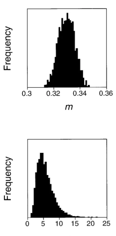
We assumed two different priors for␭for the mtDNA data. Figures 6 and 7 show the results of the analysis of the mammalian mitochondrial sequences assuming an exponential prior for␭ with mean 1.0. Figure 6 shows the change in the loge likelihood through time. The

probability of observing the data increased for the first 10,000 generations of the chain. The logelikelihood then

stabilized, fluctuating around a value ofⵑ⫺130,240. We discarded the first gB⫽50,000 generations as the

burn-in time of the chaburn-in. Figure 7 shows the posterior distri-butions for the parameters m and␣P. The estimates were

m⫽0.33 (0.32, 0.34) and␣P⫽5.70 (2.35, 10.82). The

credibility interval for each variable was determined by taking the 2.5% tails of the posterior distributions.

Figures 8 and 9 show the results of analyses in which

Figure6.—The change in the logeprobability of observing

an exponential prior with mean 10.0 was assumed for␭. _{the data (Equation 6) for the analysis of the mammalian} mito-Estimates of␣P(the shape parameter of the compound _{chondrial sequences. The prior for} ␭ _{was exponential with}

mean 1.

parame-in this article; parame-instead of rescalparame-ing branch times between date of 60 million years for the cow-whale divergence. We used a calibration date of 56.5 million years for 0 (at the tips) and 1 (at the root), the tips of the tree

the cow-whale divergence that is based on the earliest were considered to be time 0 and the times of other

occurrence of either artiodactyls or cetaceans. The esti-branches on the tree were in terms of millions of years

mate of the Ferungulate-Xenartha divergence is 92.5 before present. The HKY85⫹ ⌫model of DNA

substitu-mya (83.7, 99.6). The credibility interval overlaps the tion was assumed in the analysis; the gamma model fit

estimate obtained byArnason et al. (1997). In Figure

the observed sequences better than a model that pooled

12, we also indicate the divergence time estimates of sites according to codon position and allowed a different

the other clades on the tree, with the 95% credibility rate for each partition (logeL ⫽ ⫺114,431.21 for

intervals. HKY85⫹ ⌫, logeL⫽ ⫺117,091.83 for HKY85⫹SS). An

Two different priors were used in the analysis of the exponential prior with mean 0.006 was placed on ␭.

speciation times for the mammals. We used exponential The estimates of the substitution model parameters

priors with means 0.06 and 0.006 per million years. were m⫽0.010 (0.008, 0.012),␣P⫽7.58 (2.60, 17.13),

These numbers were chosen so that the means of the ␬ ⫽13.67 (13.00, 14.37), and␣R⫽0.230 (0.228, 0.240).

exponential priors were similar to the priors used earlier The posterior distribution of the divergence time of

(0.06⫻ 150 mya⫽ 10; 0.006 ⫻ 150 ⫽ 1). Figure 13 ferungulates (carnivores, perissodactyls, artiodactyls,

shows the relationship between estimates of speciation and cetaceans) and Xenartha (Edentata) is shown in

times for two different priors on ␭ for the mammal Figure 12.Arnasonet al. (1997) obtained an estimate

mtDNA data. We used exponential priors with means of 86 mya for this speciation event using a calibration

0.06 (x) and 0.006 (y). The x-axis shows that speciation times differed by at most 0.2 for the two priors. The estimates of speciation times appear robust to the choice of prior used for␭.

DISCUSSION

The molecular clock hypothesis, although useful in evolutionary biology, is inaccurate in two important de-tails; rates across lineages appear to vary and the substi-tution process deviates significantly from a Poisson pro-cess (Ohta and Kimura 1971; Langley and Fitch

1973, 1974; also seeGillespie1991). This article consid-ers only lineage effects on rate variation; that is, we only consider changes in the overall substitution rate that occur along different lineages through processes such as a change in the generation time. We do not relax

Figure8.—The change in the logeprobability of observing

the data (Equation 6) for the analysis of the mammalian mito-Figure7.—The posterior probability distributions for the

parameters m and␣Pfor the mammalian mitochondrial se- chondrial sequences. The prior for ␭ was exponential with

Figure9.—The posterior probability distributions for the parameters m and ␣P for the mammalian mitochondrial

se-quences. The prior for␭was exponential with mean 10.

Figure 10.—The Bayesian and maximum-likelihood esti-mates of the branch lengths for the mammalian mitochondrial

the assumption that the substitutions on a tree follow _{sequences are highly correlated (slope⫽ 1.0; r}2_{⫽ 0.999).}

a Poisson process. It is important to relax the assumption Bayesian estimates of branch lengths were taken as the mean of the posterior distribution. Both sets of branch lengths were

that rates are constant across lineages because almost

obtained under the HKY85 model of DNA substitution.

any study of the rate of substitution in DNA or amino acid sequences rejects the null hypothesis that rates across lineages are equal through time (Langleyand

Fitch1974;Goodmanet al. 1975;WuandLi1985). This of substitution for each lineage on a phylogenetic tree

is especially true now that biologists are using recently does not allow estimation of divergence times or allow available software that allows easy testing of the molecu- comparison of speciation times for different taxonomic lar clock hypothesis (e.g., PAML, Yang 1997; PAUP*, groups.Sanderson(1997) made an important advance

Swofford1998). in the estimation of divergence times using molecular

Several approaches have been taken to relax the mo- data by (1) showing how all of the sequences of a study lecular clock. The most frequently used method for can be used simultaneously to estimate the divergence relaxing the rate-constancy assumption is to assign a time of a clade and (2) relaxing the molecular clock by fixed rate parameter to each branch of a phylogeny. smoothing the rate differences across speciation times This solution works well for the phylogeny problem on a tree. Similarly,Thorne et al. (1998) relaxed the

cally plausible mechanisms that could cause rates to change in a nearly step-like manner. For example, any process that rapidly changes the substitution rate (such as a change in the proofreading mechanisms, a change in selective constraints, or a rapid change in the genera-tion time) can be approximately described using a step function. One of the main advantages of treating rate variation as a compound Poisson process is that the model can introduce rate variation across lineages at any point on the phylogenetic tree; other methods that have been considered assume that substitution rate changes at speciation events (e.g., Sanderson 1997;

Thorneet al. 1998). Such models may be sensitive to

taxon sampling. On the other hand, these solutions may prove to be more practical for data analysis because there are fewer parameters to estimate. The gamma distribution used to modify ancestral rates, however, is

Figure11.—The Bayesian estimates of branch lengths for _{not so easily justified using as an argument biological} the two exponential priors examined (1 and 10). The branch _{plausibility. We chose to use a gamma distribution to} lengths are highly correlated (slope⫽1.00; r2⫽_0.999).

Baye-modify rates because of its analytical tractability and

sian estimates of branch lengths were taken as the mean of

flexibility. Other methods for modifying rates, however,

the posterior distribution. Both sets of branch lengths were

obtained under the HKY85 model of DNA substitution. may work just as well.

We uncovered significant rate variation across lin-eages for the mammalian mitochondrial DNA sequence data sets. The clock hypothesis could be rejected using tion. They evaluated the posterior distribution of

specia-a likelihood-rspecia-atio test (Felsenstein1981). Importantly, tion times using MCMC.

the posterior distribution of the gamma parameter (␣P)

The compound Poisson process considered here

was close to 0, which also suggests that the data were models rate variation across lineages on a tree as a step

not consistent with the clock hypothesis. function. There were several reasons we chose to model

Other models may also prove useful for relaxing the rate variation as a step function, with a major reason

being analytical tractability. However, there are biologi- molecular clock assumption. For example, a doubly

to construct a more realistic probability distribution de-scribing the divergence time of a clade.

One important result of this article is that we demon-strate that events can be placed onto a phylogenetic tree under a Poisson process and estimation performed using MCMC. The Poisson process is one of the most useful models in biology, and there are several possible extensions of the approach we describe in phylogenet-ics. For example, one could place events onto a tree according to a Poisson process with each event changing the synonymous/nonsynonymous rate ratio, the base frequencies, or whether the site has a positive rate or a rate of zero (i.e., the covarion model). The advantage of this approach is that it allows the rate of nucleotide substitution to change on a tree under a biologically reasonable model with the addition of a small number of parameters.

This article benefited from discussions with Rasmus Nielsen and Michael Newton. Mary Kuhner provided suggestions for checking the results of the computer program. The suggestions of two anonymous reviewers also improved this article. J.P.H. and B.L. thank the Isaac Figure13.—The estimates of speciation times were similar Newton Institute for Mathematical Sciences and the National Science regardless of the exponential prior placed on␭. Two exponen- Foundation (NSF grant DMS-9804739) for their support in Cambridge tial priors with means 0.06 and 0.006 were examined. The during the summer of 1998. B.L.’s research was supported by NSF x-axis shows the proportion difference between the two esti- grant DBI-9723799.

mates of speciation time. x and y represent the speciation times for the exponential priors with means 0.06 and 0.006, respectively.

LITERATURE CITED

chastic (or Cox) process can be used to allow rates to

Arnason, U., A. GullbergandA. Janke,1997 Phylogenetic analyses vary through time (Gillespie 1991). In this process,

of mitochondrial DNA suggest a sister group relationship between the rate of substitution is drawn from some stationary _{Xenartha (Edentata) and Ferungulates. Mol. Biol. Evol. 14: 762–}

768. distribution r (u) (the rate at time u) with the transition

Cooper, A.,andD. Penny,1997 Mass survival of birds across the probabilities calculated as they were in this article.

Im-Cretaceous-Tertiary boundary: molecular evidence. Science 275: portantly, this process has a variance to mean ratio (in- _1109–1113.

dex of dispersion) greater than one. One of the main Doolittle, F. F., D.-F. Feng, S. Tsar, G. ChoandE. Little,1996 Determining divergence times of the major kingdoms of living difficulties of this process is the choice of the rate

distri-organisms with a protein clock. Science 271: 470–477. bution. It is not clear what distribution would be most _{Felsenstein, J.,1981 Evolutionary trees from DNA sequences: a} appropriate for modeling rate variation through time. maximum likelihood approach. J. Mol. Evol. 17: 368–376.

Geyer, C. J.,1999 Likelihood inference for spatial point processes, Also, if the rate distribution has too many parameters,

pp. 79–140 in Stochastic Geometry: Likelihood and Computation, ed-it may be difficult to estimate the parameters of the rate _{ited byO. E. Barndorff-Nielsen, W. S. KendallandM. N. M.} distribution while simultaneously allowing estimation of van Lieshout.Chapman and Hall/CRC, London.

Gillespie, J. H.,1991 The Causes of Molecular Evolution. Oxford Uni-other interesting parameters (such as the divergence

versity Press, Oxford.

time of a clade). _{Goodman, M., G. W. Mooreand G. Matsuda, 1975 Darwinian}

We were able to estimate the divergence times of evolution in the genealogy of hemoglobin. Nature 253: 603–608. Green, P. J.,1995 Reversible jump Markov chain Monte Carlo com-ferungulates (and other mammalian speciation events)

putation and Bayesian model determination. Biometrika 82: 711–

using Bayesian inference under a relaxed molecular _732.

clock. In this study, we assumed one calibration date; Hasegawa, M., T. YanoandH. Kishino,1984 A new molecular clock of mitochondrial DNA and the evolution of Hominoids. the date of the speciation event leading to cows and

Proc. Japan Acad. Ser. B 60: 95–98.

whales was assumed to be exactly 56.5 mya. However, _{Hasegawa, M., H. KishinoandT. Yano,1985 Dating the} human-the Bayesian approach makes it easy to accommodate ape split by a molecular clock of mitochondrial DNA. J. Mol.

Evol. 22: 160–174. multiple calibration dates each with error. The error in

Hastings, W. K.,1970 Monte Carlo sampling methods using Markov a calibration date might be assumed to be uniformly _{chains and their applications. Biometrika 57: 97–109.}

distributed on some interval. However, this would only Huelsenbeck, J. P., B. RannalaandZ. Yang,1997 Statistical test of host-parasite cospeciation. Evolution 51: 410–419.

provide a starting point for characterizing the error in

Jukes, T. H.,andC. R. Cantor,1969 Evolution of protein mole-the calibration dates. Ideally, information on mole-the density _{cules, pp. 21–132 in Mammalian Protein Metabolism, edited byH. N.}

Kumar, S.,andS. B. Hedges,1998 A molecular timescale for verte- _{intervals in the spaces␰and␰ ⫹ 1 events on the tree,} brate evolution. Nature 392: 917–920.

respectively. When ␰ ⫽0, an open interval is just the Langley, C. H.,andW. M. Fitch,1973 The constancy of evolution:

a statistical analysis of a and b haemoglobins, cytochrome c, and point (0, 0/, 0/).

fibrinopeptide A, pp. 246–262 in Genetic Structure of Populations, _{Let a generic point in A be x ⫽(␰,z,r), where z}

i苸

edited byN. E. Morton.University of Hawaii Press, Honolulu.

[0,T] and ri苸(0,∞) for i⫽1, 2, . . . ,␰. The point x⬘ ⫽

Langley, C. H.,andW. M. Fitch,1974 An estimation of the

con-stancy of the rate of molecular evolution. J. Mol. Evol. 3: 161–177. (␰ ⫹1, (z, z *), (r, r *)) is a generic point in B. Note that Metropolis, N., A. W. Rosenbluth, M. N. Rosenbluth, A. H. _q

m(x, dx⬘)⫽0 if any of the arguments for the first␰u’s

TellerandE. Teller,1953 Equations of state calculations by

or r ’s in x⬘differ from the corresponding arguments in fast computing machines. J. Chem. Phys. 21: 1087–1091.

Ohta, T.,andM. Kimura,1971 On the constancy of the evolution- _{x (because m adds a point at the end of the sequence).} ary rate of cistrons. J. Mol. Evol. 1: 18–25.

This means that the double integrals will measure 0 Sanderson, M.,1997 A nonparametric approach to estimating

di-over any points in A that are not in B restricted to the vergence times in the absence of rate constancy. Mol. Biol. Evol.

14:1218–1231. _{smaller dimension or points in B that are not in A} Sokal, R. R.,andC. D. Michener,1958 A statistical method for

expanded to the larger dimension. Therefore, it suffices evaluating systematic relationships. Univ. Kans. Sci. Bull. 28:

when specifying A and B to assume that the open inter-1409–1438.

Swofford, D. L.,1998 Phylogenetic Analysis Using Parsimony (* and _{vals for the first␰dimensions of the z’s and r’s agree.} other Methods). Sinauer Associates, Sunderland, MA.

The purported acceptance probabilities for traversing Thorne, J., H. KishinoandI. S. Painter,1998 Estimating the rate

of evolution of the rate of molecular evolution. Mol. Biol. Evol. the prior are

15:1647–1657.

Tierney, L.,1994 Markov chains for exploring posterior

distribu-tions. Ann. Stat. 22: 1701–1762. _␣

P␰⫽ ␣Pm(x, x⬘)⫽ min

冦

1,

␭Td␰⫹1

(␰ ⫹1)b␰

冧

(A2) Wray, G., J. S. LevintonandL. Shapiro,1996 Molecular evidence

for deep Precambrian divergences among metazoan phyla. Sci-ence 274: 568–573.

and Wu, C.-I.,andW.-H. Li,1985 Evidence for higher rates of nucleotide

substitution in rodents than in man. Proc. Natl. Acad. Sci. USA

82:1741–1745.

Yang, Z.,1993 Maximum likelihood estimation of phylogeny from ␤_␰⫽ ␣_Pm(x⬘_{, x)}⫽_min

冦

_1,(␰ ⫹1)b␰

␭Td␰⫹1

冧

(A3) DNA sequences when substitution rates differ over sites. Mol.

Biol. Evol. 10: 1396–1401.

Yang, Z.,1994a Maximum likelihood phylogenetic estimation from

for adding and deleting an event, respectively. Note that DNA sequences with variable rates over sites: approximate

meth-the expressions depend on␰only and may be factored ods. J. Mol. Evol. 39: 306–314.

Yang, Z.,1994b Estimating the pattern of nucleotide substitution. _{out of the integral expressions.} J. Mol. Evol. 39: 105–111.

Let A ⫽{␰}⫻

兿

␰i⫽1(␣i,ci)⫻

兿

␰i⫽1(si,ti) and B ⫽ {␰ ⫹

Yang, Z.,1997 PAML: a program package for phylogenetic analysis

by maximum likelihood. CABIOS 15: 555–556. 1}⫻

兿

␰⫹i⫽11(␣i,ci)⫻

兿

␰⫹i⫽11(si,ti). This means that A is the

Zuckerkandl, E.,andL. Pauling,1962 Molecular disease, evolu- _{set where a}

i⬍zi⬍ciand si⬍ri ⬍tifor generic x 苸A

tion, and genetic heterogeneity, pp. 189–225 in Horizons in

Bio-and there is a similar description for B. We have chemistry, edited byM. KashaandB. Pullman.Academic Press,

New York.

Zuckerkandl, E.,andL. Pauling,1965 Evolutionary divergence

and convergence in proteins, pp. 97–166 in Evolving Genes and ␲(dx) ⫽e⫺␭

T₍␭_{T )}␰

␰! ⫻

冢

1

T

冣

␰ ⫻

_兺

␰

i⫽1

g(ri|␣P)⫻dx (A4)

Proteins, edited byV. BrysonandH. J. Vogel.Academic Press, New York.

and Communicating editor:S. Tavare´

␲(dx⬘)⫽e

⫺␭T₍␭_{T )}␰⫹1

(␰ ⫹1)! ⫻

冢

1

T

冣

␰⫹1

⫻

兿

␰

i⫽1

g(ri|␣P)⫻g(r *|␣P)⫻dx⬘. (A5)

APPENDIX

Here we demonstrate detailed balance between the

We also have move types that add and delete an event from the tree.

Following the notation ofGreen(1995), consider the

move m “insert a point into position ␰ ⫹ 1 in the se- _q

m(x, dx⬘)⫽b␰

冢

1 ␰ ⫹1

冣冢

1

T

冣

g(r *|␣P)dz*dr *

quence” and its dual return move “delete the point from

position␰ ⫹1 in the sequence.” We show that (from _{⫻ I {x}

i ⫽x⬘i : 1ⱕ iⱕ ␰} (A6)

Green1995; p. 714)

and

冮

A␲(dx)

冮

Bqm(x, dx⬘)␣Pm(x, x⬘)⫽

冮

B␲(dx⬘)

冮

Aqm(x⬘, dx)␣Pm(x⬘, x)

(A1)

qm(x⬘, dx)⫽d␰⫹1

冢

1 ␰ ⫹1

冣冢

1

T

冣

⫻I {xi⫽ x⬘i : 1ⱕiⱕ ␰}.

holds for general Borel sets A and B. It is sufficient to

The left-hand side of Equation 22 simplifies to where G(·|␣P) is the cumulative distribution function of

g(·|␣P). The right-hand side of equation A1 simplifies

冮

A␲(dx)

冮

Bqm(x, dx⬘)␣Pm(x, x⬘)

to

⫽

_冮

A␲(dx)

冮

c␰⫹1

a␰⫹1

冮

t␰⫹1

s␰⫹1

b␰

冢

1 ␰ ⫹1冣冢

1

T冣 ␤␰⫹1⫻

冢

d␰⫹1 ␰ ⫹1

冣

⫻

e⫺␭T₍␭_T)␰⫹1

(␰ ⫹1)! ⫻

兿

␰⫹1

i⫽1

(ci ⫺ai)

⫻g(r *|␣P)␣P␰dr *dz*

⫻ ␰⫹

兿

1

i⫽1

(G(ti|␣P)⫺G(si|␣P)). (A8)

⫽ ␣P␰␤␰

冢

_{␰ ⫹}1 1冣冢T冣1 ⫻(c␰⫹1⫺a␰⫹1)(G(t␰⫹1|␣P)

The left-hand side over the right-hand side is

⫺G(s␰⫹1|␣P))

冮

A␲(dx)

冢

␣P␰

␤␰⫹1

冣

⫻

冢

(␰ ⫹1)b␰ ␭Td␰⫹1

冣

⫽1, (A9)

⫽ ␣P␰␤␰

冢

1 ␰ ⫹1冣冢

1 T冣

so detailed balance is satisfied for the jump moves.

⫻(c␰⫹1⫺a␰⫹1)(G(t␰⫹1|␣P)⫺G(s␰⫹1|␣P)) Note that

⫻

_冮

A

e⫺␭T_(␰T)␰

␰!

冢

1 T冣␰

兿

␰

i⫽1

g(ri|␣P)dx

冢

␣P␰

␤␰⫹1

冣

⫽

冢

␭Td␰⫹1

(␰ ⫹1)b␰

冣

⫽

1, (A10)

whether ␭Td␰⫹1 ⬎ (␰ ⫹ 1)b␰ or ␭Td␰⫹1 ⬍ (␰ ⫹ 1)b␰.

⫽ ␣P␰⫻

冢

b␰T冣⫻ e ⫺␭T␭␰

(␰ ⫹1)!⫻

兿

␰⫹1

i⫽1

(ci⫺ai)

A similar calculation for inserting/deleting a point in position i in the list of events would be similarly derived,

⫻␰⫹

_兿

1

i⫽1

(G(ti|␣P)⫺G(si|␣P)),