Quartz Crystal Microbalance Studies of Atomic Scale Friction of Krypton on Graphene

ABSTRACT

JAYE, CHERNO. Quartz Crystal Microbalance Studies of Atomic Scale Friction of Krypton on Graphene. (Under the supervision of Professor Jacqueline Krim.) The Quartz Crystal Microbalance (QCM) had been used to record adsorption and sliding

friction data for molecularly thin krypton films, at 77K, on surfaces of single graphite

layer (graphene) prepared under Ultra High Vacuum (UHV). Iron and nickel electrodes

carbonized by reaction with CO at temperatures of about 375C and 400C respectively to

produce graphene present varying surface quality. Adsorption isotherms of krypton were

studied on graphene surfaces grown on iron, nickel and gold/nickel substrates. These

have different lattice spacing. The adsorptions of krypton produce responses in the QCM

mechanical properties that may be used to determine the formation of a monolayer

adsorbate. At 77K, the krypton is known to adsorb on graphite surfaces forming

two-dimensional phases which are in many respects, quite similar to the solid-gas phases

encountered in the three-dimensional (bulk) substances. This work utilizes the static

phase diagrams of such two-dimensional phases, in comparison to the dynamic phase

change, to investigate the temperature rise at the sliding interface as a function of the

sliding speed of the adsorbed krypton layer. The QCM data on graphene/nickel suggest

that the temperature change of about 10K at the interface irrespective of the sliding

QUARTZ CRYSTAL MICROBALANCE STUDIES OF ATOMIC SCALE

FRICTION OF KRYPTON ON GRAPHENE

By

CHERNO JAYE

A dissertation submitted to the Graduate Faculty of North Carolina State University

in partial fulfillment of the requirements of the Degree of

Doctor of Philosophy

PHYSICS

Raleigh 2006

APPROVED BY:

________________________________ ________________________________ Prof. David Aspnes, Physics Prof. Christine Grant, Chemical Engineering

________________________________ ________________________________ Prof. Lubos Mitas, Physics Prof. Jacqueline Krim, Physics

BIOGRAPHY

ACKNOWLEDGEMENTS

I would like to thank my advisory committee, Professor David Aspnes, Professor

Christine Grant, Professor Lubos Mitas and Professor Jacqueline Krim. They provided

encouragement, motivation and focus for completing my work. I am truly fortunate to

have them in my thesis committee. Professor Krim had been exceptionally encouraging,

patient and helpful throughout my research and writing of this thesis. I truly appreciate

her support.

I am also indebted to my entire family and friends who had shown me great support

throughout my research. Mom and Dad have always been there. Their love and support

can’t be overemphasized.

My thanks also go to all the members (students and postdocs) of KrimLab whom I have

had the honor to work with. Matthew Walker had been very helpful especially in

acquiring some of the data.

I thank Dr. Nemanich and his students for allowing some of my data to be acquired from

his lab.

I thank Tim and his crew at the PAMS machine shop for all the equipment/parts

construction especially the sample mask.

TABLE OF CONTENTS

LIST OF TABLES………..viii

LIST OF FIGURES………...ix

CHAPTER 1: INTRODUCTION……….1

1.1 Sliding Friction at the Macro- and Atomic Scales………...1

1.2 Frictional Heating and Temperature Rise at a Sliding Interface………..5

1.3 QCM, AFM and SFA Techniques – An Overview………..9

1.4 Why Use QCM……….12

CHAPTER 2: PHYSICAL ADSORPTION………..14

2.1 Chemisorption and Physisorption………..14

2.2 Phase Diagrams and Phase Transitions……….18

CHAPTER 3: GRAPHENE………20

3.1 Graphene Properties………...20

3.2.1 Graphene/Fe(100)………...24

3.2.2 Graphene/Ni(111)………...24

3.2.3 Au/Graphene/Ni(111)……….25

3.3 Selected Works on Kr/Graphene-Related Systems………...26

CHAPTER 4: EXPERIMENTAL TOOLS………...30

4.1 Quartz Crystal Microbalance (QCM) – General Description……….30

4.2 Quartz Crystal Microbalance (QCM) – Cut ………31

4.3 QCM – Mass Loading and Frequency Shifts ………...34

4.4 QCM – The Quality Factor……….36

4.5 QCM – Sliding Friction Measurements……….37

4.6 Acoustic Impedance……….37

4.6.1 Acoustic Impedance of a Viscous Film……….37

4.6.2 Acoustic Impedance of a 3-D Vapour………...40

4.6.3 Acoustic Impedance of a Film-Vapour System……….42

4.7 Damping Due to Interfacial Slippage……….45

4.8 Experimental Determination of Q………..47

4.9 Factors Affecting the QCM Frequency………..49

4.9.1 Thermal………..49

4.9.3 Stress………..51

4.9.4 Mass Uptake and Slippage……….52

4.10 Net Frequency Shift………52

4.11 Surface Analysis Techniques……….53

4.11.1 AES………53

Basic Principles and Processes...54

Quantification of Data………..55

Instrumentation……….56

Electron Gun……….57

Electron Energy Analyzer...57

CHAPTER 5: EXPERIMENTAL APPARATUS AND PROCEDURE……….60

5.1 E-Beam Evaporator……….61

5.2 Pierce Oscillator………...64

5.3 Calibration………65

5.4 Temperature Measurement………66

5.5 Data Acquisition………...66

5.6 Sample Preparation……….68

CHAPTER 6: RESULTS………75

6.1 Nickel……….77

6.1.1 Krypton on Nickel………...78

6.2 Graphene………..79

6.2.1 Krypton on Graphene/Ni……….80

6.2.2 Krypton on Graphene/Fe……….82

6.2.3 Krypton on Au/Graphene/Ni………...85

6.3 Auger Data………86

6.4 Auger Analysis……….86

6.4.1 Nickel………...87

6.4.2 Graphene………..88

6.4.4 Krypton on Graphene/Ni………..89

6.4.5 Krypton on Graphene/Fe………..90

CHAPTER 7: ANALYSIS AND DISCUSSION………...91

7.1 Discussion……….95

LIST OF TABLES

LIST OF FIGURES

FIGURE 1.1 AFM Schematic………...11

FIGURE 1.2 SFA Schematic………12

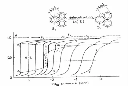
FIGURE 2.1 The phase diagram of Kr on graphite………..19

FIGURE 3.1 A molecular structure of graphene………..20

FIGURE 3.2 The synthesis of grapheme on nickel………..23

FIGURE 3.3 The phase diagram of Kr on graphite………..29

FIGURE 4.1 Quartz Crystal Microbalance (QCM)………..30

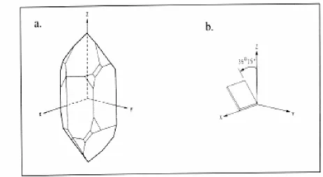
FIGURE 4.2 Quartz Crystal………..32

FIGURE 4.3 QCM while it’s oscillating in transverse shear mode………..33

FIGURE 4.4 Oscillating QCM with adsorbed film………...38

FIGURE 4.5 Oscillating QCM with adsorbed film in the presence of a surrounding gas...………….……….……….43

FIGURE 4.6 Different Stages of an Auger process in the atomic shells………..54

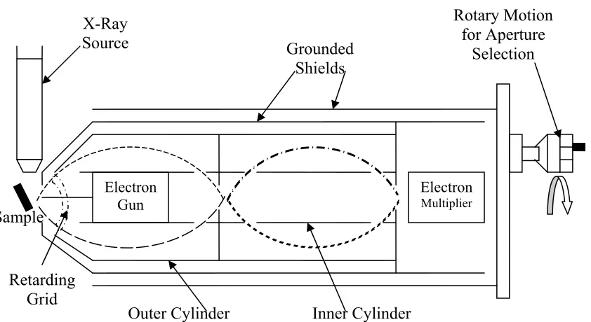
FIGURE 4.7 Double-Pass Cylindrical Mirror Analyzer used for AES and XPS…….56

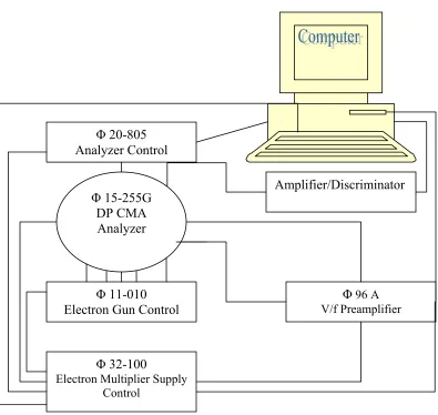
FIGURE 4.8 PC Interface and electrical connections of the double-pass CMA ESCA/AES………59

FIGURE 5.1 UHV System………...60

FIGURE 5.2 TELEMARK E-beam Evaporator………...62

FIGURE 5.3 Home-built Evaporator………63

FIGURE 5.4 Pierce oscillator circuit………64

FIGURE 5.6 Data Acquisition Electronics………..67

FIGURE 5.7 QCM Preparation………69

FIGURE 5.8 Auger Analysis of copper-coated QCM……….72

FIGURE 5.9 AES Analysis of ethylene on copper-coated QCM after annealing in experimental cell………..……74

FIGURE 6.1 QCM mass signal vs. pressure for krypton on graphene/Fe……..……75

FIGURE 6.2 Auger Spectrum of graphene on Fe after annealing...76

FIGURE 6.3 Mass uptake vs. Pressure of Kr/Ni………..…..78

FIGURE 6.4 Dissipation vs. Pressure of Kr/Ni………..…79

FIGURE 6.5 Mass uptake vs. Pressure and Dissipation vs. Pressure of

Kr/graphene/Ni………...81

FIGURE 6.6 Mass uptake vs. Pressure of Kr/graphene/Fe at 21mV………...82

FIGURE 6.7 Dissipation vs. Pressure of Kr/graphene/Fe (Linear Scale) at 21mV…82

FIGURE 6.8 Mass uptake vs. Pressure of Kr/graphene/Fe at 30mV………..83

FIGURE 6.9 Dissipation vs. Pressure of Kr/graphene/Fe (Linear and Log Scales) at 30mV…….………...………83

FIGURE 6.10 Mass uptake vs. Pressure of Kr/graphene/Fe at 37mV………..84

FIGURE 6.11 Dissipation vs. Pressure of Kr/graphene/Fe (Linear and Log Scales) at 37mV…....………84

FIGURE 6.12 QCM mass signal vs. Pressure of Kr/Au/graphene/Ni (Linear and Log Scales)………...85

FIGURE 6.13 Dissipation vs. Pressure of Kr/Au/graphene/Ni……….85

Log Scales)………86

FIGURE 6.15 Auger Analysis of nickel-coated QCM………...87

FIGURE 6.16 Auger Analysis of HOPG………88

FIGURE 6.17 Auger Analysis of graphene/Ni………...89

FIGURE 6.18 Auger Analysis of graphene/Fe………...90

FIGURE 7.1 Superimposed adsorption isotherms (one layer)……….92

FIGURE 7.2 Superimposed adsorption isotherms (multiple layers)………93

FIGURE 7.3 QCM Slip time of Kr on graphene/Ni……….94

FIGURE 7.4 T vs. “T+ ∆Tt” of the layer measured at a sliding speed of 2m/s……..100

CHAPTER 1: INTRODUCTION

Tribology is the discipline of science and technology concerned with the interaction of

surfaces moving relative to each other. It includes subjects such as friction, wear and lubrication. Tribology has significant social and economic impact. For example, it has been estimated that the USA alone incurs hundreds of billions of dollars per year in costs

related to tribology [1]. A recent boom in nanotechnology has accelerated the quest to understand tribological properties at the microscopic level including, a growing interest

to tribologically characterize miniature systems such as micro-electro-mechanical systems and computer hard drives. The heat energy associated with such systems is of great importance, as it may induce physical changes such as melting and/or chemical

reactions that completely alter the local surface properties.

1.1Sliding Friction at the Macro- and Atomic-Scales

When an object moves along a surface or through a viscous fluid or gas, it experiences forces that resist its motion. These resistive forces are called frictional forces. They are

non-conservative in nature. That is, the kinetic energy associated with the motion is irreversibly converted to heat. Therefore when an object moves along a surface of another

object, heat is dissipated at the interface of the two objects. This is usually accompanied by a temperature rise.

On the other hand, objects that are initially at rest can be made to be in relative motion by

the static force that kept the objects stationary and is called static friction. It is not associated with energy dissipation. The static friction Fs is given by

Fs≤µsN 1.1

where µs is the coefficient of static friction and N is the normal load.

In this dissertation, we present work exclusively related to kinetic friction and the temperature rise associated with it. In the supplementary part of this dissertation, we shall discuss, briefly, the reduction of friction of some systems through lubrication. Before

delving into the heat or temperature changes due to sliding friction or tribo-induced heating, it would be apt to give a somewhat brief description of the mechanisms of

friction in the first place.

A background description of some of the work involving krypton on graphite system and related systems will also be presented, as these relate to friction and/or heating or phase

changes.

The friction, Fk, of two objects in relative motion is often classically described at the

macroscopic level by familiar Amontons’s equation,

Fk = µkN 1.2

where µk is the coefficient of friction and the N is the normal load or force applied in

sliding contact. This force is generally independent of the apparent area of contact. The

French physicist, Charles A. Coulomb made another observation in the 18th century that the force is also independent of the velocity [2]. This had been dubbed the third law of friction. Attempts had been made by Coulomb to attribute the mechanisms of friction to

made to slide over one another they commonly stick together through friction and become cold welded. This obviously is the result of sufficient large friction for adequately smooth surfaces. Another example that demonstrates failure of surface

roughness as a fundamental mechanism for friction is household adhesive tape, which has relatively smooth surface but exhibits disproportionately large friction. Given these and

other anomalies observed at the macroscopic level, tribologists have long been attempting to nail down the mechanisms of friction at a nanoscale.

The availability of surface probe, lateral and atomic force microscopes and a host of other

diffraction and spectroscopy techniques has had a huge impact on the advancement of our understanding of the mechanisms of friction. However, more needs to be done to fully

understand the mechanisms and the effects of friction. The series of discoveries leading to the current advancement of our understanding of the mechanisms of friction by relating the contact area and the frictional force was kicked off in the 1950’s by Bowden

and Tabor in Cambridge [3]. They discovered that friction was proportional to the true contact area completely independent of the apparent contact area, which becomes pronounced at the macroscopic level. When two objects are in sliding contact their

contact regions are at their asperities. These asperities get worn out while others are formed. However, these regions of true contact are cumulatively much less than the

apparent area and would be microscopic in nature. For true contact area Ac with lateral

shear strength s at the contact region, the frictional force is F is given by

F = AcS 1.3

be discerned from the lateral stress as the friction changes due to changes in the normal load. After exploring this issue extensively Bowden and Tabor’s group at first believed that strong bonding at asperity contacts followed by wear was the physical mechanism

underlying friction [3]. However, this idea was disproved in the 1970’s by Tabor and Israelachvili. Israelachvili worked with a Surface Forces Apparatus (SFA) that he

adapted for frictional measurements. A picture and a description of the SFA are presented in section 1.3 of this dissertation. Using the SFA, Israelachvili and Tabor were the first to provide conclusive experimental evidence that friction could occur in the total

absence of wear. [4, 5]

In a paper published by Tomlinson in 1929, a model was given as to how friction is

generated at the microscale [6]. In that model, atoms in the vicinity of the moving surface respond to the motion by vibrating and these are called phonons or sound waves and it is these vibrations that are guised, at the atomic scale, as friction as they dissipate energy as

heat.

The concept of phononic friction was independently revisited by Sokoloff et al. in 1978, [7, 8] and McClelland and coworkers in the 1980’s, who re-derived models similar to the

original work of Tomlinson. McClelland, Mate and colleagues subsequently developed the Atomic Force Microscopy (AFM) for applications to studies of atomic scale friction

in an effort to detect phononic mechanisms for friction [9]. A picture and a description of the AFM are also presented in section 1.3 of this dissertation. The technique has proven to be a revolutionary new probe for studies of atomic scale friction in particular, and

The first experimental evidence of the existence of phononic friction came from work done with the Quartz Crystal Microbalance (QCM) and further modeling of such experiments. The QCM was first used by Widom and Krim for friction measurements in

1986-1988 after decades of its traditional use of microweighing [10, 11]. A description of how the QCM is adapted for friction measurement purposes is presented in section 1.3

whilst a fairly more detailed description of the QCM will be presented in chapter 4 of this dissertation.

1.2Frictional Heating and Temperature Rise at a Sliding Interface

It is not completely clear as to what the exact relation between the temperature rise at a

sliding interface and the sliding velocity is. Even though the heat rise is presumably due to friction which may be a result of both phononic and electronic excitations, efforts to try to relate the temperature rise at a sliding interface and the sliding velocity often prove

very difficult. On one hand, one might speculate that the heat and temperature rise might increase with sliding velocity since the frictional force generally increases with sliding velocity and hence work done by such an increasing force would increase. On the other

hand, one might think that the decreasing velocity arises in the first place due to increasing friction and as such would increase the frictional heating and temperature rise

at the sliding interface. These opposing views had been difficult to resolve since the temperature rise would depend, among other factors, on the surface properties of the sliding interface. Given that such an interface is buried, it presents so many transients and

of a macroscopic sliding interface shows a linear dependence of the temperature to the sliding velocity [12]

The primary aim of this dissertation is to conduct friction experiments on atomic-scale

systems that have known surface properties, so that they can be accurately modeled. We present QCM data aimed at examining the effect of changing sliding speed on the heat

generated and the temperature rise at the interface. The data are obtained from adsorption experiments performed on krypton on Ni(111), Fe(100), graphene/Ni, graphene/Fe and Au/graphene/Fe. In addition, we investigate the temperature rise as a

result of the oscillations in the course of the residence time.

Phononic friction arises as a result of the sliding induced excitation of atomic lattice

vibrations. In 1997, Tomassone et al. employed two numerical methods to measure the frictional forces in an adsorbed monolayer and assuming only phononic friction as the source of energy dissipation [13]. They simulated an adsorbed xenon monolayer sliding

on a Ag(111) substrate and compared their results to the frictional results of Daly and Krim who investigated xenon on silver via QCM experiments [14]. In their first approach, Tomassone et al. applied an external force on the xenon adsorbate at time t<0

that caused the adsorbate to slide across the silver substrate. The external force was then removed at t>0 and the slip time τ was determined from the resulting velocity given by

V(t) = Voexp(-t/τ ).

In many numerical studies involving temperature rise, a thermostat is used to regulate the temperature by adding or removing energy to the system to maintain a constant

related to friction by the fact that the adding or removing energy would inadvertently excite or damp the adsorbate film [13]. Damping from the thermostat would introduce an additional frictional force at the interface, which is undesirable since the only component

of friction that is of interest is the phonons. Therefore, in the technique employed by Tomassone et al., the thermostat measured the temperature for time t<0 and when the

system reached equilibrium the external force and thermostat were removed. This allowed for only phononic friction to slow the adsorbate. The highest temperature rise observed by Tomassone was 13K, which occurred for the largest value for the initial

velocities.

In the second method, a QCM experiment was simulated by having no external force

acting on the adsorbate. The QCM simulation is described by a linear response of the frequency and the substrate velocity as adsorbates are added to the film. This response, which defines the acoustic impedance, is thus related to the friction. There were no

interfacial temperature measurements in this method.

Both methods took the phononic friction into consideration and yielded results which agree well with the friction results of Daly and Krim. However, given the uncertainties of

what is known about the Ag(111) substrate corrugation, electronic effects could not be ruled out entirely. In studies involving graphite substrates, this may not be a critical issue

since such systems are described by substrate potentials that are extremely well characterized.

Sliding interfaces are generally inaccessible and therefore pose a great challenge in the

friction at a sliding interface generally employ a thermostat to measure the temperature. However, the thermostat has a damping effect on the system and thus introduces another component of friction to the measured value [13]. To get around the problem, researchers

had traditionally allowed the system attain thermal equilibrium and then turn off the thermostat. This technique allows the friction to be measured while the temperature is

estimated/assumed but the temperature values obtained from such techniques range from thousandths to tens of degrees [14]. Therefore a precise measurement of the effect of sliding at the interface requires some knowledge of the temperature at the interface. A

Kr/graphite system, or KGS for brevity, has a well documented isotherm from which we could infer the temperature of the interface.

An obvious concern with the picture so far painted of friction and sliding is that the friction is there to oppose the relative motion in the first place. Therefore if a fairly atomically rigid surface slides over another with some friction accompanied by heat rise,

could the heat rise be entirely attributable to the friction? Well, not quite – as the sliding could also contribute some of the kinetic energy to internal energy which would effective raise the temperature. For example if we look at a motion involving extremely low

coefficient of friction, the sliding would be fairly smooth and associated with high kinetic energy giving rise to high slip time but also high temperature as the kinetic energy gets

converted to heat at the surface. Likewise if the motion involves extremely high coefficient of friction, the frictional force would be fairly high. This could be accompanied by a heating of the surface and temperature rise. So, one of the prime

on a monolayer of graphite, called graphene. We then relate the effects [of sliding] to the two-dimensional phase transitions:

1. solid-liquid

2. commensurate-incommensurate

We would also establish the effect of atomic spacing of the graphene on the sliding

friction.

1.3 QCM, AFM and SFA Techniques – An Overview

Here we will provide a brief description of how the QCM is adapted for friction measurement purposes. A more detailed description of the QCM is given in chapter 4 of

this dissertation. A QCM consists of a single crystal of quartz that oscillates in transverse shear mode with some resonance frequency and negligible internal dissipation. That is, the temperature rise within the crystal due to the shear oscillation is extremely low. For

the work described in this dissertation, crystal frequencies were generally 5, 6 and 8MHz. The oscillations are generated and sustained by an external alternating voltage applied to the thin metal electrodes deposited on the major faces of the quartz. Atomically thin films

later adsorbed onto the QCM electrodes produce shifts in both the frequency and the quality factor Q, which are indicative of the degree to which the films are able to track

the oscillatory motion of the underlying substrate. The friction for this geometry is characterized by the viscous friction law, given by

F = mv/τ 1.4

1/e of its initial value. A short hand name for τ, for the purpose of tribological argument

is, slip time. The slip time is related to the friction coefficient, ηby the equation

η = ρ2/τ 1.5

where ρ2 is the mass per unit area of the adsorbate. However, the slip time is related to

measured quantities such as frequency and amplitude through the equation

δ(1/Q) = 4πτ(δfo) 1.6

where δfo and δ(1/Q) are the frequency and inverse quality factor shifts, respectively. The

quality factor, as we shall show later, is proportional to the amplitude of the oscillation. Two other tools that serve as prudent tools for nanotribology research are the Atomic Force Microscopy (AFM) and Surface Force Apparatus (SFA) with the former providing

the more obvious connection between nanotribology and conventional tribology. While macroscopic sliding parts almost always maintain contact through countless microscopic

asperities, AFM utilizes a single probe of nanometer-scale sharpness to form tactile images of open surfaces. Therefore the AFM probe represents the smallest possible fragment of a typical sliding interface which is an individual asperity. AFM has already

proven useful in establishing that the motion of individual asperities over even the smoothest available surfaces is not smooth, but of the ``stick-slip'' type. A current

Figure 1.1 Atomic Force Microscope (AFM) schematic. The image at left is a lateral force image of MoS2 taken from [16]. In contact AFM mode, the AFM tip is brought into contact with the sample surface, and then raster scanned across the sample surface. The AFM tip maintains contact with the sample, and the AFM cantilever moves in response to the sample's morphology and frictional forces between the sample and the AFM tip. A laser beam is reflected off the back of the AFM cantilever and onto a four-quadrant photodiode. In this way, small angular motions of the cantilever can be detected. The position of the laser beam on the photodiode provides both a map of the sample surface and a friction measurement.

The surface forces apparatus (SFA) [4, 5] may be considered an intermediate instrument

between AFM and QCM and is suitable for studying atomically flat, molecularly thin films between excellently characterized mica planes. For example, SFA permits the sensitive measurement of forces between curved, crossed mica surfaces contacting over

an area a few microns wide. Mica is a uniquely useful substance for surface science--particularly nanotribology--being easily cleaved to form atomically flat planes as much as

“confined” we are essentially saying that the films are held within a tight space not much larger than a constituent molecule of the film. Interestingly enough, confinement routinely produces effects we will not expect to see in films adsorbed on open surfaces.

A current disadvantage of SFA work is the difficulty encountered in implementing SFA under clean (UHV) conditions.

Figure 1.2 Diagram of a Surface Forces Apparatus (SFA) experiment from [17]. The coiled springs are representative of any device used to measure the normal and shear forces between the samples. The SFA makes use of two cleaved mica surfaces, which are among the smoothest surfaces known. Investigators can place lubricant films, which can be as thin as a few molecules, between the mica surfaces and slide them about, to see how the films affect the friction.

1.4 Why Use QCM?

Given the disadvantages that shroud the use of either the AFM or SFA, there seemed to be real need to explore an alternative friction measurement device, thus, the QCM. The

uses include, but are not limited to, the study of sputtering, oxidation, catalysis, and physical adsorption. In almost all of these cases, the surface being studied serves an additional purpose as an electrode of the QCM.

The application that gave rise to the current use of the QCM in nanotribology is the study of inert gas adsorption on metals [15]. Originally, adsorption studies were limited to

adsorbent materials of remarkably large surface area - graphite, h-BN, materials that also happen to be lubricants--in large quantities. QCM techniques permit the study of physical adsorption on a larger number of substances. The subject of physical adsorption

deserves a chapter of its own. For now, let us just point out that the study of inert gases on QCM electrodes preceded the study of sliding inert gas films by several decades.

The bulk of this dissertation involves friction studies on graphene instead of graphite. The latter, it though offers unique opportunities for surface science studies, is incompatible with the QCM for friction studies. Graphene can, however, be grown on the QCM.

Commercially available graphite samples which are placed on the QCM would completely fail to produce direct response due to the oscillatory motion of the QCM. This is because the QCM is sensitive to mass loading under 1% of an atomic layer thick - so

long as the adsorbate covers the active area of the QCM and that the adsorbate can be securely coupled to the active area of the QCM. This requirement of a securely coupled

surface for QCM studies turns out to be a severe constraint. The active area of a typical QCM experiences a peak acceleration on the order of 107m/s2. We may not, under normal laboratory conditions, glue an ideal surface like graphite to the QCM and expect

CHAPTER 2: PHYSICAL ADSORPTION

Before we delve into the main analysis of the results we will describe surface adsorption processes and relate them to the phase diagrams and phase transitions of interest to the

work presented here.

2.1 Chemisorption and Physisorption

In chemisorption, a strong 'chemical bond' is formed between the adsorbate atom or

molecule and the substrate. In this case, the adsorption or binding energy, ∆Hads, of the

adsorbed atom is likely to be a good fraction of the sublimation energy of the substrate,

and sometimes could even be more. For example, ∆Hads = 3.2 x 10-19J for an adsorbed

atom on an fcc (100) surface when the sublimation energy is about 4.8 x 10-19J for a case

of a substrate and 'adsorbate' of the same atom. So, energies of a few eV/atom are typical of chemisorption with adsorbed atoms usually residing on the surface for quite a long time.

Physisorption is weaker, and is often characterized by much shorter residence time than the chemisorption residence time. However, a better distinction is that in physisorption,

the energy of interaction is largely due to the van der Waals force. This force is due to fluctuating dipole moments on the interacting adsorbate and substrate, and is present between closed-shell systems. Typical systems are inert gases on lamellar surfaces.

Adsorption of molecules often proceeds in two stages. A first, precursor stage, has all the characteristics of physisorption, but this state is metastable. In this state the molecule may re-evaporate, or it may stay on the surface long enough to transform irreversibly into a

chemisorbed state. This transition is rather dramatic, usually resulting in splitting the molecule and adsorbing the individual atoms: dissociative chemisorption. The adsorption

energies for the precursor phase are similar to phyisorption of rare gases, but may contain additional contributions from the dipole, quadrupole, etc moments of the molecules. The dissociation stage can be explosive- literally. The heat of adsorption is given up suddenly,

and can be imparted to the resulting adatoms [18].

About a century ago, Langmuir proposed a model in which adsorbates were bound to the

adsorbent surface at specific sites only. These adsorptions were marked by uniform binding energy. In addition, Langmuir proposed that subsequent gas particles attempting to impinge or adsorb on occupied sites will rebound into the gas phase. Thus, only one

monolayer is formed and any surface interaction or diffusion of adsorbates is excluded. The Langmuir Adsorption Isotherm thus results and such an isotherm is used to calculate

the fraction, θ, of a surface covered by an adsorbed layer in thermal equilibrium as a

function of vapour pressure p. That is, the Langmuir isotherm is given by:

θ = C1χ(T)p/[1+χ(T)p], with χ(T) = C1-1exp(∆Hads/kT)

where C1 is a constant and can be shown to be equal to kT/qλ3_{, ∆H}

ads is the adsorption energy and k is Boltzmann's constant.

The fractional coverage starts out linearly proportional to ambient pressure at low pressure and asymptotically approaches unity at high pressure.

Alternatively, one can, however, assume that all the particles adsorb independently of one

another. This is a nonlocal adsorption whereby adsorbates are free to move around. This

implies that the adsorption energy, ∆Hads and consequently the residence time, τa are

independent of the surface population, Na. This model, known as Henry’s law, is relevant

to systems with very weakly bound adsorbed particles. Hence, the Henry's Law for 2D gas adsorption is given by:

Na/A = χ'(T)p, with χ'(T) =C2-1exp (Eo/kT),

and C2 = kT/qzλ.

One of the main shortcomings of the Langmuir model is that it explicitly forbids the possibility of adsorption beyond a monolayer. Since adlayers with many atomic layers

thick are not uncommon in physical adsorption systems, Brunauer, Emmett and Teller had, since 1938, modified gone a step beyond the Langmuir. Their model is the so-called

BET model and it allows for the possibility of multilayer adsorption and becomes and very powerful tool for determining surface areas.

When adsorption of atomic or molecular particles takes place on a substrate, heat is

evolved. This heat is usually accompanied by temperature rise felt at the interface. With the use of a high precision heat detector, the temperature can be measure to the order of

thousandth of a degree.

The heat of adsorption is, however, often determined by desorption in which energy (desorption energy) is supplied to break the bond between the adsorbate and substrate

substrate type as well as the temperature of the interface. This naturally leads one to ask: how long does an adsorbate (atom, molecule, or the group thereof) stay on a surface at a particular temperature before desorbing assuming some heat of adsorption between the

adsorbate and the surface and where the heat of adsorption is directly related to the activation energy? This length of time is indeed the adsorption time or residence time and

is linked to the formation of two dimensional phases. There is a remarkably low activation energy for transport of adsorbate along the surface of the adsorbent. The surface activation energy, usually within less than half the bulk activation energy gives

rise to diffusion and exchange of adsorbed particles from one site to the other along a plateau or facet. These exchanges (movements) are so high that one may generally

assume equilibrium among the adsorbates in the various substrate sites, hence long residence time, τa given by:

τa = τoExp(∆Hads/RT)

where τo is correlated with the surface atom vibration times and is in the order of 10-12

sec, ∆Hads is the heat of adsorption per mole of atoms, T is the temperature of the surface

in Kelvin and R is the universal gas constant. Using the fact that ∆Hads = 12.97kJ/mol of

Krypton [19] and T (liquid nitrogen temperature) = 77K, we obtained an average residence time of about 6.3x10-4 sec. So for appreciably long residence time, one may

regard the surface as a two-dimensional phase.

Small range of transition pressures may sometimes be attributable to facet size effects. In a paper published in 1979, Larher argued the formation of two-dimensional adsorbate and

the extent of these adsorbates [20]. Using the volumetric adsorption isotherm measurements of argon adsorbed on CdCl2, Larher estimated the critical exponent value

of β = 0.16. This quantity, which appears in the relation giving the change in the adsorbed quantity during a coverage transition as a function of deviation from the critical temperature, reflects the two-dimensional character of the transition. In addition, he

obtained No (∂logP/∂N)T value of 0.005 which corresponds to a change in the chemical

potential from the bottom to the top of step less than 7J/mol for a process involving an

energy change of about 8kJ/mol. Thus, Larher claimed the presence of first-order transition. For such a variation in chemical potential, µ, arising from a range of facet sizes from r to ∞, a reasonable facet size of about 600Å was obtained using the relation:

µ(r) – µ(∞) = Aσ/r

where A is the molecular area and σ is the line tension.

2.2 Phase Diagrams and Phase Transitions

One of the intriguing aspects of both physi- and chemi-sorption is the large number of phases that can exist at the surface, and the transitions that occur between these phases. There is a comparable richness of structure to that displayed in high pressure physics,

where there is both a density ρ, and a corresponding structure, at a given p and T. The

relation ρ = f(p,T) is called the equilibrium Equation of State (EOS) in the (3D) physics

of bulk matter, or the (P,V,T) relation and the corresponding equation in 2D is given by θ = f(p, T) or θ = f(µ, T)

where µ= kT ln (p).

Therefore if a 2D gas layer is compressed by increasing the gas pressure p, the gas adsorbed particles come together within their mutual interaction forces described by Lennard-Jones potential. Consequently, phase transitions may take place as the coverage

increases from a monolayer to few monolayers.

2.4

There have been increasing experimental and theoretical interest in various properties of atoms and molecules (of gases) physisorbed on graphite surfaces.

Since the physisorbed atoms and molecules can exist in a variety of thermodynamic

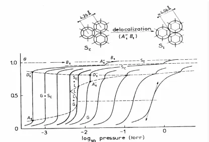
phases, of particular interest are the thermodynamic phases and the associated transitions of adsorbed Kr on graphite surfaces. The phase diagram [volumetric adsorption isotherm]

for such a system is shown in figure 2.The diagram (isotherms) indicates the existence of two dimensional gas, liquid and two solid phases [18]. The curves represent the volumetric adsorption isotherms for Kr/Graphite at 77.3K to 109.5K at sub-monolayer

coverages.

CHAPTER 3: GRAPHENE

So, one of the prime objectives of this dissertation is to determine the effect of temperature or heat rise at the sliding surface. In particular, we look at the temperature

changes due to sliding krypton on a monolayer of graphite, called graphene. We then relate the effects [of sliding] to the two-dimensional phase transitions:

3. solid-liquid

4. commensurate-incommensurate

We would also establish the effect of atomic spacing of the graphene on the sliding

friction.

3.1 Graphene Properties

Figure 1 shows the molecular structure of graphene. It is a single planar sheet of graphite and has sp2 bonded carbon atoms. These atoms are densely packed into a benzene ring (hexagonal) structure and terminated by hydrogen giving a typical molecular formula of

C62H20 with lattice spacing equal to 0.246nm. Graphene is typically chemically inert due to the fact that its surface is covalently terminated, thus allowing graphene to be kept

clean under vacuum. It also has a relatively large surface area which makes it a viable candidate for use as a lubricant. Another property of graphene which makes it an ideal surface for surface science studies is its flatness. Graphene can be synthesized to form an

atomically flat surface such that surface analytical techniques requiring diffraction to correctly characterize surface crystallography and other atomic scale surface properties

can be carried out. Graphene, even though looks like a huge molecule, serves as a

theoretically and experimentally simple model for graphite. Therefore any studies carried out on graphite with the consideration of only the outermost layer by virtue of the weak

van der Waals interaction between layers is effectively applicable to graphene. Other properties of graphene that make it a unique material for use in various technological applications are its high conductivity and remarkably flexibility and strength. Graphene

had garnered attention due to its use for producing other fascinating materials like fullerenes and carbon nanotubes renowned for their unique properties. Carbon nanotubes,

for example, could be thought of having graphene as a basis in which the graphene sheet had been rolled up to form a cylindrical structure, hence, a nanotube. Therefore, any of the several applications currently considered for carbon nanotubes could be applied to

storage media for molecular hydrogen and very importantly, protective coating for devices.

The existence of a two-dimensional phase consisting of gas, liquid and solid layers has

been shown in a Kr-graphite system at sub-monolayer coverages. The natural Kr-Kr interatomic spacing is a few percent smaller than the interatomic spacing of the

second-neighbour graphite cells. However, in such systems, the corrugation of the Kr-graphite potential is sufficiently large that the Kr atoms are held in these cells to form commensurate monolayer. This may, however, undergo a phase transition to form a

denser incommensurate layer and this layer exists over an appreciably wide range of temperature and pressure before a second Kr layer condensation sets in. The transitions

of such phases due to changes of the thermodynamic effects are called the thermal phase transitions. Moreover, there are two solid phases which are commensurate and incommensurate with respect to the underlying graphitic surface. Likewise

thermodynamic effects can bring about transitions between phases and called structural phase transitions. In this work we had attempted to address the transitions of these two types of phases by investigating the temperature rise at the interface. In particular we had

looked at the solid-liquid interface. The solid-liquid transition is of prime importance because it signifies a second order transition at relatively high coverages and as such

3.2Graphene Synthesis

In this section, we present the detail description of the different procedures employed to synthesize graphene. The processes involve the catalytic decomposition of CO to C and

CO2 as indicated by the chemical reaction

2CO → C + CO2

Figure 3.2Illustration of the Synthesis of Graphene on Nickel[21]

Figure 3.3shows the schematics of the physical set-up to synthesize graphene on nickel. The nickel substrate which acts as a catalyst is kept at 500o_{C while CO gas at pressure of}

about 10-6 Torr is dosed on it surface. This produces intermediate NiC and CO2 products. The CO2 quickly returns to the gaseous phase while the nickel carbide is further broken

Gas Source: CO at 10-6Torr

Intermediate Products: NiC and CO2

Final Products: Graphene

Catalyst: Nickel at 500oC

CC CCCOO O OC O C O C C C C C C C C C C C

down into pure carbon and nickel. The carbon forms a graphitic layer (coating) on the metallic nickel and inhibits further reaction. This process thus poisons the metal and prevents it from being used as a catalyst to form nickel carbide. Other metals that could

be used as a catalyst to yield the same products are iron and cobalt. However, graphene synthesized on different metal substrates and conditions produce different lattice spacing.

For the purpose of this study, we had employed two different metals, namely nickel and iron, to serve as catalysts for the carbonizing or coking procedure. In addition, the typical temperature for coking in our studies is 350-400 oC.

3.2.1 Graphene/Fe(100)

The Fe (100) electrode was prepared in UHV at room temperature by slowly depositing iron on the major faces of a QCM via e-beam evaporation of iron rod at an average rate of 12Å/min. Typical Fe thicknesses used for this study are in the range of 1000 - 1500 Å.

The sample was then transferred to the heating stage and was annealed to 375˚C. The graphite monolayer was formed on the Fe(100) surface by cracking carbon monoxide (CO) at a sample temperature of 375˚C while exposing it at a pressure of low 10-6_{Torr for}

10 minutes. The corresponding Auger spectrum displayed the characteristic graphite line shape.

3.2.2 Graphene/Ni(111)

The Ni (111) electrode was prepared in UHV at room temperature by slowly depositing

sample was then transferred to the heating stage and was annealed to 400˚C. The graphite monolayer was formed on the Ni(111) surface by cracking carbon monoxide (CO) at a sample temperature of 400˚C while exposing it at a pressure of 10-6Torr for 10 minutes.

The corresponding Auger spectrum also displayed the characteristic graphite line shape as in the Fe system.

3.2.3 Au/Graphene/Ni(111)

An overlayer of gold of a thickness of about 6 Å was deposited at room temperature on

the monolayer graphite/Ni(111) via thermal evaporation of molten gold pellets on a tungsten boat. The gold was allowed to evaporate at stable rate before the QCM bearing

the monolayer graphite/Ni(111) was introduced in the field of the evaporating gold and was removed from the field as soon as the desired thickness was obtained. The sample was then transferred to the heating stage where it was annealed to 375˚C and then

transferred to the experimental cell. AES spectrum shows the presence of graphitic line shape and adsorption isotherm indicates steps occurring at about 28.6Hz. These seem to confirm that the annealing of the sample allows the intercalation of the gold atoms

underneath the graphite monolayer and the restoring of a graphitic overlayer [22].

Table 3.1 shows the different lattice spacing that could be obtained from different

preparation condition. Notice that one can conceivably alter, by about 2%, the lattice spacing of graphene synthesized on nickel by intercalating it with few monolayers of gold. This, therefore, permits us to be able to tune graphene to the desired lattice

Table 3.1. Display of the different lattice spacing of graphene synthesized on different metal substrates.

System Lattice Spacing (nm)

Graphene/Ni 0.251

Graphene/Fe 0.246

Au/Graphene/Ni 0.246

3.3 Selected Works on KGS-related Systems

In this section a brief description of some of the works related to krypton on

systems is given.

In a Quartz Crystal Microbalance (QCM) study published in 1991 by Krim, Solina, and

Chiarello, measurements of the friction of krypton monolayers sliding on high quality Au(111) surface were reported [23]. Krypton adsorption isotherms carried out at 77.4 K by submerging the adsorption chamber in a liquid nitrogen bath and allowing it to come

to equilibrium were reported. At 77.4 K, krypton condenses as a uniform film to within 2 atoms thick. The gas first condensed to a liquid and then solid as the pressure increased.

A frequency shift of 10.4 Hz was observed which translated into about 0.066 atoms/Å2 of film coverage for a 5 MHz Au crystal. This is consistent with a liquid monolayer. They

0.078 atoms/Å2 film coverage and it was actually the solid phase coverage. This liquid-solid phase transition occurred at 1.45 Torr. They then compared the slip times before

and after the phase transition for Kr/Au(111), and found that solid krypton monolayers sliding on Au(111) had slip times five times larger than liquid monolayers of krypton. These results can be translated into a simple language to describe the surface as “slippery

when dry!”

In 1994, Cieplak, Smith, and Robbins modeled these using standard molecular dynamics simulations [24]. They modeled mobile krypton atoms on a perfectly rigid gold

substrate. The gold substrate provided a fixed periodic potential that acted on the adsorbed krypton layer. The krypton-krypton interactions were modeled with the

standard 12-6 or Lennard-Jones potential:

V(r) = 4ε[(σ/r)12 _{– (σ/r)}6_{] 3.1}

Where r is atomic separation and ε = 17 meV and σ = 0.357 nm are characteristic energy

and length scales for krypton, respectively. The krypton-gold interaction potential was

modelled with a formula by Steele for a Lennard-Jones adsorbate on a rigid substrate or adsorbent [25]:

Vs(x,z) = ε’[Vo(z) + fV1(z) Σi cos(Gi• x)] 3.2

Here x is the position within the adsorbent plane, z is the distance above the first layer of substrate atoms, Vo is the average potential energy between adsorbate and adsorbent, V1 describes the changes in adsorbate/adsorbent potential with respect to adsorbate position

and Gi are the reciprocal lattice vectors and f is a scaling factor introduced by Cieplak et

adsorbate position Using the above model, they determined the frictional force in two ways:

1. they applied an alternating force to the adsorbates which were then set into

oscillation thus simulating the oscillating QCM experiment, and then measured the adsorbate velocity and

2. they applied a constant force to the adsorbates and then measured the adsorbate velocity

In both instances, they found that the solid krypton layer slipped longer on the substrate

than the liquid. Thus the Krim et al experimental findings of 1991 were reproduced. There have been increasing experimental and theoretical interest in various

properties of atoms and molecules (of gases) physisorbed on graphite surfaces.

Since the physisorbed atoms and molecules can exist in a variety of thermodynamic phases, of particular interest are the thermodynamic phases and the associated transitions

of adsorbed Kr on graphite surfaces. The phase diagram [volumetric adsorption isotherm] for such a system is shown in figure 3.3.The diagram (isotherms) indicates the existence of two dimensional gas, liquid and two solid phases [26]. The curves represent the

CHAPTER 4: EXPERIMENTAL TOOLS

4.1 QCM – General Description

The quartz crystal microbalance, QCM, had been around for quite a while as a

microweighing device. It is a precisely cut slab from a natural or synthetic crystalline structured SiO2 that has solid-solid phase transition at 573oC. We used the α-Quartz

which is the form below the transition temperature for microbalance applications. They exhibit excellent piezoelectric behavior. This means that electric potential is generated by exerting pressure (or mechanical strain) on the quartz crystal. Conversely mechanical

strain could be generated by applying alternating electrical potential across a piece of quartz crystal. This relation is linear for small strains and applies to about 2/3 of the

crystalline structures and for many polycrystalline pole materials [27].

Figure 4.1 shows the QCM used in this study. It consists of a thin disk of single quartz crystal with thickness in the order of a millimeter.

(b) shows the thickness of the QCM which is a thin quartz disk. (c) An alternating voltage applied to the leads causes the QCM to oscillate in a lateral shear mode or along the thickness of the disk.

The two major faces of the quartz disk are plated with metal electrodes which are connected to an electrical feedthru by means of metal tabs. These tabs, with the addition

of Ag paint, provide good electrical contact and mechanical support. The quartz also has a relatively high quality factor, about 105 and is very sensitive to very small masses

adsorbed on its electrodes. In fact, masses as small as 1pg/cm2 can be detected by the quartz.

In this work we had focused on the use of QCM as a probe for sliding friction, a

technique that was developed in 1986-88 by J. Krim and Widom [28]. They were able to show, with the use of acoustic impedance calculations, that if the shear stress between the

film and the QCM surface is below 103 N/m2, then the film will slip on the QCM surface enough to be detected by monitoring the changes in the QCM resonance frequency and amplitude.

4.2 The Quartz Crystal Microbalance - Cut

There are, however, different types of crystals depending on the cut. The first type is the so called Curie or X-cut. This type of cut has its face perpendicular to the X-axis and exhibits oscillations in the longitudinal direction along the Y-axis when an electrical

potential is applied along the X-axis. There is also the Y-cut which has its face perpendicular to the Y-axis. Electrical potential applied along the Y-axis generates

experiments requiring thermal stability usually proved difficult using these cuts, especially the X-cut. However, advances have been made on the Y-cut by producing rotated Y-cuts. In these modified cuts, the rotation of the Y-cut about the X-axis is varied

thereby making the frequency response to temperature changes virtually zero in the range of temperature -200oC to +200oC. When the rotation angles are made to be 35o 15’ and

-49o, AT-cut and BT-cut are obtained respectively. Figure 4.2illustrates the assignment of axes to a crystalline quartz and a specifically AT-cut crystal. The Z-axis is known as the optic axis, and the X- and Y-axes as the electrical

Figure 4.2. A schematic of the quartz crystal showing (a) axes of the crystal and (b) the AT-cut crystal

and mechanical axes, respectively. The piezoelectric effect is heavily directionally dependant and has to do with the forces and fields applied along the X- and Y-axes only.

Therefore, the quartz crystal should be cut at a specific crystallographic orientation and produce the proper shape. In fact, slight variations in the cut of a quartz disk can generate major effects on the frequency, stress and temperature responses of the quartz.

The AT-cut exhibits zero temperature dependence on the frequency, has a very high mass sensitivity, high frequency stability and remains the most used cut for transverse or shear

mode oscillations.

The BT-cut usually requires half as much more AT-cut quartz to produce oscillators. Due to their wide availability the AT-cut crystals were used for all the work

described in this thesis. Figure 4.3shows the shear oscillation mode of the AT-cut QCM.

Figure 4.3. Side view of QCM while it’s oscillating in transverse shear mode. The applied alternating voltage causes the faces of the QCM to move laterally in opposing directions.

~

QCM

Metal Electrode Adsorbed Film

4.3 Mass Loading and Frequency Shifts

The quantitative relation between mass loaded on the quartz and its vibrational frequency was first investigated by Sauerbrey [29].

Consider an AT-cut crystal with thickness t oscillating transversely as a result of an alternating voltage applied across its major surfaces. This oscillation would be that of

standing waves of wavelength λif

t = n λ/2 4.1

where n = 1,2,3…and

0

f λ = vq

where vqis the speed of wave propagation in quartz.

For the fundamental frequency, n = 1 and

f₀ =vq/2t 4.2

The addition of a small amount of mass of film, mfilm << mq, could be considered a direct

change in the thickness of the crystal and effectively a small perturbation on the quartz crystal’s mass. Therefore the change in frequency is given by

In terms of the mass of the quartz, the above equation can written as

and m_q = ρ_q At

0

0

dt

df

f = − t

0 q

0

dm

q

df

f = − m

4.3

Obviously, this change in the mass of the quartz is due to the mass of the added film mfilm on one side of the crystal.

Therefore

dfo = - m / ρq At ,

for an evenly distributed film on the active part of the quartz. Using equations (4.2) and (4.3), equation (4.4) now becomes

∆ f = -2 fo2(mfilm/A) /ρq vq

Now ρ_q = 2.65 g/cm3 and vq = 3.34 x 105 cm/s and for all the experimental work

described in this thesis mass adsorption on both sides of the crystal were considered. We therefore multiply the right hand side of equation (4.5) by 2 and plug in the constants. Thus, we obtain:

This equation gives a quantitative relation between the change in the resonant frequency of the crystal and the monolayer of a film that (1) uniformly covers the active area of the

quartz crystal, (2) perfectly adheres to the quartz crystal such that the film can track the oscillations of the quartz crystal, (3) is non-dissipative and (4), that has a mass that is

much smaller than the mass of the crystal.

Therefore using equation (4.6), one could compute the frequency shift corresponding to one monolayer of an adsorbate of known density on a quartz crystal of

6 2

0 4.52 10 mfilm

f f

A

−  

∆ = − × _{ }

  4.6

known frequency. For example, using an 8MHz crystal, the frequency shift for one monolayer of Kr, ∆f = - 26.6Hz; for Xe, ∆f = -37.1Hz and for TCP, ∆f = -27.2Hz.

4.4 The Quality Factor

Mechanical and electrical oscillating systems routinely employ the use of a

quality factor, Q. It is a dimensionless quantity that has been used to represent the degree of damping of the oscillator. It is defined as:

Acoustic energy is stored in the system by the driving mechanism and it is

dissipated due to internal friction and external damping forces whose effects are felt in the resonant frequency too. From the definition of the quality factor, it is clear that it is

inverse is the dissipation factor or the resonance bandwidth. That is, Q ~ D-1. Therefore, a high Q means low acoustic energy losses, high frequency stability and precise determination of the resonant frequency. This property of the quartz crystal renders it as

an ideal weighing device capable of detecting extremely small mass changes in a broad range of applications. The maximum attainable quality factor of a crystal depends on the

diameter and surface curvature of the blank quartz and is inversely proportional to the frequency of oscillation.

When a mass adsorbs on the quartz crystal the resultant dissipation is just the sum

of the individual dissipations in the mass plus the quartz crystal. Therefore the inverse total quality factor is given as the sum of the inverse quality factors of the mass and the

quartz crystal:

Energy stored in one cycle 2

Energy lost in one cycle

Changes in the quality factor are generally monitored through changes in the amplitude of oscillation of the quartz crystal caused by the addition of mass. As more mass adsorbs, acoustic energy losses in the material increase and the quality factor decreases further.

However, when the overall quality factor becomes exceedingly low, the oscillation of the quartz crystal will not be sustained and the crystal will cease to function.

4.5 Sliding Friction Measurements

In this section, we discuss how the QCM could be used to study the interfacial

sliding. This technique, developed by Krim and Widom [28], relies on the fact that a solid substrate is sliding back and forth with a film atop of it, undergoes interfacial slippage

and thus sliding friction, and, in general, the interfacial slippage and the sliding friction could be measured. This is achieved by relating the acoustic impedance presented by the film to the substrate motion to the interfacial slippage.

4.6 Acoustic Impedance

4.6.1 Acoustic Impedance of a Viscous Film (3-D fluid)

A standard problem in classical hydrodynamics is the acoustic impedance of

viscous fluid. Consider a film of thickness d, with bulk density ρ_3f and bulk viscosity

, 3f

η lying on a flat, solid surface as in Figure 4.4.

1 1 1

q m

Figure 4.4. Oscillating QCM with adsorbed film. Acoustic waves propagate into the film and dissipate energy.

If the solid surface undergoes a simple harmonic motion its velocity can be given by

u(t) = uoe-iωt

Now, taking the z-direction to be perpendicular to the solid surface, and the x-direction to be parallel to the motion of the surface, the motion of the solid surface will

cause shear waves to propagate through the film and the loading of the film can be described by the linearized Navier-Stokes equation for a viscous, incompressible fluid [29]

~

QCM

Metal Electrode Adsorbed Film z

x

( )

( )

x x

3 3 2

, ,

f f

z t z t

t z

υ υ

ρ ∂ = η ∂

where

υ

( )

solid surface. (where the subscripts 2 and 3 refer to surface and bulk values respectively,

while f and v will refer to the film and vapour phases.) Assuming that the film does not slip on the solid surface vX (z= 0,t) – u(t) = 0, and that its upper surface is free to move without any resistive force, the solution to equation (4.9) is given by:

where the dispersion relation is given by k = (iωρ/η)1/2 = (1+i)(ωρ / 2η)1/2. The stress

tensor component σzy describes the viscous fluid force per unit area applied by the fluid

to the plane and is given by

σzy = η(∂v/∂z)z=0.

σzy = ηku(t)tan(kd)

The acoustic impedance, Z = σzy / v, presented by the film to the motion of the solid plane

is given by

The resistive (or real) component R is proportional to the energy dissipation, while the reactive (imaginary) component X of the expression above is proportional to the inertia of the oscillator.

Stockbridge [30] was able to show that for a QCM whose two electrodes are exposed to the mass deposited the total quality factor and frequency shifts of the QCM

( )

x

cos ( )

, ( )

cos( )

k d z z t u t

kx

υ = −

3 2

3

3

tan( ), f

f f f f

f

Z R i X η k kd where k i ωρ

η

= − = =

4.10

are related to the resistive and reactive components, respectively,. of the total impedance presented to it according to the relation:

where

ρ

For very thin films, kd 〈〈1, the dissipative part of equation (4.10) vanishes and

the acoustic impedance reduces to just the reactive component given by

Sauerbrey's result for the mass-frequency relationship, i.e. equation (4.5), is readily

obtained if this result is substituted into equation (4.12).

4.6.2 Acoustic Impedance of a 3-D Vapour

The acoustic impedance presented to the quartz crystal changes when the crystal is transferred from vacuum to a gaseous environment. This change is due to the shear

impedance of the gas, and mass uptake if the gas adsorbs on the quartz crystal. In this subsection, we will attempt to present the quantitative measure of the shear impedance of the quartz crystal in the presence of the surrounding gas with given shear impedance.

4 2

1

,

tot tot

q q q q

R X

Q t t

δ δω

ωρ ρ

 

= =

   

3 2 , | | 1

f f f f

Z = − i X = −iωρ d = −iωρ for kd <<

4.12

We first consider the case when the gas does not adsorb on the quartz crystal. The

acoustic impedance of a purely viscous gas (with bulk density ρ3v and bulk viscosity η3v)

is found to have equal reactive and dissipative components given by [31]

where f is the frequency of oscillation.

The reactive loading of the gas is equivalent to an increase in inertia of the

oscillator and leads to frequency shifts which could be calculated by substituting equation (4.14) into equation (4.12):

At low pressures, the relaxation time τ _r of the gas particles after collision with

the vibrating crystal is of the order 2 x 10-7 seconds and thus becomes commensurate with the period of oscillation. The gas therefore is no longer a simple viscous fluid but

behaves as a viscoelastic gas with an unrelaxed shear modulus of elasticity. Its viscosity becomes a function of frequency and is given by[32]

3 3 0 2 v v q q f f f v πρ η δ πρ = * 3 3 1 v v r i η η ωτ = + 4.14 4.15 4.16 3 3 (1 )

v v v v v

The solution of the classical problem of the propagation of shear waves of the

viscoelastic gas yields the acoustic impedance *

v

Z of the viscoelastic gas is then given by

[30]

where

For pressures above 300 Torr collisions take place so frequently, with ωτ_r 〈〈1 that the

relaxation factor becomes insignificant and equation (4.17) degenerates into the classical viscous impedance given by equation (4.14).

4.6.3 Acoustic Impedance of a Film-Vapour System

Physically, a gas adsorbing on the surface of the crystal does actually condense

from the vapour phase to form a film on the quartz crystal and is in equilibrium with the film. Therefore the acoustic shear waves generated by the oscillator will propagate from the electrodes, through the film, and into the viscous gas as shown in Figure 4.5.

* * *

v v v

Z = R − iX

( )

(

)

= 1 1 1

1 2 2

3 3 * r r r v v v f R ωτ ωτ ωτ η πρ

(

)

(

)

= 1 1 1

1 2 2

Figure 4.5. Oscillating QCM with adsorbed film in the presence of a surrounding gas. Acoustic waves propagate into the film and the gas. Energy is dissipated by both the film and the gas.

The acoustic impedance at the film-substrate boundary is the quantity that is measured and has contributions from both the adsorbed film and the 3-D gas. Assuming “no-slip”

condition is applied at the film-substrate boundary, the acoustic impedance is given by:

~

Metal Electrode Adsorbed Film z

x Vapour

Oscillating QCM

4.18 2

3

2 3

3

1 v , 1.

fv f v

f

Z

Z i Z kd

Z

ωρ    

= − − _ _ + 〈〈

 _{ } 