ABSTRACT
PRIYADARSHI, SHIVAM. System and Gate-level Dynamic Electrothermal Simulation of Three Dimensional Integrated Circuits. (Under the direction of Dr. W. Rhett Davis and Dr. Paul D. Franzon.)
Three dimensional integrated circuit (3D IC) is a promising technology which has
poten-tial to achieve higher device densities than technology scaling alone while improving energy
efficiency. Furthermore, it can broaden the horizon of what a system-on-chip can achieve by
providing the capability to integrate disparate integrated technologies on a single chip. However,
the major drawback of the 3D IC is the increased power density and thermal resistances leading
to higher chip temperature which is imposing several implementation challenges and restricting
the widespread adaptation of this technology. In order for this technology to succeed, it is of
utmost importance to model, study, and address potential problems that may arise from the
complex physical dynamic interaction between electrical and thermal effects at various stages
of the IC design process. In this work, techniques for dynamic electrothermal simulation of 3D
ICs is explored at the system and gate-level design abstractions. A physically aware
system-level flow is presented which allows analysis of the electrothermal tradeoffs between various
design choices for 3D integration ranging from the architecture to the physical level. Based on
the proposed flow, an open-source toolset, Pathfinder3D, is developed for fast electrothermal
evaluation of through-silicon via-based digital architectures. The applicability of the proposed
flow is shown using an example stacking of two processor cores and L2 cache in two tier 3D
stack. At the gate-level, this work is primarily focused on reducing the computational cost of
transient electrothermal simulation enabled by compact electrothermal macromodels of
stan-dard cells. A parallel transient simulation technique for multiphysics circuits is presented which
facilitates parallel computation with multicore processors by decomposing a circuit into small
subcircuits utilizing the inherent delay present within a circuit and between physical domains.
A detailed simulation flow, multithreaded implementation, and examples showing superlinear
©Copyright 2013 by Shivam Priyadarshi
System and Gate-level Dynamic Electrothermal Simulation of Three Dimensional Integrated Circuits
by
Shivam Priyadarshi
A dissertation submitted to the Graduate Faculty of North Carolina State University
in partial fulfillment of the requirements for the Degree of
Doctor of Philosophy
Electrical Engineering
Raleigh, North Carolina
2013
APPROVED BY:
Dr. Michael B. Steer Dr. Sharon Lubkin
Dr. W. Rhett Davis Co-chair of Advisory Committee
DEDICATION
BIOGRAPHY
Shivam Priyadarshi was born in September, 1983, in Patna, India. He received the bachelors
degree in Information and Communication Technology from Dhirubhai Ambani Institute of
Information and communication Technology (DAIICT), India, in 2005, and the masters degree
in Electrical Engineering from North Carolina State University (NCSU), USA, in 2010. During
his undergraduate he worked as a research intern at Solid State Physics Laboratory, New Delhi.
After graduating from DAIICT, he worked for two years (March 2006 - July 2008) as an engineer
on design and development of Standard Cell Libraries and Embedded SRAMs at Virage Logic
(now Synopsys), India. Shivam began work towards his Ph.D. in Electrical Engineering in Fall
2008.
During his Ph.D. he worked as a graduate intern at Freescale Semiconductor (May 2010
-August 2010), and Qualcomm Incorporated (June 2012 - -August 2012). His research interests
include electrothermal modeling and simulation, computer-aided design, computer architecture,
ACKNOWLEDGEMENTS
This dissertation is dedicated to those individuals who never stopped believing in me and held
my hands through ups and downs of my Ph.D. journey.
First and foremost, I would like to bestow my gratitude to my parents, Kiran and Arun,
for teaching me the importance of education, giving me the freedom to choose my own path,
and supporting me through out my academic career. I would like to thank my wife, Shilpa,
my siblings Priyanka, Pratyush, Piush, and Satyam for their continual emotional support and
encouragement without which I could not have completed this intellectually fulfilling journey.
I would like to express my sincerest gratitude to my advisors, Dr. Rhett Davis, and Dr. Paul
Franzon, for believing in my potential and giving me an opportunity to work with them. I am
thankful to them for introducing me to the fields of three dimensional integrated circuits and
electronic system-level modeling. They provided me guidance as well as freedom in conducting
my research. I would like to thank Dr. Michael Steer for introducing me to the fields of
elec-trothermal modeling and computer-aided circuit analysis. I am grateful for his continual help
in developing quality journal publications. I would like to thank Dr. Sharon Lubkin for serving
on my committee.
I would like to thank Dr. Eric Rotenberg for igniting my interest in the area of computer
architecture. He also provided constructive feedback on my research. I would like to thank Dr.
Riko Radojcic and Rick Hofmann for their invaluable suggestions in conceiving the pathfinding
flow.
I would also like to thank my colleagues at North Carolina State University: Christopher
Saunders, Robert Harris, Samson Melamed, Jianchen Hu, Ojas Bapat, Thorlindur Thorolfsson,
Shepherd Pitts, Mustafa Yelten, Harun Demircioglu, Peter Gadfort, Spencer Johnson, Ting
Zhu, Vrinda Haridasan, Zhenqian Zhang, Randy Widialaksono, Elliott Forbes, Brandon Dwiel,
Ankita Upreti, Sabina Grover, Dr. Neil Spigna, and Dr. Nikhil Kriplani, for brainstorming
times we had together.
I am thankful to my undergraduate buddies Niket Choudhary and Abhishek Dhanotia who
kept me in their good company also at NCSU. I would also like to thank my roommates Sandeep
Navada and Santosh Navada for making my stay more pleasurable. Special thanks to Tulika
Choudhary and Manisha Navada for their free delicious foods and Rajeshwar Vanka for good
TABLE OF CONTENTS
LIST OF TABLES . . . ix
LIST OF FIGURES . . . x
Chapter 1 Introduction . . . 1
1.1 Motivation . . . 1
1.2 Original Contribution . . . 4
1.3 Organization . . . 5
1.4 Publications . . . 6
1.4.1 Journals . . . 6
1.4.2 Conferences . . . 7
Chapter 2 Literature Review . . . 9
2.1 Introduction . . . 9
2.2 Electrothermal Simulation . . . 10
2.3 System or Architecture-level Electrothermal Simulation . . . 12
2.3.1 SystemC Transaction-level Modeling . . . 14
2.3.2 System-level Thermal Management . . . 20
2.4 Gate or Transistor-level Electrothermal Simulation . . . 21
2.4.1 Steady-state Simulation . . . 22
2.4.2 Transient Simulation . . . 23
2.4.3 Parallel Transient Simulation . . . 24
2.5 Summary . . . 28
Chapter 3 System-level Dynamic Electrothermal Simulation . . . 30
3.1 Introduction . . . 30
3.2 Pathfinding Flow . . . 32
3.3 Transaction-level Simulation . . . 34
3.3.1 Power Estimation . . . 37
3.4 Electrothermal Simulation Flow . . . 37
3.4.1 Composite Model Extraction . . . 39
3.4.2 Rough Floorplanning . . . 45
3.4.3 Dynamic Electrothermal Simulation . . . 45
3.5 Case Studies . . . 50
3.5.1 Comparison with HotSpot . . . 50
3.5.2 Two Processor 3D Stack . . . 53
3.6 Statistical Power Modeling . . . 61
3.6.1 Modeling Scope . . . 61
3.6.2 Transient Switching Power Model . . . 63
3.6.3 Transient Power Trace Decomposition and Reconstruction . . . 65
3.6.4 Microarchitectural Design Space . . . 68
3.6.6 Polynomial Regression . . . 73
3.6.7 Radial Basis Function-based Regression . . . 74
3.7 Summary . . . 81
Chapter 4 Gate-level Dynamic Electrothermal Simulation . . . 82
4.1 Introduction . . . 82
4.2 Macromodel-based Simulation Methodology . . . 83
4.3 Compact Electrothermal Macromodel . . . 85
4.3.1 Modeling Scope . . . 85
4.3.2 Electrothermal NOR Macromodel . . . 87
4.4 Electrothermal Simulation . . . 94
4.5 Electrothermal Modeling of a 3D IC . . . 97
4.5.1 Hotspot Modeling . . . 97
4.5.2 Simulation Results . . . 98
4.6 Discussion . . . 105
4.7 Summary . . . 106
Chapter 5 Parallel Transient Simulation of Multiphysics Circuits . . . .108
5.1 Introduction . . . 108
5.2 Modeling Concepts . . . 110
5.2.1 Delay Element . . . 111
5.2.2 Circuit Partitioning . . . 113
5.2.3 Model Passivity . . . 115
5.2.4 Characteristic Impedance Calculation . . . 116
5.2.5 Local Reference Terminals . . . 118
5.3 Simulation Methodology . . . 120
5.3.1 Flow Chart . . . 120
5.3.2 Multithreaded Implementation . . . 125
5.4 Results and Discussions . . . 126
5.4.1 Simulation time Distribution . . . 128
5.4.2 Simulation Speedup . . . 130
5.4.3 Parallelization Overhead . . . 135
5.4.4 Comparison with Classical Waveform Relaxation . . . 138
5.4.5 Accuracy . . . 139
5.4.6 Memory Overhead . . . 147
5.5 Summary . . . 147
Chapter 6 Conclusion . . . .148
References. . . .152
Appendix . . . .161
Appendix A Pathfinder3D . . . 162
A.1 Technology file Format . . . 162
A.1.2 Technology Commands . . . 165
A.2 Design file Format . . . 167
A.3 Interface file Format . . . 169
LIST OF TABLES
Table 2.1 Thermal-electrical analogy . . . 11
Table 3.1 Configuration of a single core . . . 54 Table 3.2 Microarchitectural parameter ranges . . . 70
Table 4.1 Comparison of the number of state-variables and runtimes of macromod-eled and transistor-level dynamic electrothermal simulations of various cir-cuits using partitioned state-variable transient analysis . . . 96 Table 4.2 Propagation delay errors of electrothermal macromodels compared to full
electrothermal transistor-level simulations for various standard cells . . . . 97
Table 5.1 Statistics of test circuits . . . 127 Table 5.2 Percentage of total simulation time taken by various components in
un-partitioned simulation on a single core withDF=0 . . . 130 Table 5.3 Workload distribution across the cores . . . 132 Table 5.4 Percentage reduction in model evaluation in delay-partitioned parallel
sim-ulation on multiple cores with respect to unpartitioned simsim-ulation on single core . . . 133 Table 5.5 Percentage reduction in matrix build in delay-partitioned parallel
simula-tion on multiple cores with respect to unpartisimula-tioned simulasimula-tion on single core . . . 133 Table 5.6 Percentage reduction in matrix solve in delay-partitioned parallel
LIST OF FIGURES
Figure 2.1 Different levels of modeling abstraction. . . 15
Figure 2.2 Blocking transport without temporal decoupling. . . 19
Figure 2.3 Blocking transport with temporal decoupling. . . 20
Figure 2.4 A nonlinear capacitor. . . 25
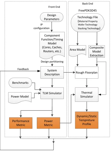
Figure 3.1 System-level CAD flow for 3D design space exploration. . . 33
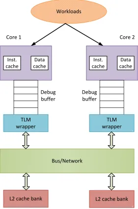
Figure 3.2 Dual-core chip multiprocessor (CMP) system. . . 35
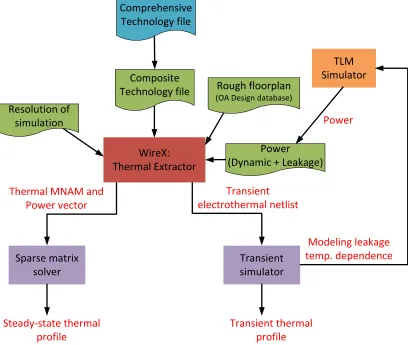
Figure 3.3 System-level electrothermal simulation flow. . . 38
Figure 3.4 Cross section of the first three tiers of the FreePDK3D45 technology. . . . 40
Figure 3.5 Cross section view of unit cell used in parallel-orthogonal conductivity calculation. . . 42
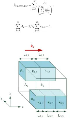
Figure 3.6 Cross section view of unit cell used in orthogonal-parallel conductivity calculation. . . 43
Figure 3.7 Equivalent thermal conductivities obtained using parallel, orthogonal, parallel-orthogonal, and orthogonal-parallel models for various metal den-sities. . . 44
Figure 3.8 Lock-step synchronization mechanism for the electrothermal simulation. . 47
Figure 3.9 Leakage-temperature dependence for one read and one write port SRAM bitcell. . . 49
Figure 3.10 Floorplan of quad-core 2D system considered for the comparison between HotSpot and Pathfinder3D. . . 51
Figure 3.11 Thermal profile of quad-core 2D system obtained using HotSpot. . . 52
Figure 3.12 Thermal profile of quad-core 2D system obtained using Pathfinder3D. . . 52
Figure 3.13 Two floorplans for stacking cores and L2 cache banks of a dual-core CMP system: a) core over core and cache over cache stacking (FLP1), b) cache over core stacking and vice versa (FLP2). . . 53
Figure 3.14 Dynamic thermal profile of core on both tiers with and without consid-ering leakage-temperature positive feedback in core over core and cache over cache stacking (FLP1). . . 55
Figure 3.15 Dynamic thermal profile of core on both tiers with and without consid-ering leakage-temperature positive feedback in cache over core stacking and vice versa (FLP2). . . 56
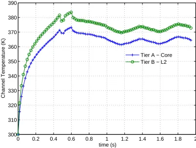
Figure 3.16 Channel temperature of core on Tier A and L2 bank on Tier B of FLP2 after implementing dynamic voltage and frequency scaling as a thermal mitigation technique. . . 57
Figure 3.17 Impact of workload distribution across different tiers in 3D stack on tem-perature. . . 59
Figure 3.18 Impact of microbump density on temperature in 3D stack. . . 60
Figure 3.19 Design space for power modeling. . . 62
Figure 3.21 Flow for statistical transient power model construction and power predic-tion. . . 66 Figure 3.22 Time series decomposition using the Haar wavelet. . . 67 Figure 3.23 Time series reconstruction using a) all wavelet coefficients, b) highest four
wavelet coefficients. . . 69 Figure 3.24 Boxplot representing the percentage root mean square error in transient
switching power prediction using linear regression for different workloads. 72 Figure 3.25 Boxplot representing the percentage root mean square error in transient
switching power prediction using polynomial regression for different work-loads. . . 75 Figure 3.26 Radial basis function network. . . 76 Figure 3.27 Boxplot representing the percentage root mean square error in transient
switching power prediction using radial basis function-based regression for different workloads. . . 78 Figure 3.28 Boxplot representing the percentage error in average power prediction
using radial basis function-based regression for different workloads. . . 79 Figure 3.29 Comparison of the transient temperature profile obtained using the
sim-ulated and predicted power trace. . . 80
Figure 4.1 Flowchart of macromodel-based dynamic electrothermal simulation method-ology. . . 84 Figure 4.2 Two input electrothermal CMOS NOR schematic with various current
components identified. . . 88 Figure 4.3 Dynamic electrothermal characteristics of the two-input NOR gate: (a)
comparison of the electrical transistor-level, electrothermal macromod-eled, and electrothermal transistor-level responses; (b) temperature tran-sients at electrical switching events. . . 92 Figure 4.4 Channel temperature over time. . . 93 Figure 4.5 3D IC: (a) floor plan of the 3D IC chip; and (b) frequency
multiplier-divider chain. . . 98 Figure 4.6 Electrothermal models: (a) frequency multiplier; and (b) frequency
di-vider. . . 99 Figure 4.7 Measured thermal profile of the die showing nine hotspots and their
lo-cation on the layout of 3D IC. . . 100 Figure 4.8 Transient surface temperature profile obtained from measurement and
junction temperature profile obtained from simulation. . . 102 Figure 4.9 Transient junction temperature profiles of hotspots present in each tier
for two substrate thicknesses. . . 103 Figure 4.10 Electrical and electrothermal response at the multiplier-divider interface. 104
Figure 5.1 Delay elements: (a) ideal state-variable-based delay element; and (b) ideal lossless transmission line. . . 112 Figure 5.2 Splitting one delay element, (a), into two subdelay elements, (b), showing
Figure 5.3 Reference terminals: (a) global reference terminal; (b) local reference ter-minal; (c) element reference terter-minal; and (d) depiction of a multiphysics
electrical and thermal network using LRTs. . . 119
Figure 5.4 Flowchart of parallel simulation methodology. . . 122
Figure 5.5 Multithreaded implementation flow. . . 126
Figure 5.6 Hardware architecture of the shared-memory multicore processor used in this work. . . 129
Figure 5.7 Speedup factor, SF across multiple cores with delay factor, DF =10. . . . 131
Figure 5.8 Delay-based partitioning of phase locked loop. . . 136
Figure 5.9 Parallelization overhead across multiple cores with DF of 10. . . 137
Figure 5.10 Speedup factor, SF and parallelization overhead verses delay factor, DF on 8 cores. . . 138
Figure 5.11 Dynamic electrothermal characteristics of the frequency multiplier chain (ckt2): (a) electrical characteristics; (b) channel temperature transients at electrical switching events. . . 141
Figure 5.12 Dynamic electrothermal characteristics of the frequency multiplier chain (ckt2): channel temperature over time. . . 142
Figure 5.13 Transient response for the soliton line (ckt3) on multiple cores. . . 143
Figure 5.14 Transient output of the 20 bit adder (ckt4) on multiple cores. . . 144
Figure 5.15 Transient output of PLL (ckt8) on 2 cores. . . 145
Figure 5.16 Variation in normalized error with number of relaxation iterations. . . 146
Figure A.1 A snippet of Pathfinder3D technology file written for FreePDK3D45 tech-nology. . . 163
Figure A.2 Cross section of the first three tiers of the FreePDK3D45 technology. . . . 164
Figure A.3 A snippet from Pathfinder3D design file. . . 168
Figure A.4 A snippet from Pathfinder3D interface file. . . 170
Chapter 1
Introduction
1.1
Motivation
The limited performance improvement of transistors in ultra-deep-submicron technologies is
making it more difficult to achieve computing performance increases from scaling alone [1].
Transistors are still getting smaller, but their performance is not increasing at a pace consistent
with Moore’s law. Furthermore, migration to advanced process nodes is facing tremendous cost
increases in lithography and patterning integration [2], slow ramp-up in manufacturing yield,
and large variations in the electrical characteristics of MOSFETs. This situation is further
aggravated by the growing complexity of interconnects. The average length of global wires is
determined by chip size and tends to remain fixed as technology scales, but the delay of a unit
length of wire is increasing [3]. Furthermore, the slowdown in supply voltage scaling makes it
more difficult to reduce power consumption. Three dimensional integrated circuits (3D ICs)
address some of these challenges by stacking different ICs vertically [4, 5]. Circuits in different
tiers of a 3D IC can communicate with each other through different types of through-silicon
vias (TSVs), which can largely reduce the total wire length and routing congestion compared
to a conventional 2D implementation. This results in reduced interconnect delay and power
supporting radio frequency (RF) and high performance logic devices) in a monolithic 3D die.
This type of heterogenous integration is a powerful means of reducing delay and power
con-sumption [6, 7]. Furthermore, even within one technology, different generations (for example 45
nm and 32 nm logic CMOS) can be stacked to realize the cost benefit from the better yield of
the mature node [8].
Unfortunately, there are significant thermal challenges associated with 3D ICs. Increased
volumetric density in 3D ICs leads to large heat-fluxes, and the lower thermal conductivities
of the inter-tier and inter-metal dielectrics restrict the heat flow towards the heatsink, making
heat removal a challenging task. Moreover, die thinning reduces the amount of silicon and
in-creases the proportion of oxide and molding materials whose thermal conductivities are lower
than silicon. These trends result in increased on-chip temperature which can adversely affect
performance (by means of mobility degradation), power (by means of exponential increase in
leakage current), reliability (by means of electromigration, time-dependent dielectric
break-down, negative bias temperature instability, etc.), and cost (by means of increased cooling cost)
of packaged 3D ICs. Furthermore, the positive feedback between leakage current and
tempera-ture may lead to thermal runaway which can destroy the chip [9]. Hence, careful thermal design
facilitated by modeling and simulation is essential for successfully designing cost-effective high
performance 3D ICs. Moreover, it is important to address the thermal issues at different levels
of design abstraction, because this provides various opportunities for optimization at different
design costs. For example, a study by LSI Logic shows that power can be reduced by 20%,
10% and 5% by optimizations at register transfer-level (RTL), gate-level, and transistor-level
respectively whereas 80% reduction can be achieved at the electronic system-level (ESL) [10]. At
the system-level, optimizations can be done with less effort compared to register-transfer level
(RTL), gate, and transistor-level abstractions. Optimizations at RTL, gate or transistor-level
require more involved and detailed gate or circuit simulation for identifying the
opportuni-ties. However, analysis at these levels is still required before design sign-off. This give rise the
designers in electrothermal modeling and simulation.
The electrothermal simulation can be of two types: static or steady-state simulation, and
dynamic simulation. Static simulation determines the final temperature to which an IC
con-verges as time tends to infinity. Static simulation can provide a correct estimate of IC
tem-perature only if the power profile does not change with time or the thermal profile converges
well before the power profile starts changing. Dynamic simulation is required to determine
tem-perature when the power profile changes with time (e.g., different phases of a program can
have different power profiles, transient variations in leakage power due to leakage-temperature
positive feedback loop), and when capturing thermally-induced transient variations of
electri-cal characteristics (e.g., transient degradation in frequency due to temperature rise). Dynamic
electrothermal simulation is more computationally expensive than static simulation because it
requires long times for thermal transients to subside. Hence computationally efficient simulation
methodology is critical for such simulation. This work is focused on fast and accurate dynamic
electrothermal modeling and simulation of 3D ICs at system and gate-level.
In recent years ESL design has become increasingly important as it helps manage growing
system complexity by moving design decisions to higher levels of abstraction [11]. At the
system-level, a system can be easily assembled using simple models of hardware components and fast
architectural exploration can be done. This increases designer productivity [12]. However, one
of the biggest challenges of ESL flows is that they often lack physical awareness. With
contin-ually increasing design complexity, and the limitations imposed by manufacturing choices, it is
important for chip architects to understand how physical-level decisions constrain system-level
decisions. For example, in the 3D IC context, the architectural choice of a thermal
manage-ment scheme can be affected by physical details such as the 3D floorplan, bonding method,
TSV/microbump density and material, and package material properties. Hence consideration
of physical-level details in system-level flows has become a necessity. The term commonly used
for this kind of physically aware virtual prototyping and system-level design space exploration
identify thermally bad designs early in design thus reducing development cost and risk.
Further-more, early thermal analysis facilitates the design of robust and cost-effective runtime thermal
management algorithms for handling thermal emergencies.
Once the system-level flow arrives at a thermally efficient design, detailed simulation is
required for accurately estimating the temporal and spatial variations in temperature across
the 3D stack. It is also required for determining the precise locations of hotspots and capturing
the localized variations in the device parameters around the hotspots. Detailed electrothermal
simulations can be performed at transistor and gate-level. Computations in transistor-level
dynamic electrothermal simulations are prohibitly expensive and hence not suitable for the
large scale simulations [13]. Gate-level electrothermal simulation requires electrothermal model
of standard logic gates. This work uses compact electrothermal macromodel of gates developed
in [14]. Gate-level dynamic simulation using electrothermal macromodels is significantly faster
than transistor-level simulation but it is still not sufficiently fast which can allow multiple
iterations of large scale simulations required during the design phase. This work presents a
parallel simulation technique to speedup the gate-level dynamic electrothermal simulation using
parallel computing power of modern multicore processors.
1.2
Original Contribution
The goal of this work is to develop computer-aided design (CAD) flows, methodologies, and
tools for fast and accurate dynamic electrothermal simulation of 3D ICs. It is crucial to perform
electrothermal simulations at different levels of design abstraction. First part of this dissertation
is focused on flows and methodologies to enable dynamic electrothermal simulation at
system-level. Second part is focused on techniques to speedup the gate-level dynamic electrothermal
simulation.
In this work a pathfinding flow that integrates SystemC transaction-level electrical and
physically-aware dynamic thermal simulations is presented. The flow facilitates the study of
Pathfinder3D [15] is developed to deliver the pathfinding flow presented here. The framework
provides an extremely convenient method to pass physical constraints to system architects. It
enables to examine thermal impact of tremendous range of 3D IC manufacturing options such
as choice of wafer and stack technology, stacking schemes, and bonding methods. Furthermore,
a SystemC transaction-level model (TLM) based electrical simulation approach is presented
which allows a user to conveniently explore the impact of using different available architectural
configurations for component intellectual property (IP) blocks in realistic simulation times.
For example, impact of different bus protocols, and cache hierarchies can be studied by just
swapping SystemC modules.
Another original contribution is the development of a parallel transient simulation technique
for multiphysics circuits. This technique is used to speedup the gate-level dynamic
electrother-mal simulation. The technique develops partitions utilizing the inherent delay present within
a circuit and between physical domains (e.g., electrical and thermal). A state-variable-based
circuit delay element is presented which implements the coupling between two spatially or
temporally isolated circuit partitions. A parallel delay-based iterative approach for interfacing
delay-partitioned subcircuits is applied which achieves the reasonable accuracy of non-parallel
circuit simulation if both incorporate the same inter-block delay. The partitioned subcircuits are
distributed to different cores of a shared-memory multicore processor and solved in parallel. A
multithreaded implementation of the methodology using OpenMP [16] is presented. Examples
showing superlinear speedup compared to unpartitioned single core simulation are presented.
The proposed technique can also be used for expediting the transient simulation of digital,
analog, and radio frequency (RF) integrated circuits.
1.3
Organization
Chapter 2 presents a literature review which includes major approaches to electrothermal
sim-ulation and several techniques for thermal modeling and simsim-ulation of 3D ICs. Furthermore,
circuit simulation. An approach to system-level dynamic electrothermal simulation is presented
in Chapter 3. In this chapter, a thermal pathfinding flow is described in detail, and the
appli-cation of proposed flow is illustrated using case studies. It also presents three statistical power
models of an out-of-order superscalar processor, which are intended to be used for thermal
design space exploration. A macromodel-based approach for gate-level dynamic
electrother-mal simulation is presented in Chapter 4. Chapter 5 presents a parallel transient simulation
technique for multiphysics circuits. A detailed description of proposed simulation methodology,
implementation details, and parallelization speedup achieved for a wide variety of circuits are
presented. Chapter 6 concludes this work.
1.4
Publications
1.4.1 Journals
1. Priyadarshi, S., Steer, M. B., Franzon, P. D., and Davis, W. R.: ‘Thermal Pathfinding for
3D ICs: How to get from a Hot Idea to a Cool Product’, submitted to IEEE Design &
Test of Computers.
2. Priyadarshi, S., Saunders, C., Kriplani, N., Demircioglu, H., Davis, W. R., Franzon, P.
D., and Steer, M. B.: ‘Parallel Transient simulation of Multiphysics Circuits Using
Delay-Based partitioning’, IEEE Transactions on Computer-Aided Design of Integrated Circuits
and Systems, Oct. 2012, 31, (10), pp. 1522-1535.
3. Priyadarshi, S., Harris, T. R., Melamed, S., Ortero, C., Manohar, R., Dooley, S. R.,
Kriplani, N. M., Davis, W. R., Franzon, P. D., and Steer, M. B.: ‘Dynamic Electrothermal
Simulation of Three Dimensional Integrated Circuits using Standard Cell Macromodels’,
IET Circuits, Devices and Systems, Jan. 2012, 6, (1), pp. 35-44.
4. Harris, T. R., Priyadarshi, S., Melamed, S., Ortero, C., Manohar, R., Dooley, S. R.,
Analysis of Three-Dimensional Integrated Circuits’, IEEE Transactions on Components,
Packaging and Manufacturing Technology April 2012, 2, (4), pp. 660-667.
5. Melamed, S., Thorolfsson, T., Harris, T. R., Priyadarshi, S., Franzon, P. D., Steer, M.
B., and Davis, W. R.: ‘Junction-Level Thermal Analysis of Three Dimensional Integrated
Circuits using High Definition Power Blurring’, IEEE Transactions on Computer-Aided
Design of Integrated Circuits and Systems, May 2012, 31, (5), pp. 676-689.
6. Schinke, D., Priyadarshi, S., Shepherd Pitts, W., Di Spigna, N., Franzon, P. D.:
‘SPICE-compatible physical model of nanocrystal floating gate devices for circuit simulation’, IET
Circuits, Devices and Systems, Nov. 2011, 5, (6), pp. 477-483.
1.4.2 Conferences
1. Priyadarshi, S., Choudhary, N., Dwiel, B., Upreti, A., Rotenberg, E., Davis, W. R., and
Franzon, P. D.: ‘Hetero2 3D Integration: A Scheme for Optimizing Efficiency/Cost of
Chip Multiprocessors’, Proc. IEEE International Symposium on Quality Electronic Design
(ISQED), March 2013.
2. Franzon, P. D., Priyadarshi, S., Lipa, S., Davis, W. R., and Thorolfsson, T. ‘Exploring
Early Design Tradeoffs in 3DIC’, Proc. IEEE International Symposium on Circuits and
Systems (ISCAS), May 2013.
3. Priyadarshi, S., Hu, J., Choi, W. H., Melamed, S., Chen, X., Davis, W. R., and Franzon,
P. D.: ‘Pathfinder 3D: A Flow for System Level Design Space Exploration’, Proc. IEEE
International 3D System Integration Conference (3DIC), Feb 2012, pp. 1-8.
4. Franzon, P. D., Davis, W. R., Zheng Zhou, Priyadarshi, S., Hogan, M., Karnik, T., and
Srinavas, G.: ‘Coordinating 3D designs: Interface IP, standards or free form ?’, Proc. IEEE
5. Priyadarshi, S., Kriplani, N., Harris, T., and Steer, M. B.: ‘Fast Dynamic Simulation of
VLSI circuits using Reduced Order Compact Macromodels of Standard Cells’, Proc. IEEE
Chapter 2
Literature Review
2.1
Introduction
There are four key design challenges associated to 3D ICs which must be addressed for the
widespread adaptation of this technology. These challenges are associated to a) heat
dissipa-tion, b) power delivery network design, c) floorplanning, and d) design for test. The thermal
issues in 3D ICs affect all other design concerns which makes the modeling of interaction
be-tween electrical and thermal characteristics an absolute necessity than ever before. For example,
increased temperature in 3D stack can magnify the strength of positive feedback loop between
self-heating (i.e. joule heating) in power grid and temperature-dependent electrical resistivity
which can significantly increase the IR drop in the power grid. Furthermore, the positive
feed-back loop between leakage power and temperature strengthened by increased temperature in the
3D stack can significantly change the power density and constrain the floorplanning
optimiza-tions. The thermal induced TSV stress can affect the mobility of transistors in the proximity of
TSVs causing timing variations in 3D ICs which makes the delay-fault testing more challenging.
Several techniques have been previously presented for the thermal modeling and
simula-tion of 3D ICs. However, fewer have explored the electrical-thermal co-simulasimula-tion of 3D ICs.
architecture-level i.e. coarse-grained methods, and b) techniques at the gate or transistor-level
i.e. fine-grained methods based on the level of design abstraction they are exercised.
Further-more each category can have two types of simulation methods namely a) static or steady state,
and b) dynamic or transient simulation. This chapter will first present the basic principle of
electrothermal simulation. Later, research works published around aforementioned categories
and simulation methods are presented.
2.2
Electrothermal Simulation
The time dependent three dimensional heat diffusion equation is
ρc∂T
∂t =Q(x, y, z, t) +k(T)
∂2T ∂x2 +
∂2T ∂y2 +
∂2T ∂z2
(2.1)
whereT is temperature, t is time, ρ is material density,c is specific heat, andQ(x, y, z, t) is
the rate of heat generation and k is temperature dependent thermal conductivity.
Given a boundary condition, the temperature profile can be obtained by solving Eq. 2.1. In
Eq. 2.1, the heat generation rateQ(x, y, z, t) is equivalent to the power consumption in electrical
system. So electrothermal simulation requires close interaction between electrical and thermal
simulations. The electrical simulation is required to obtain information on power dissipation
which is fed to the thermal simulation. The thermal simulation is required to obtain
temper-ature information which is fed to electrical simulation and tempertemper-ature dependent electrical
parameters such as leakage current, mobility, and threshold voltage etc. are updated
accord-ingly. In dynamic electrothermal simulation, there are two approaches to model the coupling
between electrical and thermal simulations namely a) relaxation, and b) direct method.
In the relaxation method, electrical and thermal simulations are performed separately with
temperature updates passed from the thermal simulator to the electrical simulator and power
updates passed from the electrical simulator to the thermal simulator [17, 18, 19]. These
hun-dreds of clock cycles or more for a digital circuit. In transistor-level electrothermal simulation,
SPICE, ELDO, SABER or similar circuit simulator can be used for the electrical simulation.
The thermal simulation can be done using numerical volume meshing techniques discretizing
the differential operators (finite difference method [20, 21]) or the field quality (finite element
method [19]). These numerical techniques are fairly accurate but computationally expensive
due to huge size of equivalent thermal circuit obtained due to volume meshing. The size of
equivalent thermal circuit can be reduced by using model order reduction techniques or by
reducing the mesh density (i.e. coarse grain meshing). Alternatively, analytical techniques such
as Green’s function-based methods [22, 23] can be used. In these methods, Green’s function is
used to describe the temperature response to a unit power source. Then responses from all the
power sources are combined to calculate the full response. These methods are fast but limited
to problems with regular geometry and well-defined usually constant thermal properties. In
the system-level electrothermal simulation, electrical characteristics can be modeled using
Sys-temC transaction-level simulation and numerical techniques with coarse-grain volume meshing
or Green’s function-based analytical methods can be used for thermal simulation.
In the direct method [24, 25, 20, 26], an electrical circuit model of a thermal system is
created based on the thermal-electrical analogies shown in Table 2.1 [27]. The electrical and
thermal circuit models are solved simultaneously as if they were one large electrical circuit
model. This effectively converts an electrothermal simulation to pure electrical simulation.
Table 2.1: Thermal-electrical analogy
Thermal Electrical
TemperatureT[K] VoltageV[V]
Heat,Q[J] Charge,Q[C]
Heat transfer rate,q[W] Current,i[A]
Thermal resistance,RT [K/W] Electrical resistance,R[V/A] Thermal capacitance,CT [J/K] Electrical capacitance, C[C/V]
The heat transfer rate (q) and electrical current (i) are functions of temperature (T) and
voltage (V). The heat transfer rate corresponds to power dissipation in an electrical system.
This method requires solving the following set of equations using iteration [20]:
YE 0 0 YT H
V T =
i(V, T)
q(V, T)
(2.2)
In Eq. 2.2, YE corresponds to the electrical modified nodal admittance matrix and YT H
corre-sponds to thermal admittance matrix.
The relaxation method is easier to implement as existing electrical and thermal simulators
can be directly used but accuracy of this method cannot be assumed in strongly-coupled thermal
problems [24, 25]. Furthermore, very fast changes cannot be considered in this method [20].
The direct method requires a more complex physically-consistent implementation than does
the relaxation approach but is capable of handling very fast changes [28]. In general, for large
scale simulations, relaxation methods are computationally more efficient than direct methods
but direct methods are more accurate than relaxation methods. In relaxation methods, a trade
off between simulation speed and accuracy can be done by changing the length of interval after
which the electrical and thermal simulators exchange their updates. In the work presented in
this dissertation, relaxation method is used for system-level simulation because of its relative
simplicity of implementation and better computational efficiency which is essential for exploring
large design space. The direct method is used for gate-level simulation because of its better
accuracy.
2.3
System or Architecture-level Electrothermal Simulation
In this section architecture-level techniques for thermal simulation are presented. Features and
3D specific limitations of the state-of-art architecture-level thermal simulator HotSpot [29]
are described in detail. Then, the basics of transaction-level modeling are presented. At last,
Puttaswamy et al. performed architecture-level steady state thermal evaluation of high
per-formance microprocessors built using 3D integration [30]. They compared the temperatures of
a 2D, 2-die 3D, and 4-die 3D implementations of Alpha 21364 processor and proposed several
techniques to reduce 3D power density. They used HotSpot [29] tool for thermal simulations.
HotSpot constructs a compact transient thermal model of a microprocessor modeling the heat
transfer path from the silicon die to the ambient. In this model, microarchitectural blocks are
represented by an equivalent circuit of thermal resistances and capacitances. It also allows to
incorporate the cooling aspects of the package in the model. Moreover, it also provides the
flexibility to model the secondary heat transfer path from silicon to C4 pads to packaging
substrate to solder balls and printed-circuit board. HotSpot solves the heat differential
equa-tions describing the RC circuit at each time step using a fourth-order Runge-Kutta method.
HotSpot takes a transient power trace as input for which it typically relies on an external
detailed cycle-accurate performance/power simulator like SimpleScalar/Wattch [31], [32]. The
detailed architectural simulation approach works well if only the processor alone is considered,
but this approach is not feasible for simulation of System-on-chip (SoC) containing several
pro-cessors, memory, bus etc. in realistic simulation times. HotSpot was originally developed for
the architecture-level thermal analysis of 2D ICs and later extended to some extent for 3D ICs.
However, it has several 3D specific limitations. For example, currently it does not explicitly
support modeling of TSVs and microbumps. Their geometry (e.g., thickness, diameter), pitch,
and density can hugely impact the temperature in the 3D stack. For example, Lau et. al. [33]
have shown that for the TSV pitch of 0.2 mm and 0.3 mm, increasing the TSV aspect ratio
(thickness/diameter) from 2 to 4, reduces the equivalent thermal conductivity inzdirection by
30% and 20% respectively. HotSpot tool manual suggests a work around for modeling TSVs
which include manually changing the thermal conductivity (in the source code) of the grid cells
at which the TSVs are located. This approach will work, however, it requires a user to identify
exact grid locations where the TSVs are located which is very time consuming and
this process need to be iterated every time when the TSV density is changed.
Modeling of different 3D bonding methods such as face-to-face, face-to-back, etc. are also
not supported in HotSpot. The bonding style affects the placement of thermal vias and hence
temperature [34]. For predicting the temperature in the 3D stack it is essential to model the 3D
specific physical details. Moreover, it is also necessary to provide a fast and convenient
mech-anism which allows prediction of the thermal properties of a 3D stack from the information in
most technology/design rule manuals. Pathfinder3D eliminates these 3D specific limitations and
proposes a fast approach for generating transient power trace using SystemC TLM simulation.
Another architecture-level technique for fast transient thermal simulation of microprocessors
is reported in [35]. This technique uses the same approach as used in HotSpot for generating
the equivalent RC model from the floorplanning information. However, the transient simulation
method used in this technique differs from the traditional integration-based transient analysis
method used in HotSpot. In this paper, authors have observed a periodic behavior in the power
consumption of architectural blocks of a microprocessor running typical workloads. Exploiting
this observation, authors have divided the power trace into two components namely a) DC
component, and b) periodic component. A fast frequency domain spectral analysis method is
used to calculate the periodic steady-state response of temperature. Furthermore, a moment
matching method is used to calculate the transient temperature response due to initial condition
and DC power input. Thus obtained periodic steady-state and transient responses are added to
obtain total transient response. Authors have claimed that this approach resulted in 10--100×
speedup over the traditional integration-based transient analysis techniques with little accuracy
loss. However, this technique has 3D specific limitations similar to HotSpot.
2.3.1 SystemC Transaction-level Modeling
A fast electrical simulation technique is one of the key ingredients of the system-level
electrother-mal analysis. One way to expedite the electrical simulation is by raising the abstraction-level
Timing
Port/Pin
Untimed
Loosely
Timed
Approx
Timed
Cycle
Accurate
No pin/
port
Sockets
Pin
accurate
Functional /
Instruction set
Microarchitecture /
Pipeline
RTL
TLM
the levels of modeling abstraction. It categorizes the models based on timing and pin
abstrac-tions. At one end, there is a functional or instruction set model which has no notion of timing
and does not contain any information about how data goes in and out of the modules (i.e., no
pin/port details). On the other end, there is RTL model which is cycle and pin accurate. Any
modeling abstraction which has some notion of timing and some notion of pin connections can
be termed as transaction-level model (TLM). SystemC provides specific libraries and templates
for the reference TLM implementation. SystemC is an extension to the C++ language which
provides new classes and application programming interfaces giving the flexibility to model
both hardware and software in an unified environment. SystemC has an event-driven kernel
which allows to model the inherent concurrency of the hardware. Furthermore, it also supports
the hardware specific data types. Hardware can be modeled at various abstraction-levels from
untimed functional-level to cycle-accurate RTL-level.
In transaction-level modeling approach, computation is separated from the communication
in a system and details not required at early phases of the design flow are hidden. This
re-sults in fast simulation. In a TLM representation, IP blocks contain concurrent processes that
execute their behavior while communication is abstracted from cycle-by-cycle operation to
ab-stract transaction operations. Communication mechanisms (e.g., busses, FIFOs) are modeled as
channels which hide the communication protocols from the IP blocks/modules. In the SystemC
implementation of the TLM standard, channels are derived from the SystemC interface class.
This class specifies the methods used to transport the data without implementing the methods.
The channel actually implements the methods specified in the interface class from which it is
derived. A module communicates with a channel by just calling the functions specified in the
interface class. This enables fast design space exploration. For example, a system architect can
explore the different bus protocols by just swapping the channel models implementing those
protocols as long as channel models are derived from the same interface class. Note that a
module can simply switch between the channels without any recoding because it accesses the
In transaction-level modeling approach, focus is more on what data are transferred and
between which locations rather than how data are transferred. Hence, functionality of each
individual hardware signal is not modeled but instead functionality of a collection of signals is
modeled. These attributes make TLM simulations orders of magnitude faster than RTL
simu-lations and thus, suitable for early architecture-level design space exploration, and performance
modeling. Furthermore, TLM models can be available before the RTL implementation
facili-tating early start of software development by enabling software testing on virtual model of the
hardware platform. A TLM model can also act as a golden model for the hardware functional
verification guiding early verification suite development.
TLM 2.0 Standard
SystemC TLM 1.0 was the first effort to raise the the design abstraction to achieve the
afore-mentioned benefits. However, it has two major limitations with respect to the modeling of
memory-mapped buses [36]. The first shortcoming is lack of standard transaction class which
re-sults in poor inter-operability between the TLM models developed by different vendors severely
restricting the IP reuse. The second limitation is lacking support for timing annotation. Hence
models do not have a standard protocol for communicating the timing information. SystemC
TLM 2.0 is an extension of TLM 1.0 which eliminates aforementioned limitations and provides
a new standard for inter-operability between memory-mapped bus models. There are four
fun-damental concepts associated to TLM 2.0 standard namely a) transport interfaces, b) generic
payload, c) sockets, and d) base protocol. SystemC TLM 2.0 supports two types of transport
interfaces. The first being blocking interface using which transport is completed in a single
func-tion call. This interface is only able to model the start and end of a transacfunc-tion. The second
transport method is called nonblocking interface method which allows to break a transaction
into multiple time points and generally requires multiple function calls for a single transaction.
The presence of multiple time points within the execution of a single transaction makes
methods.
Generic payload is a standard transaction class added in TLM 2.0 to improve the
inter-operability of memory-mapped bus models. This class contains several standard parameters
associated to memory-mapped bus protocols including command, address, byte enables, transfer
mechanism (single word or burst transfer), streaming, and response status. Note that the generic
payload class does not include the precise details of the bus protocols. TLM 2.0 introduces the
concepts of initiator, target, and socket to describe the flow of transactions. An initiator is a
module that initiates new transactions, and a target is a module that responds to transactions
initiated by other modules. Objects of the generic payload class are passed between the initiators
and the targets. SystemC ports and exports are connectors through which the payload objects
are passed between the initiators and the targets. A call to a transport interface method is
initiated on a port. Then, a corresponding export which is connected to the port, responds.
TLM socket is a combined port and export. A socket represents a bidirectional connection
between the initiator and the target.
TLM 2.0 defines base protocols to model the time progression. A base protocol is set of
rules associated to sequence of timing phase transition and timing annotations on transport
methods. A TLM transaction can pass through several busses having different protocols (thus
different TLM models). The rules defined in the base protocols facilitate the inter-operability
between different TLM models.
TLM 2.0 Timing Abstractions
SystemC TLM 2.0 [36] standard introduced two timing abstractions namely a) loosely timed
(LT) model, and b) approximately timed (AT) model. A loosely timed model provides timing
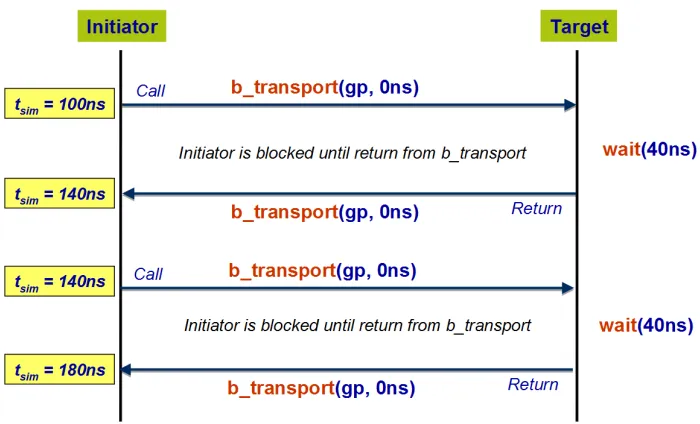
at the granularity of the individual transaction. A loosely timed model typically uses a blocking
interface method, i.e., calling process is halted (using wait()) until the transport is complete.
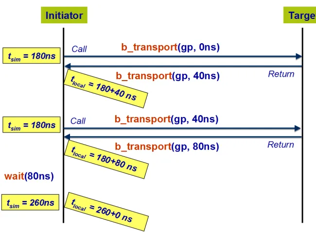
This is illustrated in Figure 2.2 (This image is taken from [37]). TLM 2.0 introduced the concept
different from the global view of simulation time maintained by the SystemC kernel. Using
this concept, a process in loosely timed model can run ahead of the simulation time until it
needs to synchronize with another process. At the synchronization point a wait() statement of
accumulated local time can be inserted to model the latency as shown in Figure 2.3 (This image
is taken from [37]). This results in faster simulation due to fewer context switches. However,
apart from thewait() method call, no explicit mechanism exists for the synchronization. These
models are easier to code as less details are considered in the coding.
Figure 2.2: Blocking transport without temporal decoupling.
An approximately timed model breaks down a transaction into four timing phases namely
a) BEGIN REQ, b) EN D REQ, c) BEGIN RESP, and d) EN D RESP. This requires
multiple function calls to execute a full transaction. These models typically use a nonblocking
interface method which returns a value from the set (T LM ACCEP T ED,T LM U P DAT ED,
T LM COM P LET ED) to indicate the status of the transaction. The timing phases and the
ap-Figure 2.3: Blocking transport with temporal decoupling.
proximately timed models more accurate than loosely timed models. However, AT models are
slower than LT models because in AT models processes run in the lock-step with the simulation
time and several function calls are required to execute a transaction.
2.3.2 System-level Thermal Management
Cooling cost of a chip can be significantly reduced by designing cooling solutions for average
power instead for peak power because peak power and resulting peak temperature is not very
frequently observed. However, this requires dynamic thermal management (DTM) techniques
which restrict any occurrence of such infrequent peak temperature scenarios (also called thermal
emergency). DTM mechanisms allow to achieve better performance compared to pessimistically
designed systems based on the worst case power by detecting and resolving thermal emergencies
either reactively or proactively. Implementation of DTM mechanisms is more complex in 3D
lateral heat flow between the units within the same layer is limited resulting in heterogenous
thermal characteristics across 3D stack. Furthermore, units closer to heat sink cool down faster
than those further away from the heat sink resulting in different cooling efficiency of different
layers [38].
A system-level thermal optimization algorithm for 3D multiprocessor system-on-chip
(MP-SoC) is presented in [39]. It first uses a power balancing algorithm to distribute tasks among
processor cores. Then an iterative hotspot mitigation algorithm is used to reduce the peak
temperature by adjusting the task execution times and voltage levels based on detailed thermal
analysis. In this work the authors also studied the impact of heterogenous thermal characteristics
of 3D MPSoC and heterogenous power characteristics of workloads on thermal optimizations.
Zhu et al. have proposed a runtime thermal management solution, calledT hermOS, for 3D chip
multiprocessors (CMP) [40]. The solution consists of a family of thermal management policies
guiding a proactive continuously engaged hardware-software thermal management scheme. In
this scheme, the hardware facilitates temperature and workload monitoring and software
(op-erating system) dictates power-thermal budgeting and temperature-aware workload migration.
Authors have studied the attributes of existing 2D thermal management techniques such as
dynamic voltage and frequency scaling (DVFS) and workload scheduling etc. for 3D multicore
architectures in [38]. Furthermore, they have also proposed a new dynamic thermally-aware
job scheduling policy called,Adapt3D. This technique considers the cooling efficiency and the
thermal history of each core in balancing the temperature and reducing the frequency of the
hotspots. Their results show that Adapt3Dhas a negligible performance overhead and can be
combined with DVFS to reduce the energy consumption.
2.4
Gate or Transistor-level Electrothermal Simulation
Gate or transistor-level electrothermal simulations are essential for the accurate estimation
of the temperature in the 3D stack before the design sign-off. In this section, first, recently
(both steady-state and transient) of 3D ICs are presented. Later, techniques to speedup the
transient simulation by exploiting the parallel computing power of multicore processors are
presented.
2.4.1 Steady-state Simulation
Park et al. [41] have developed a matrix convolution technique, called Power Blurring for
in-creasing the computational efficiency of the static thermal simulation of 3D ICs. This is a
superposition-based approach where thermal impulse response (also called thermal response
mask) is convolved with power map to determine full-chip thermal profile. The thermal impulse
response is basically thermal profile obtained by applying an unit heat source to the center of
the chip. Thermal measurement or grid-based numerical techniques such as the finite difference
and the finite element methods can be used for calculating the response mask. Temperature of
a tier in the 3D stack is affected by its own power consumption as well as heat transferred from
the other tiers. Thus, temperature profile of a tier is obtained by superposition of temperature
rises due to its own power dissipation and heat transferred from all the other tiers. Hence,
each tier requires a separate thermal mask corresponding to every other tier in the 3D stack.
Melamed et al. [42] have extended the Power Blurring technique to model the 3D chips designed
in silicon-on-insulator (SOI) processes and facilitate the full-chip transistor-level static thermal
simulation of SOI-based 3D ICs in realistic simulation times. They also proposed that thermal
response of a heat source can be divided into a high-fidelity near response and low-fidelity far
response. The near response can be estimated by performing the detailed matrix calculation to
determine the heat flow through a metal-oxide composite material. However, the far response
can be calculated using an average thermal conductivity model for the metal-oxide composite.
Jain et al. [43] have developed a one dimensional analytical heat transfer model for a
multi-layer 3D IC containing multiple heat sources. The proposed resistive model extends the concept
of single-valued junction-to-air thermal resistance into a resistance matrix to capture the impact
rise in theithlayer due to heat dissipation in thejthlayer is modeled using a dedicated thermal resistance,Rij. The thermal resistance matrix include all such resistances. They have also built a numerical model for calculating inter-die thermal resistance which hugely depends upon the
type of inter-die bonding. These models are used to analyze the impact of various geometric
parameters and 3D specific features such as TSV, inter-die bonding, etc. on the steady-state
temperature of 3D ICs.
2.4.2 Transient Simulation
A hierarchial transient electrothermal simulation methodology for large scale 3D ICs which
uses dynamic modeling of the thermal network is reported in [44]. In the first level of the
hierarchial simulation thermal boundary conditions of a small cuboid is determined using the
finite element thermal modeling of the whole chip and the package. Then, within the cuboid,
the electrothermal macromodels (more on this in Chapter 4) [45] of the standard logic gates
are coupled with thermal RC network. In this work, authors have also introduced the concept
of time-scaling to reduce the computational cost of the transient electrothermal simulations.
The time-scaling is implemented by reducing the thermal capacitance and thus thermal time
constant by a factor of ten which reduced the time to reach the steady-state. The scaling factor
should be chosen after a careful study of the tradeoff between the temporal resolution of the
simulation and the computational cost.
A fast and accurate full-chip transient thermal analysis approach for 2D/3D ICs exploiting
the computational throughput of massively parallel graphics processing units (GPUs) in
com-bination with neural networks is reported in [46]. At first, neural network-based thermal model
is developed assuming thermal properties of the materials in IC does not change with
tempera-ture. With this assumption, the system of ordinary differential equations modeling the heat flow
represents a linear time-invariant system for which a linear single layer neural network is
suffi-cient. Usually neural network-based techniques are computationally expensive, however, their
parallelization using GPUs. Thus, the neural network-based thermal simulation is performed
on GPUs which give significant speedups when compared to the conventional techniques.
2.4.3 Parallel Transient Simulation
Transient simulation of very large scale integrated circuits is challenging largely because of
increased simulation times. This situation is further aggravated for specific kinds of transient
simulations, such as multiphysics dynamic electrothermal analysis, which requires long times
for thermal transients to subside. With the advent of multicore technology, low cost large-scale
parallel processors are widely available. The parallel computing power of multicore processors
can help in addressing the computational requirements of transient circuit simulation. However,
efficient exploitation of this requires techniques to partition the circuit for parallelization and
methods to synchronize communication between the circuit partitions. This is because modern
numerical solution of circuit equations represents only a small part of total transient simulation
time.
There are two basic approaches to transient circuit simulation: the direct method and the
relaxation method. The direct method typically uses the following three basic steps [47]: a) time
marching integration methods are used to convert the differential equations into a sequence of
systems of nonlinear algebraic equations; b) a Newton-Raphson method is used to convert the
nonlinear equations into linear equations; and c) the resulting sparse linear equations are solved,
typically using Gaussian elimination or Lower-upper (LU) decomposition. The following
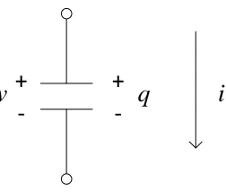
exam-ple illustrates the mathematical formulation of aforementioned steps taking nonlinear capacitor
as a representative example circuit (see Figure 2.4). The mathematical formulation described
below is taken from the lecture material of the course Computer-Aided Circuit Analysis (ECE
718) taught by Dr. Michael B. Steer at North Carolina State University.
Consider the following differential equation representing a nonlinear capacitor
i(t) = dq(v)
+
-v
+
-
q
i
Figure 2.4: A nonlinear capacitor.
whereq(v) is nonlinear function of voltage. This differential equation can be discretized in time
domain using three time marching integration methods namely a) Forward Euler, b) Backward
Euler, and c) Trapezoidal. Backward Euler formula is considered in this example. The Backward
Euler integration method for solving the differential equation
˙x =f(x) (2.4)
is
xn+1 = xn+h˙xn+1 (2.5)
where xn+1and xnare values at timetn+1=tn+h and timetnrespectively. The obvious problem here is how to determine ˙xn+1 when xn+1 is not known. The solution is to iterate as follows: a)
assume some initial value for xn+1 (e.g. using the Forward Euler formula : xn+1 = xn+h˙xn),
and b) now iterate to satisfy the requirement ˙xn+1 =f(xn+1, t).
Using the Backward Euler formula of Eq. 2.5 in discretizing the Eq. 2.3 leads to the following
form of the constitutive relation
in+1=
1
h(qn+1−qn) (2.6)
functionality modeled asi=f(v) is given by
j+1i=f(jv) +δf(jv)
δjv
h
(j+1)v−jvi (2.7)
Using the Newton-Raphson iteration formula of Eq. 2.7, qn+1 is evaluated through the
iteration defined by
(j+1)q
n+1=jqn+1+C(jvn+1)
(j+1)v
n+1−jvn+1
(2.8)
where
C(jvn+1) =
δjqn+1 δjv
n+1
(2.9)
Combining Eq. 2.6 and Eq. 2.8
(j+1)i
n+1=
1
h h
jq
n+1+C(jvn+1)
(j+1)v
n+1−jvn+1
−q(vn)
i
(2.10)
and rearranging
(j+1)i
n+1 =
1
hC(
jv
n+1)(j+1)vn+1+
1
h j
qn+1−q(vn)−C(jvn+1)jvn+1
(2.11)
Note that Eq. 2.11 is a linear equation resulted from applying the Newton-Raphson iteration.
A circuit consisting of several elements will have several such equations and together they form
a system of linear equations which can be solved using Gaussian elimination or Lower-upper
(LU) decomposition.
In the context of three basic steps associated to direct method, the simulation time of the
direct method has three major components: a) model evaluation — involving linearization of
nonlinear device characteristics and Jacobian matrix calculation; b) matrix build — involving
construction of a sparse matrix equation in the formAx=b; and c) matrix solve — the solution
Various techniques have been explored to parallelize device model evaluation and matrix
solve in direct methods using fine-grain parallelism [48, 49]. These fine-grained techniques can
speedup simulation, but speedup due to these techniques may stagnate once the number of
pro-cessor cores reaches a certain point [50]. Alternatively, relaxation approaches to parallel
tran-sient circuit simulation are iterative methods and include Waveform Relaxation (WR-operating
at the nonlinear differential equation level) [51, 52, 53] and Nonlinear Relaxation (operating at
the nonlinear algebraic equation level) [54, 55] methods. However, the speedup from parallelism
of these methods is sensitive to the partitioning algorithm and conditions required for rapid
and stable convergence.
Recently the WavePipe [56], MAPS [57] and HMAPS [50] parallelization techniques were
proposed for multicore shared-memory machines. WavePipe exploits coarse-grained
application-level parallelism by simultaneously computing circuit solutions at multiple adjacent points in a
circuit. MAPS explores inter-algorithm parallelism by starting multiple simulation algorithms
in parallel for a given task. HMAPS adds fine-grained intra-algorithm parallelism to the
coarse-grained inter-algorithm parallelism offered by MAPS [57]. TITAN [58] and Xyce [59] are
SPICE-type parallel circuit simulators which use complex circuit partitioning algorithms to achieve
well-balanced partitions and minimal communication cost among the processors. TITAN partitions
the circuit by minimizing the total wire length for the circuit. Xyce uses weighted graphs and
leading-edge graph decomposition heuristics to partition the circuit graph. These simulators are
well suited to distributed memory multiprocessor systems i.e. computer clusters. The technique
in [60] proposes an overlapping domain decomposition approach to partition the circuit into a
linear subdomain and multiple nonlinear subdomains based on circuit nonlinearity and
connec-tivity. The linear subdomain and nonlinear subdomains are individually solved in parallel. The
author in [61] presents a spatial parallel architecture for accelerating the SPICE-like simulators
using an FPGA. The hybrid parallel architecture spatially implements the heterogenous forms
of parallelism (model evaluation, sparse matrix solve, and iteration control) available in SPICE.
and between physical domains to partition a multi-domain circuit with each partition simulated
on a different core of a shared-memory machine. A delay element interfacing partitions is used to
formulate the whole domain simulation. Single domain circuit partitioning was also used in the
Mimic Transmission Method (MTM) [62]. MTM maps the transmission delay of interconnects
between subcircuits to the communication digital data link between processors. This circuit
partitioning technique is similar to the technique proposed in this dissertation, but it is targeted
to distributed computer clusters and does not exploit the advantages offered by current
shared-memory multicore processors such as low inter-core communication overhead and increased
cache space utilization. Furthermore, there are no details about the synchronization scheme,
parallelization overhead, and speedup due to parallelization. The proposed technique provides
orthogonal improvements over methods like Wavepipe [56], MAPS [57] and HMAPS [50] and
so can be used in conjunction with these techniques to further speedup simulation.
2.5
Summary
In this chapter the necessity for coupled electrical-thermal (i.e. electrothermal) simulation for 3D
ICs is discussed. The two major approaches to electrothermal simulation namely a) relaxation
method, and b) direct method published in the literature are described. This chapter categorizes
the electrothermal simulation in two groups based on the level of design abstraction they are
performed. The first category is system or architecture-level electrothermal simulation. The
features and 3D specific limitations of state-of-art architecture-level thermal simulator, HotSpot,
are discussed. Fundamentals of transaction-level modeling approach are presented. The basic
concepts presented here are used in describing the system-level electrothermal simulation flow
proposed in the Chapter 3. State-of-art system-level runtime thermal management techniques
for 3D ICs are also reviewed.
The second category of electrothermal simulation discussed in this chapter is performed
at gate or transistor-level. Techniques recently published for the gate or transistor-level static
are reviewed. Techniques for reducing the computational cost of transient simulation using the
parallel computing power of multicore processors are discussed. Furthermore, the parallelization
technique presented in this dissertation is distinguished from the methods published in the