Region of Attraction Estimation of Biological Continuous Boolean Models.

(1)

ABSTRACT

MATTHEWS, MEGAN LEIGH. Region of Attraction Estimation of Biological Continuous Boolean Models. (Under the direction of Cranos M. Williams.)

Quantitative analysis of biological systems has become an increasingly important

re-search field as scientists look to solve current day health and environmental problems.

The development of modeling and model analysis approaches that are specifically geared

toward biological processes is a rapidly growing research area. Continuous approximations

of Boolean models, for example, have been identified as a viable method for modeling

such systems. This is because they are capable of generating dynamic models of

bio-chemical pathways using inferred dependency relationships between components. The

resulting nonlinear equations and therefore nonlinear dynamics, however, can present a

challenge for most system analysis approaches such as region of attraction (ROA)

esti-mation. Knowledge of the ROA for metabolic steady states in plants can give valuable

insight into the robustness and sustainability of favorable phenotypes. This could lead to

more efficient production of biofuels from plant biomass, sustained resistance of plants to

climate change, and growth of agriculture on marginal lands. Continued progress in the

area of biosystems modeling will require that computational techniques used to analyze

simple nonlinear systems can still be applied to nonlinear equations typically used to

model the dynamics associated with biological processes. In this thesis, we assess the

applicability of a state of the art ROA estimation technique based on interval arithmetic

to a subnetwork of the Rb-E2F signaling pathway modeled using continuous Boolean

functions. We show that this method can successfully be used to provide an estimate of

the ROA for dynamic models described using Hillcube continuous Boolean

(2)

(3)

(4)

Region of Attraction Estimation of Biological Continuous Boolean Models

by

Megan Leigh Matthews

A thesis submitted to the Graduate Faculty of North Carolina State University

in partial fulfillment of the requirements for the Degree of

Master of Science

Electrical Engineering

Raleigh, North Carolina

2012

APPROVED BY:

Brian L. Hughes Edward Grant

(5)

DEDICATION

(6)

BIOGRAPHY

Megan Leigh Matthews was born in Greensboro, North Carolina on July 14, 1989. While

growing up she lived in Asheboro, NC, Rowlands Gill, UK, and finally Avon Lake, Ohio

where she spent most of her childhood. In 2007, Megan graduated from Avon Lake

High School in 2007, and then immediately fled the cold to attend North Carolina State

University. After many great experiences including a 5 week study abroad trip in Egypt

and a summer internship in Stuttgart, Germany, she graduated Summa Cum Laude with

Bachelors of Science in Electrical Engineering and a Minor in Middle East Studies in

May 2011. She began research in the field of Systems Biology that summer joining the

(7)

ACKNOWLEDGEMENTS

I would like to thank my advisor Dr. Williams for his excellent guidance and patience

in helping me develop my research. I thank my family and friends for their constant

(8)

LIST OF TABLES

Table 2.1 Boolean State Table . . . 12

Table 4.1 The area of the ROA estimate when the given P matrix is rotated about the equilibrium point . . . 43 Table 4.2 The ROA Estimate with the largest area from Table 4.1 (θ = 15◦)

(11)

LIST OF FIGURES

Figure 2.1 Dependence of reaction ratev, d[P]_dt , on substrate concentration S in Michaelis-Menten kinetics. Vmaxdenotes the maximal reaction rate

that can be reached for a large substrate concentration.Km is the

substrate concentration that results in a half maximal reaction rate. For low substrate concentrations, v increases almost linearly with S, while for high substrate concentrationsv is almost independent of S [21]. . . 11 Figure 2.2 Sample Boolean Network: A activates C and B inhibits C, C=A&!B 11 Figure 2.3 Interval extensions [f]([x]) and [f]∗([x]) (minimal) [19] . . . 16 Figure 2.4 Lyapunov ROA estimate example [26] . . . 18 Figure 2.5 This figure illustrates how initial conditions in the ˙V(x)>0 space

can be contained in the actual ROA despite their trajectories not being contained in the Lyapunov function. . . 19

Figure 3.1 Interval Analysis Approach . . . 24 Figure 3.2 ROA Estimation Algorithm . . . 25 Figure 3.3 Schematic depiction of the simplified Cdc2-cyclin B/Wee1 mutually

inhibitory system [3] . . . 28 Figure 3.4 The Rb-E2F network [50]: (a) Detailed Rb-E2F signaling network

that controls the G1/S transition of mammalian cell cycle. Gray-shaded ovals indicate overlapping or intermediate signaling activi-ties to be lumped. Circled numbers indicate indexes of the regula-tory links. (b) A simplified Rb-E2F network. (c) Robust minimal model for resettable bistability. . . 29 Figure 3.5 . . . 33 Figure 3.6 Finding a quadratic Lyapunov function that gives a larger ROA

(12)

Figure 4.1 The simplified Cdc2-cyclin B/Wee1 mutually inhibitory system: (a) Phase portrait of system. Gray curve→V˙ = 0, Shaded gray area→

V ≤ c∗. Gray point is the saddle points, and the two black points are the stable points. (b) Several level sets of V(x). a a a . . . 38 Figure 4.2 Trajectories of the system. Solid Black→analyzed stable point,

Dashed Black→other stable pt. Gray dot=saddle point . . . 39 Figure 4.3 The original ROA estimate (blue) from section 4.1 and the largest

level sets at three additional orientations of the Lyapunov function around the equilibrium point. The dashed curves mark ˙V = 0 for each of the associated V curves. . . 42 Figure 4.4 Three different ROA estimates oriented at θ = 15◦. The dashed

curves mark ˙V = 0 for each of the associatedV curves. . . 44 Figure 4.5 The actual ROA of the bistable two state system is the area below

the stable manifold (bright green) of the saddle point; compared with the original estimate (blue) and the larger estimate after ro-tation and scaling (purple). The phase portrait was plotted using PPlane [32]. . . 45

(13)

Chapter 1 Introduction

1.1 Overview

Understanding the individual components and the overall dynamic mechanisms

associ-ated with biological processes can have promising implications on biofuel production and

disease control [5][30]. This understanding cannot be attained through the piecewise

qual-itative analysis that has traditionally been used to understand biological processes. For

this reason, mathematical and computational tools are being developed to quantitatively

characterize these systems [20][47]. Biological systems theory is said to be analogous

to power and control systems theory. The goal is to apply the analysis and

computa-tional tools used to evaluate control systems to models of biological processes. Currently,

however, the mechanisms and dynamic interactions in most biological systems remain

unknown. The pursuit of effective approaches for modeling the dynamics of biological

systems along with computational tools that are capable of characterizing the possible

range of model activity remains an open research area.

(14)

Michaelis-Menton kinetics [14], S-systems, General Mass Action (GMA) systems, and the power

law approach [22]. Of these methods, mass action law and Michaelis-Menten kinetics

have been prevalent in the literature [44][33]. These methods, however, require a-priori

knowledge of the kinetics associated with the interactions of the system components.

This knowledge remains unknown for many biological networks and pathways of

practi-cal interest. One approach commonly used to circumvent this lack of knowledge is the use

of Boolean models to describe the interactions of components in biochemical processes.

Boolean models are discrete models that describe observed dependencies or influences

be-tween components, often leaving out detailed kinetics of the interactions [47]. Although

these models are a simplification of the process, they have been shown to reproduce the

qualitative behavior of a biological process [13][15]. Boolean models in their native form,

however, cannot be used to explain or predict the outcome of biological experiments that

yield continuous temporal data. This is because they cannot describe continuous

con-centration levels that change over time. The Hillcube transformation is one method of

transforming Boolean models into continuous models that produce continuous dynamics,

which can be quantitatively compared to experimental data [47]. This approach has been

used to model a variety of biological processes including the spatial gene expression

pat-terns at the murine mid-hindbrain boundary (MHB) to explain the stable maintenance

of the MHB [48].

The canonical form of continuous Boolean representations yield a system of equations

that gives us the ability to use known computational tools to analyze their characteristics.

One such important characteristic of nonlinear systems that is important for biological

systems is the region of attraction (ROA) of an equilibrium point. The region of

attrac-tion is the set of initial condiattrac-tions in a system whose trajectories converge to a stable

(15)

the range of concentrations that will determine if a biological system takes on a certain

set of steady state concentrations, often corresponding to a preferred phenotype.

Knowl-edge of the ROA for an equilibrium point could provide knowlKnowl-edge of the sensitivity of

a biological system to changes in its environment. It can also be used to determine what

perturbations may cause the system to transition to a new phenotype or structure.

For simple 2-dimensional systems, regions of attraction can be easily seen from plots

of phase portraits [37]. For higher dimensions, however, it is difficult to impossible to

intuitively determine the ROA for a given steady state. For this reason, there has been

significant research performed in the last couple decades focusing on methods to

quan-titatively estimate the ROA for nonlinear systems [18][45]. ROA estimation methods for

polynomial models have dominated the literature, with many of these methods using

Lyapunov functions to define the region. A common method for determining a Lyapunov

function involves linearizing the system and then using Linear Matrix Inequalities (LMIs)

to find the coefficients of the functions [7][39]. Various methods have been proposed

to find the largest ROA for a given Lyapunov function, which include sums-of-squares

programming [41], polytopic regions [27], and neural networks [16]. Chesi and Tibken

presented an approach for increasing the accuracy of ROA estimates using the union of

several Lyapunov functions [11][40]. Unlike the models used in many of these approaches,

many biological models are non-polynomial systems [47]. Few ROA estimation techniques

have been proposed for non-polynomial nonlinear systems but uncertainty still remains

about the general applicability of these approaches to a broader realm of nonlinear

mod-els [8][45]. Thus, it is important to assess whether such approaches can be successfully

applied to mathematical structures often used to model biological systems, specifically

(16)

1.2 Motivation

The goal of this work is to develop and implement ROA estimation techniques for

non-polynomial models that are frequently used to model large biological systems. The

ap-proach we develop specifically address the conservativeness of current apap-proaches in the

literature. Our long term goal is to develop an approach that can be applied to assess

the robustness and sustainability of phenotypes in plant systems, and their sustainability

under stressful environmental conditions such as climate change.

1.3 Contributions of this Work

1.3.1 Intellectual Merit

In this document, we present results that affirmatively show that the ROA estimation

approach presented in [45] can be successfully applied to biochemical systems modeled

using continuous Hillcube approximations. We explore the potential limitations of this

ROA estimation technique on this class of nonlinear systems and assess the quality of the

resulting ROA estimate. We also identify a method that selects from an infinite number

of quadratic Lyapunov functions one that could provide an improved estimate of the

ROA to decrease the conservativeness of the current ROA estimation algorithms.

1.3.2 Broader Impacts

The research developed in this thesis is applicable to areas of environmental concern

ranging from developing cleaner fuel derived from sustainable and renewable resources

to international food stability. The ROA estimation techniques described in this

(17)

systems, such as biochemical compounds formed by plants. Our goal is to use ROA

es-timation to determine the robustness of biological systems under environmental stress.

This information can then be used to develop methods to combat the changes that are

begin caused and to preserve dwindling ecosystems.

Trees as a Sustainable Biofuel Source

On-going research in ROA estimation will provide the mathematical foundation for

as-sessing steady state phenotypes of models of lignin biosynthesis. Through this we will

be able to assess the ROA of favorable lignin structures that improve the efficiency of

biofuel production for plant biomass. Understanding how changes in the ROA of lignin

in P. trichocarpa in response to environmental stressors will enhance our ability to use

variations of North American pine trees as sustainable sources of biofuel. The genus

Populus is composed of 25 to 35 species of deciduous plants, including poplar, aspen,

and cottonwood trees, that are native to the Northern Hemishpere. Hybrid poplars are

among the fastest growing hardwood trees in North America, growing 3-5 feet every year,

and can be designed to yield desirable traits for applications such as biofuels production

[35][38]. Hybrid poplars, commonly classified as short-rotation woody crops can be grown

on forestlands or on economically marginal croplands [35]. The high cellulose and

moder-ate hemicellulose and lignin content in poplar trees make them a desirable source for the

production of biofuel. Additionally, poplar wood has lower sulfur content when compared

to switchgrass, which is advantageous in terms of the strict environmental regulations

limiting the sulfur content of transportation fields [35].

Sustainability of Global Food Sources

(18)

global food sources by providing the computational framework needed to understand

how changes in the environment impact plant systems such as commodity crops.

En-vironmental stress factors such as drought, elevated temperature, salinity and elevated

CO2 concentration affect the robustness of plants and pose an increasing threat to the

sustainability of agriculture in the presence of significant global population growth [1].

Plants are evolving to cope with these climate changes, but we are generally unable to

predict how well plants are adapting to these challenges. Insight into how plants are

adapting are important to breeding programs that produce transgenic varieties of crops

with an enhanced tolerance to environmental stress factors.

1.4 Organization

In chapter 2 we discuss a brief background of modeling biochemical systems including the

law of mass action, Michaelis-Menten kinetics, and Boolean modeling. We also provide

an explanation of some of the mathematical techniques used, including interval

arith-metic and linear matrix inequalities. We then provide an outline of the advantages and

disadvantages of current approaches for estimating regions of attraction using the

Lya-punov stability theorem relates to that. Finally, we describe the interval analysis ROA

estimation approach presented by [45] that we utilized in this research.

Chapter 3 sets up the interval analysis ROA estimation technique for a two and three

dimensional biochemical pathway modeled using Hillcube continuous Boolean

approxi-mations. We then discuss the methodology of a proposed algorithm that would identify

a Lyapunov function from the many possible ones to improve the estimate of the ROA.

In Chapter 4 we present and discuss the results of the ROA estimation algorithm

(19)

proposed technique to determine an alternative quadratic Lyapunov function.

Chapter 5 presents ideas for further research in developing ROA estimation algorithms

for the purpose of determining the robustness of plant systems under environmental

(20)

Chapter 2 Background

In this chapter, we present background information on the techniques used in this

docu-ment. Section 2.1 presents a brief background on some of the common system modeling

techniques used, followed by a basic overview of the mathematical techniques used in

section 2.2. Finally, we will go into an overview of regions of attraction and give details

on the previous research that has been conducted in this area in section 2.3.

2.1 Modeling Biological Pathways

2.1.1 Mass Action Kinetics

The Law of Mass Action was introduced in the late 19th century by Guldberg and Waage

as a method of mathematically describing and predicting reaction rates in biochemical

systems. The law states that the rate of change of a substance is proportional to its

concentration. Equation (2.1) describes a simple enzyme conversion from substrate to

product. This reaction comprises of a reversible formation of an enzyme-substrate

(21)

product, P, from the enzyme E. The mass action rate equations are shown in (2.2), where

ki is the respective rate, or kinetic, constant associated with the reactions. These rate

equations show how the concentration of each of the substances changes over time, and

can be used to predict the outcome of the reaction depending on the initial concentration

levels [21].

[E] + [S]k1

k−1 [ES] *

k2 _{[E] + [P]} _(2.1)

d[S]

dt = k−1[ES]−k1[E][S] d[E]

dt = k−1[ES] +k2[ES]−k1[E][S] (2.2) d[ES]

dt = k1[E][S]−(k−1 +k2)[ES] d[P]

dt = k2[ES]

Mass action ODEs can easily become cumbersome and difficult to solve. In the early

20th century Michaelis and Menten found a method of simplifying the mass action kinetics

using assumptions of quasi-equilibrium.

2.1.2 Michaelis-Menten Kinetics

Michaelis-Menten kinetics can be used to simplify mass action ODEs, however, several

assumptions must be made [21]. For the system of ODEs in (2.2), we must assume that

the association and disassociation rates of E and S are much faster than the conversion of

ES to P, in other words, k1, k−1 k2. Additionally if we assume that the initial amount

(22)

The system of ODEs in (2.2) are then expressed as:

d[S]

dt = −

Vmax[S]

km+ [S]

(2.3)

d[P] dt =

Vmax[S]

Km+ [S]

where,

Km =

k−1+k2

k1

Vmax=k2[E]_total [E]_total = [E] + [ES].

Vmax represents the maximum rate, and Km is the Michaelis constant. Km is the

concentration of S that results in a rate v that is equal to half of the maximum rate Vmax. Figure 2.1 illustrates these relationships. By using Michaelis Menten kinetics, the

number of rate equations has been reduced from four, (2.2), to two, (2.3), and the number

of parameters has decreased from three to two [21].

Modeling systems using mass action kinetics or Michaelis Menten kinetics can take

a long time and requires knowledge of the detailed chemical reactions as shown in (2.1).

When these reactions become more complex, as is the case with different levels on

inhi-bitions, the Michaelis-Menten equations are derived again and the functional form of the

equation changes. Problems occur, however, when only interactions are known but the

de-tail chemical reactions are unknown. In these cases, researchers began looking at Boolean

modeling for a faster way to model biological systems with less a priori information.

2.1.3 Boolean Modeling

For cases where only the interactions are known, simpler models have been shown to

(23)

Figure 2.1: Dependence of reaction ratev, d[P]_dt , on substrate concentration S in Michaelis-Menten kinetics. Vmaxdenotes the maximal reaction rate that can be reached for a large

substrate concentration.Km is the substrate concentration that results in a half maximal

reaction rate. For low substrate concentrations, v increases almost linearly with S, while for high substrate concentrations v is almost independent of S [21].

(24)

with binary states where each gene, protein, etc. is either considered to be on (1) or off

(0). These models have been used to predict specific cell sequence patterns of protein and

gene activity as observed in living cells with significantly fewer parameters [13].

Figure 2.2 shows a simple Boolean model example. Here, gene A activates gene C and

gene B inhibits gene C. Logically, this is represented as

C = A&!B (2.4)

where & is the AND function and ! is the NOT function. This means that C is only

activated (1) when A is active (1) AND B is inactive (0). Table 2.1 is the state table for

this interaction.

Table 2.1: Boolean State Table

A B C

0 0 0

0 1 0

1 0 1

1 1 0

Boolean models have been applied to the cell-cycle networks of S. cerevisiae [24],

the mammalian cell-cycle [15], gene regulatory networks determining embryonic

segmen-tation in D. melanogaster [2], and the fission yeast S. Pombe cell cycle [13]. In [13],

Davidich and Bornholdt compared the Boolean model ofS. Pombe they created with an

existing ODE model of fission yeast [43]. Their Boolean model was able to reproduce the

(25)

model required the use of 47 fewer kinetic parameters than were necessary for the ODE

approach.

The main benefit of Boolean models is that they require less knowledge about the

detailed kinetics of the interactions of a system. This allows Boolean models to be created

much quicker and easier than their ODE counterparts. However, discrete models are not

able to describe continuous concentration levels that change over time. This prevents

pure Boolean models from being used to explain or predict the outcome of biological

experiments that yield quantitative temporal data. Continuous Boolean modeling was

developed to combine the comparative ease of Boolean modeling with the ability to

pro-duce continuous dynamics that are often needed to evaluate the stability characteristics

of biological systems.

Continuous Boolean Modeling

There are several different transformation techniques for creating continuous Boolean

models including BooleCubes, min-max and product-sum fuzzy logic, and HillCubes.

BooleCubes are created using multivariate polynomial interpolation and HillCubes are

obtained by applying Hill functions to BoolCubes. Due to their smooth analytical

proper-ties and the accuracy of their transformation, we explored the continuous Boolean model

obtained using the HillCube transformation [47]. HillCube transformations are based on

the assumption that molecular interactions typically show a switch-like behavior. This

response is modeled using sigmoid shaped Hill functions,

f(¯x) = x¯

n

τ(¯xn₊_kn₎. (2.5)

(26)

’on’, and n determines the slope of the curve and is a measure of the cooperativity of the interaction [47]. τ represents the life-time of the species. Continuous Boolean models confine the system dynamics over the range x ∈ [0,1] given that the Boolean representations confine the component values to either 0 or 1.

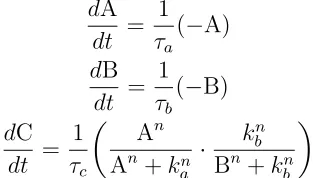
Equation (2.6) uses the HillCube transformation to describe the Boolean model in

Figure 2.2.

dA dt =

1 τa

(−A) dB

dt = 1 τb

(−B) (2.6)

dC dt = 1 τc An An+kn

a

· k

n b

Bn+kn b

Here we can see that that an AND function in the Boolean model is represented as

multiplication, and when one state activates another, the HillCube expression is:

An An+kn

a

. (2.7)

When one state inhibits another the HillCube expression is:

1− B

n

Bn+kn b

= k

n b

Bn+kn b

(27)

2.2 Interval Arithmetic

Interval arithmetic is commonly used as an approach for bounding measurements and

rounding errors in mathematical computation. Typically, arithmetic is used to solve for

exact single point solutions. Interval arithmetic, however, computes the upper and lower

bounds of a solution. It can provide guaranteed solutions by providing solution sets

that include any variation that could be associated with finite arithmetic and round off

error. Interval arithmetic is also valuable in the physical and life sciences due to limited

accuracy in experimental data measurement [29]. Interval extensions of functions are

used when applying interval analysis to traditional arithmetic equations. The interval

extension [f]([x]) of a function f(x) bounds the range of the functionf(x) over the range [x] = [x, x], wherexis the minimum value of the interval and xis the maximum value of the interval. The interval extension of a function provides a result that guarantees that

the true solution is contained in the range. In other words, it guarantees that the interval

[f]([x]) contains all values of f(·) evaluated at all points over the interval [x]. Figure 2.3 illustrates the interval extension of a function. Steps are often taken to ensure that

[f]([x]) is as close to the true solution set, with as little overestimation as possible [28]. Forn-dimensional systems, these intervals, [x] = [x1, x1]×. . .×[xn, xn], form hypercubes

where the minimum and maximum values of the intervals, (xi, xi), form the vertices of

the hypercube.

Interval arithmetic has been used to achieve numerical certification of the kinematic

calibration of a parallel robots [12], reliably calculate phase stability and equilibrium in

industrial processes [36], global optimization of molecular structures [25], to verify the

existence of the Lorenz attractor [42], and to estimate regions of attraction [45].

(28)

Figure 2.3: Interval extensions [f]([x]) and [f]∗([x]) (minimal) [19]

tightness of the enclosure obtained. For example, if the bounded solution is

x∈[0.66666, 0.66667], then the solution, x, is known to 4 decimal places [29].

2.3 Estimating Regions of Attraction

2.3.1 Lyapunov Functions

Lyapunov functions are frequently used to estimate ROAs. Lyapunov functions are used

to define a region around a stable equilibrium point where a trajectory will stay in that

region once entering it. The following Lyapunov Stability Theorem states how knowledge

of this region can be used to provide an estimate of the ROA.

Lyapunov’s Stability Theorem:

For a system containing n states, the closed set Ωc ⊆ ROA, Ωc ∈ Rn×1, is an estimate

(29)

that:

1. V(x) is positive definite on Ωc

2. ˙V(x) is negative definite ∀x6= 0 on Ωc and,

3. ˙V(x) = 0 whenx= 0

The bounded ROA estimate is then:

Ωc :={x|V(x)< c}. (2.9)

This means that once any trajectory enter the region Ωc that trajectory stays inside the

region.

Figure 2.4 illustrates how some level sets of a Lyapunov function are considered

estimates of the ROA and others are not. In this image, Ω1 and Ω2 are both ROA

estimates. Ω2, however, is the better estimate since it is the larger of the two. The largest

level set that can be considered and estimate of the ROA is the set that is tangent to

the curve or surface ˙V(x) = 0 but remains entirely in the space ˙V(x)<0. Ω3 is not an

estimate of the ROA, because even though it is tangent to ˙V(x) = 0 at one location, it crosses into the space ˙V(x)>0. The trajectories of the initial conditions that lie in the space ˙V(x) > 0 exit region Ω3. In order for a region to be considered Lyapunov stable

no trajectory can leave the region. Therefore, Ω3 is not a valid estimate of the ROA.

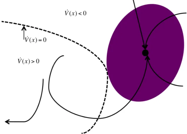
It should be noted that just because an initial condition lies in the ˙V(x) > 0 space does not imply it is not part of the ROA. It is not uncommon for there to be trajectories

that are part of the ROA but are not contained in a quadratic Lyapunov function. It is

(30)

(31)

˙

V(x)>0 space eventually do converge to the equilibrium point and which initial condi-tions have the trajectories that go elsewhere. Figure 2.5 illustrates this characteristic.

Figure 2.5: This figure illustrates how initial conditions in the ˙V(x) > 0 space can be contained in the actual ROA despite their trajectories not being contained in the Lyapunov function.

Most nonlinear systems, including most models of biological processes, can be

ex-pressed as a system of nonlinear differential equations

˙

x=f(x) =Ax+F(x) (2.10)

whereAis the linearization around the equilibrium point andF(x) is a nonlinear function representing the higher order nonlinearities of the process. Lyapunov functions are

(32)

equilib-rium point. While higher order Lyapunov functions potentially provide more accurate

estimates, they are significantly more difficult to compute [11]. A quadratic Lyapunov

function is defined as:

V(x) = xTPx. (2.11)

The time derivative of the Lyapunov function for the nonlinear system in (2.11) is

cal-culated as

˙

V(x) = xT(ATP +P A)x+ 2xTP F(x). (2.12)

The Lyapunov matrix P can be found using computational programs such as MATLAB [17] to solve the following linear constraints:

P =PT >0 ATP +P A <0. (2.13)

2.3.2 ROA Estimation for Nonlinear Polynomial Functions

In this section we describe several different ROA estimation techniques for polynomial

systems that have been presented in the literature.

Research in region of attraction estimation became popular in the mid-80’s.

Gene-sio, Tartaglia, and Vicino’s outlined the, at that time, state of the art and new ROA

estimation proposals in [18]. The methods published in this paper formed the basis for

todays state of the art and new ROA estimation techniques. [18] splits the ROA

esti-mation methods into two main groups, Lyapunov and non-Lyapunov methods. Since the

mid-80’s, the majority of research in ROA estimation has made use of Lyapunov

meth-ods. It became especially prevalent in the late-90s/early 2000’s, when it was determined

that linear matrix inequalities could be used to solve for Lyapunov functions. Below is a

(33)

Graziano Chesi has written several articles on estimating regions of attraction of

non-linear systems using Lyapunov functions and non-linear matrix inequalities (LMIs) [7][6][11][8][9][10].

In [11], Chesi proposes using the union of continuous families of Lyapunov estimates to

approximate the region of attraction. By calculating a parameter-dependent lower bound

using an Eigenvalue problem, a family of estimates of the ROA and the estimate given

by their union can be defined. The advantage of the proposed approach is to provide a

continuous family of estimates rather than one estimate as in existing methods. A

dis-advantage, however, is the larger computational burden in the LMI optimizations which

currently limit the use of the proposed method to low order systems and low degree

Lyapunov functions. Additionally, this method is limited to continuous-time polynomial

systems.

Valmorbida, Tarbouriech, and Garcia propose a method that calculates an ROA

esti-mate for nonlinear polynomial systems using quadratic Lyapunov functions and stability

analysis conditions in a “quasi”-LMI form. They also use an LMI-based optimization

problem to compute the Lyapunov matrix “maximizing” the estimate of the ROA. This

optimization problem, however, does not take into consideration the different level sets

of the Lyapunov function, and therefore, larger estimates of the ROA can be calculated

by considering additional level sets.

She and Ratschan presented a method that uses an interval based branch and bound

algorithm to compute a Lyapunov-like polynomial that defines an ROA estimate [34].

This method allows a Lyapunov-like function to be calculated depending on the system

dynamics, which is likely to provide a larger ROA estimate than using LMI constraints to

solve for a feasible Lyapunov function. However, this method, requires that a ’target area’

that is known to be inside the ROA is known before the algorithm can be implemented.

(34)

and Hardouin. This method computes the inner and outer boundaries of the ROA by

splitting the system into several rectangular intervals that are then either determined

to be inside or outside the ROA. An advantage of the interval analysis method is that

no special assumptions of the dynamical system are needed and the algorithm provides

guaranteed results, however, it is computationally intensive.

2.3.3 ROA Estimation for Nonlinear Non-Polynomial Functions

Chesi has also developed a method to estimate ROAs for non-polynomial systems [8]. This

technique similarly uses Lyapunov functions and linear matrix inequalities to estimate

the ROA, however, he expresses the non-polynomial terms using a truncated version of

their Taylor expansion.

The ROA estimation method presented by Warthenpfuhl, Tibken, and Mayer [45]

uses interval arithmetic in conjunction with Lyapunov functions to define a region that

estimates of the ROA. This method differs from those presented in Section 2.3.2 due to

the fact that it applies to both polynomial and non-polynomial systems. This method

will be discussed in further detail in the next chapter.

Despite multiple biological models that are represented as non-polynomial equations,

such as Michaelis-Menten kinetics and continuous Boolean approximations, there has

been far less research in ROA estimation for non-polynomial systems. For this reason it

(35)

Chapter 3 Methodology

In section 3.1, we describe the ROA estimation method presented by Warthenpfuhl,

Tibken, and Mayer in [45]. We then apply this method to two biological systems modeled

using Hillcube continuous Boolean approximations. The first model is a simplification of

the Cdc2-cyclin B complex and Wee1 protein interaction (Figure 3.3) [3]. This simple two

state example will be used to illustrate the properties and restrictions of using Lyapunov

functions to estimate the ROA. The ROA estimation approach is then applied to a

three state model of the Rb-E2F signaling network (Figure 3.4b) [50], highlighting the

applicability of this method on larger systems. We then looked at developing an algorithm

(36)

3.1 Interval ROA Estimation Method

In [45], Warthenpfuhl, Tibken, and Mayer use the interval extensions of a given Lyapunov

function V(x) and its time derivative ˙V(x) to solve the optimization problem:

c∗ = min

˙

V(x)=0,x6=0

V(x). (3.1)

Figure 3.1: Interval Analysis Approach

Equation (3.1) solves for the maximum level set of the Lyapunov function, c, in (2.9) that meets Lyapunov’s stability criteria. The maximum level set that is guaranteed to be

Lyapunov stable corresponds to the smallest level set that intersects or is tangent to the

surface ˙V(x) = 0. For example, in Figure 2.4, both Ω2and Ω3 touch the surface ˙V(x) = 0,

but Ω3, the larger of the two, does not meet the Lyapunov stability criteria since it crosses

(37)

(38)

minimization problem. This level set defines the c that forms the outer boundary of the resulting ROA estimate.

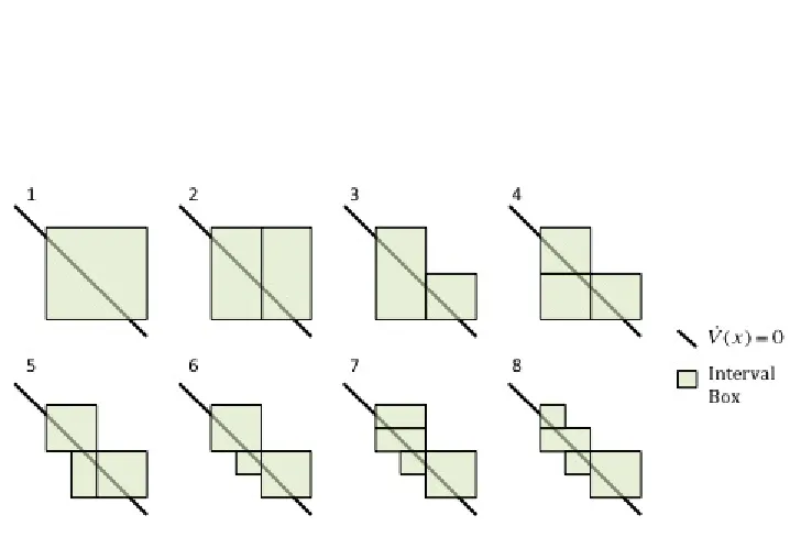
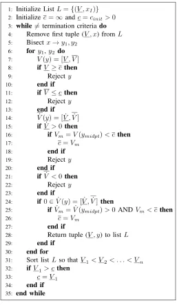
To solve for c∗, from (3.1), the following algorithm, as seen in [45] is implemented:

Initialization:Add the box [0,1]x[0,1]x...x[0,1] and the interval extension of V(x) to a list. Initialize the bounds on c = [c, c] so that c = ∞ and c = cinit where cinit is some

value greater than zero.

Step One:Remove the first box from the list and bisect it. For the two resulting boxes, calculate the interval extensions of the V(x) and ˙V(x) functions.

Step Two:If the interval extension of ˙V(x) = [ ˙V ,V˙] contains ˙V(x) = 0, i.e. ˙V <0 and ˙

V >0, then the interval box and the associated V is returned to the list. Otherwise the interval will be discarded.

Step Three:Solve for a new upper bound of c. For intervals that are being re-added to the list, if ˙Vm >0 ANDVm < c, where ˙Vm and Vm are the values of ˙V and V evaluated

at the midpoint of the interval, thenc=Vm. If the interval is being rejected and if ˙V >0

AND Vm < c then setc=Vm. Otherwisec does not change.

Step Four:Once all intervals have either been added to the list are discarded, the list is sorted so that the interval with the smallest V is first and the interval with the largest V is last. IfV of the first interval in the list is less than c, then cis reset to that value.

Step Five: Repeat steps one through 4 until a user-defined termination criteria, e.g. c−c < , is fulfilled.

These steps are further outlined in Figure 3.2.

3.2 Two State Model

(39)

and Wee1 protein interaction, which is a key interaction in cell cycle regulation. Figure

3.3 shows the simplified mutually inhibitive Cdc2-cyclin B and Wee1 model. This model

was chosen because it exhibits bistability characteristics under certain parameters. This

is useful for our purpose since there will be a minimum of two biologically relevant stable

equilibrium points. This is useful to know, because it allows us to examine the ROA

estimation algorithm for an equilibrium point that is not globally stable.

The Cdc2-cyclin B complex and Wee1 protein interaction from Figure 3.3 can be

described in continuous Boolean form as shown in (3.2) [3]. Here, x is Cdc2-cyclin B complex and y is Wee1 protein. Here, τx = 1, τy = 10, kx = 0.1, and ky = 0.3. The

calculated Lyapunov function associated with the equilibrium point at [1 0]T _{is shown}

in (3.3). The P matrix associated with (3.3) was found using the Matlab LMI Control Toolbox [17].

˙ x= 1

τx

_k4

y

y4₊_k4 y

−x

˙ y = 1

τy

k_x4 x4₊_k4

x

−y

(3.2)

V(x) =xTPx= 0.9315x2+ 1.7914y2 −0.0000825xy. (3.3) The corresponding ˙V(x) is:

˙

V(x) = −1.863x2−0.358y2+ 0.00009xy−0.000008x+ 0.3583y (3.4) +B1 −1.863x+ 0.00008y

+B2 0.000008x−0.358y

(40)

where,

B1 =

y4

y4₊_k4 y

B2 =

x4

x4₊_k4 x

.

This Lyapunov function and its time derivative were used to implement the interval

ROA estimation procedure shown in Figure 3.2 using the Boost C++ Interval Library

[4]. Chapter 4 Section 1 describes the results obtained using this method.

Figure 3.3: Schematic depiction of the simplified Cdc2-cyclin B/Wee1 mutually in-hibitory system [3]

3.3 Three State Model

The 3 state Hillcube model used in this work comes from a subnetwork of the Rb-E2F

signaling pathway shown in Figure 3.4b. The Rb-E2F pathway regulates the initiation

of DNA replication and plays a critical role in cell proliferation by acting as a bistable

switch that converts graded growth signals into an all-or-none activation of E2F [50].

(41)

(a)

(b) (c)

(42)

that this pathway is deregulated in almost all cancer cells [31][46]. Yao et. al. identified a

minimal circuit that generates robust, resettable bistability. Experimental disruption of

this circuit abolishes maintenance of the activated E2F state, supporting its importance

for the bistability of the Rb-E2F system [50]. In this work, the ROA estimation technique

outlined in Figure 3.2 is applied to this minimal circuit of the Rb-E2F pathway, shown

in Figure 3.4c. Hillcube approximations are used to describe this network and are shown

in (3.6). d[MD] dt = 1 τm

[S]n1

[S]n1 ₊_kn1

s −[MD] d[RP] dt = 1 τr

kn2

m1

[MD]n2 ₊_kn2

m1

· k

n3

e

[EE]n3 ₊_kn3

e −[RP] (3.6) d[EE] dt = 1 τe

[MD]n4

[MD]n4 ₊_kn4

m2

· k

n5

r

[RP]n5 ₊_kn5

r

−[EE]

.

Here, τm = τr = τe = 1, ks = 0.8, km1 = 0.7, km2 = 0.02, ke = 0.3, kr = 0.03,

the input, S, is fixed to 1, and ni = n = 4 ∀ 1 ≤ i ≤ 5. The system above has three

equilibrium points, two stable nodes, and a saddle point. Without loss of generality we

examine the ROA of the stable node

xe ye ze

T

=

0.7094 0.4866 0.000014

T

. The

nature of the Lyapunov function requires that the stable equilibrium occurs at the origin,

so it is necessary to translate the system so that the stable node is at the origin. For the

(43)

and [EE] will be expressed as z. The translated system becomes:

˙

x= 1 1 +kn

s

−x ˙

y= k

n m1

xn₊_kn m1

· k

n e

zn₊_kn e

−y (3.7)

˙

z = x

n

xn₊_kn m2

· k

n r

yn₊_kn r

−z.

For the system shown in (3.7), the following Lyapunov function satisfying (2.13) was

calculated using the LMI solver in Matlab’s Control Toolbox [17]:

V(x) = 57.85x2+ 32.25y2+ 36.81z2+ 37.32xy

+ 0.0014xz+ 0.0032yz (3.8)

The time derivative of the Lyapunov function (3.8) is calculated as:

˙

V(x) = −115.69x2−64.50y2−73.63z2−74.66xy

−0.0028xz−0.0064yz−18.16x−31.385y (3.9)

−0.0026z+B1(37.33x+ 64.50y+ 0.0032z)

(44)

where,

B1 =

kn m1

xn₊_kn m1

· k

n e

zn₊_kn e

B2 =

xn

xn₊_kn m2

· k

n r

yn₊_kn r

.

This Lyapunov function and its time derivative were used to implement the interval ROA

estimation procedure shown in Figure 3.2 using the Boost C++ Interval Library [4]. The

results of this algorithm are described in Chapter 4 Section 2.

3.4 Expanding the Calculated Estimate

The available LMI solvers calculate a P matrix that meets the requirements of the LMI constraints, (2.13). The resulting matrix is always feasible, but is not always the“best”

Lyapunov function for providing the largest estimate of the ROA. There exists a

po-tentially infinite number of Lyapunov functions that can satisfy the necessary LMI

con-straints. Each of these quadratic Lyapunov functions represent an ellipse on the phase

plane. The underlying flow of the system, however, makes some Lyapunov functions more

appropriate than others in terms of identifying the largest possible estimate of the ROA.

In our approach we use mechanisms for controlling the elongation and rotation of the

corresponding ellipse to identify a larger estimate of the ROA.

This algorithm will first look at rotating the given P matrix to find the orientation that gives the largest estimate of the ROA for that ellipsoid. Then, by adjusting the

eigenvalues of the rotated P matrix, the algorithm will change the shape of the ellipsoid to find the one that works best with the system dynamics. The LMI constraints in (2.13)

(45)

Figure 3.5

systems whose trajectories approach the equilibrium point in a circular fashion, a more

circular Lyapunov region would provide a larger estimate than an elongated ellipse. For

systems like the two state example in section 3.2 represented by (3.2), a longer ellipse

would have a larger estimate of the ROA than a circular region. For each change in the

ellipsoid, the interval analysis ROA estimation algorithm, Figure 3.2, is re-run to find

the largest level set.

To determine how different orientations and shapes of an ellipse can change the size

of the ROA estimate, we looked at the bistable 2 dimensional system presented in

sec-tion 3.2. Using the P matrix returned by the LMI solver, we evaluated several different orientations, includingθ= 15◦, 30◦, and 45◦, whereθ increases in the clockwise direction from the x-axis as shown in Figure 3.5.

The P matrix is rotated in the clockwise direction using the following formula:

Pθ =RθP RTθ where, Rθ =



 

cos(θ) sin(θ)

−sin(θ) cos(θ)





(46)

(a) (b)

(47)

Once the original ellipse is rotated θ◦, Vθ is used to calculate a new ˙Vθ(x). These

functions are then used to calculate the largest level set c∗_θ for that orientation. Figure 3.6a shows three different orientations of the same Lyapunov function. The purple and

green ellipses are rotations of the initial ellipse (orange). Figure 3.6a shows that both of

these rotations allow for larger level sets of the ellipse to be used as the ROA estimate.

The ratio of the eigenvalues of theVθ that gives the largest ROA estimate are adjusted

to vary the shape of the ellipse. The eigenvalues determine the size of the major and minor

axes of the ellipse. Since we are looking at different level sets of the ellipses, the individual

values of the eigenvalues are not important. Instead, the ratio between eigenvalues is what

we are interested in, as this determines whether the ellipse is circular or long and skinny.

Figure 3.6b shows an initial ellipse (green) is the same ellipse which gave the largest

ROA estimate from Figure 3.6a. The eigenvalues of this ellipse are adjusted to produce a

skinnier ellipse (red) and a more circular ellipse (blue). Figure 3.6b shows that the largest

(48)

Chapter 4 Results

In this chapter we present and discuss the results of the interval analysis ROA estimation

algorithm on the two and three state biological models presented in Chapter 3. We

then look at our preliminary findings from the discussed method of determining better

Lyapunov functions in Chapter 3 Section 3. The plots shown in Figures 4.1 -4.4 were

produced using Mathematica [49].

4.1 Two State Model

Figure 4.1a shows the phase portrait of the two state system described in (3.2) with

sam-ple trajectories. The solid gray line represents the boundary ˙V(x) = 0 and the solid black curve (without arrows) defines the boundary, c = [0.081,0.082], of the ROA estimation within the shifted Boolean space. The gray point that falls on the curve ˙V(x) = 0 is a saddle point, and the two black points are stable nodes. The solid black trajectories

converge to the stable point [1 0]T _{inside the ROA estimate. The dashed trajectories}

(49)

are several initial conditions that reside in the true ROA but are not included in the

calculated estimate. This is a characteristic of Lyapunov based ROA estimates. This

conservativeness of the estimate is due, in part, to the requirement that once a trajectory

enters a Lyapunov function, it must remain inside the Lyapunov function. It is not

un-common, however, for trajectories to leave and then re-enter the Lyapunov region, but it

is impossible to analytically determine which trajectories re-enter the Lyapunov region,

and which trajectories are not elements of the actual ROA. Figure 4.1b illustrates this.

Two initial conditions are chosen close together and both of the trajectories leave the

level setV(x)≤c= 1.1. One of the trajectories re-enters the region and converges to the desired stable equilibrium point. The other trajectory, however, converges to the second

equilibrium point. For this reason, it is necessary to constrain the ROA estimate to the

level set that is tangent to line ˙V(x) = 0.

4.2 Three State Model

The ROA estimation approach shown in Figure 3.2 returned the following bounds forc∗,

c= [c, c] = [6.2828,6.2832]

Figure 4.2 shows sample trajectories of system (3.7). The solid black curves are

tra-jectories that converge to the analyzed stable point, and the dashed black curves are

trajectories that converge to the second stable point. As seen in this figure, there are

ini-tial conditions outside of our estimated ROA that still converge to the equilibrium point.

Clearly, the estimated ROA is only a subset of the actual ROA, in the same manner as the

(50)

(a)

(b)

(51)

(52)

a trajectory that starts in the ˙V(x)>0 region but eventually converges to the selected equilibrium point. Since the stability characteristics of the ROA estimate in the 3 state

example are congruent to the characteristics discussed in the 2 state example, it can be

extrapolated that these characteristics will remain regardless the size of the system, and

therefore, this method is applicable to not only to 2 and 3 dimensional systems, but also

higher dimensional systems whose phase plane cannot be visualized.

Knowing the ROA, or at least an estimate of the ROA is an important stability

characteristic in nonlinear dynamics. The ROA characterizes all of the initial conditions

that converge to a specified equilibrium point. An estimate of the ROA provides a group

of initial conditions whose trajectories are guaranteed to converge to the desired stable

point. This is important information when a particular stable characteristic is desired.

For the Rb-E2F biochemical pathway, it may be of interest to ’manually’ turn the E2F

’On’ ([EE]≈1) or ’Off’ ([EE]≈0). This could be achieved by increasing or decreasing the concentration levels of the components until they reside in the known estimated ROA.

This would guarantee that the desired steady state of the system is achieved.

The applicability of this approach to higher dimensional systems is an important

quality when considering analysis techniques for biological systems, since the majority

of biological systems are large and have many states. The examples in this paper were

simplifications of larger biological models, and were reduced to 2 and 3 states respectively

for visualization purposes. The Lyapunov function shown in (2.11), however, can be

defined for n >3 dimensions. This would allow us to obtain the corresponding level set, c, for the ROA estimate in larger dimensions. Parallelization methods would decrease the computation time of the interval approach to such larger dimensions [26].

The better the estimate of the ROA, the better the understanding of which initial

(53)

are needed to increase the estimate of ROAs associated with non-polynomial systems.

Since the shape of the surface ˙V(x) = 0 is dependent on the specific Lyapunov function, one potential method for increasing an ROA estimate is to take the union of several

Lyapunov ROA estimates to increase the total ROA estimate of an equilibrium point.

Qualitatively similar techniques have been proposed for polynomial systems but have not

been applied to non polynomial nonlinear systems [11][40].

4.3 Expanding Calculated Estimate: Preliminary

Re-sults

Below are the preliminary results found when looking at rotating and changing the size

and shape of the P matrix given by the LMI solver.

4.3.1 Rotate

V

We took the calculated Lyapunov function from section 4.1 and rotated it around the

equilibrium point calculating the largest level sets for the different orientations. Figure

4.3 shows the initial estimate calculated in section 4.1 and the largest level sets of that

Lyapunov function rotated 15◦, 30◦, and 45◦ from the x-axis. As seen in this figure, when the Lyapunov function is rotated 15◦ from its original position, it covers a larger area of the system space than the other orientations. This information is tabulated in Table 4.1,

(54)

(55)

Table 4.1: The area of the ROA estimate when the given P matrix is rotated about the equilibrium point

θ c∗ Area P

0◦ 0.081 0.0413

0.9315 −4.1277×10−5

−4.1277×10−5 _1.7914

15◦ 0.088 0.0506

0.9891 0.2149 0.2149 1.7338

30◦ 0.075 0.0492

1.1464 0.3723 0.3723 1.5763

45◦ 0.0565 0.0414

1.3614 0.4299 0.4299 1.3615

4.3.2 Alter Shape of

V

Next we looked at scaling the eigenvalues of V15◦ to see how changing the shape of the ellipse can change to size of the estimate. We scaled the eigenvalues to create an ellipse

that was narrower than the original and one that was more circular. Figure 4.4 shows

the three ellipses, where the largest estimate from section 4.3.1, V15◦, is shown in red. As can be seen, the narrower ellipse, in purple, has a significant increase of area than the

others. Table 4.2 lists the specifications of each of the three regions. The largest estimate

has an area of 0.1030, which is an increase of 147% from the original estimate found in

section 4.1. Figure 4.5 shows the boundary of the actual ROA along with the original

estimate (blue) and the larger estimate (purple) found through rotating and scaling the

dimensions of the ellipse. In this figure, the actual ROA is the area below the stable

(56)

Figure 4.4: Three different ROA estimates oriented atθ = 15◦. The dashed curves mark ˙

(57)

(58)

Table 4.2: The ROA Estimate with the largest area from Table 4.1 (θ = 15◦) and two additional estimates that result from changing the eigenvalues of that Lyapunov function.

Eigenvalues of Ellipse (λ) c∗ Area P

λ1 = 0.9315, λ2 = 1.7914 0.088 0.0506

0.9891 0.2149 0.2149 1.7914

λ1 =2.045, λ2 =8.2240 0.63 0.1030

2.4588 1.5445 1.5445 7.8102

λ1 = 3.2, λ2 = 5.1 0.23 0.0431

3.3272 0.4749 0.4749 4.9728

These preliminary results show that depending on the Lyapunov function that the

LMI solver returns, the ROA estimate can vary in size. The larger the estimate that can

be found, the better and therefore, we conclude it is worthwhile to proceed with this

research and develop an algorithm that will determine better Lyapunov functions for a

(59)

Chapter 5 Conclusion

5.1 Conclusion

This thesis addressed the issue of whether the ROA estimation algorithm outlined in

Figure 3.2 [45] is suitable for biochemical systems modeled using continuous Boolean

Hillcube approximations. We applied the method to two models, a two state Cdc2-cyclin

B complex and Wee1 protein interaction and a three dimensional model of the Rb-E2F

pathway. We showed that the interval analysis ROA estimation technique provided an

accurate estimate of the ROA for both systems. In both cases, the estimated ROA is on

par with accuracy of other ROA estimates in the literature that use Lyapunov stability.

We conclude that this method is a viable technique for estimating the ROA of biological

systems modeled with continuous Boolean Hillcube approximations.

We also began looking at how different Lyapunov functions can affect the size of the

estimated ROA. We showed that there can be a significant improvement in the size of

the ROA estimate by rotating and changing the shape of the ellipse given by the LMI

(60)

changes.

5.2 Future Work

5.2.1 Develop Algorithm to Find Best Quadratic Lyapunov

Func-tion

Based on the preliminary results of trying to find larger quadratic functions, the next

step is to develop an algorithm that will find the best shape and orientation of the

quadratic ROA estimate based on the system. Since this algorithm has the potential

to be computationally intensive, we will look at using a genetic algorithm to determine

which angles and eigenvalues will be used to find the largest quadratic Lyapunov function.

The goal of the genetic algorithm will be to narrow in on the best values without having

to run through every single value.

5.2.2 Increase ROA Estimate

The long term goal of my research is to be able to determine how climate change affects

the stability of physical characteristics in plants. In order for this to be accomplished,

however, there must be significant improvement on the current methods of estimating

regions of attraction to get an accurate representation of how the regions of attraction

of the phenotypes are affected by changes in the environment. The current elliptical

estimates found using quadratic Lyapunov functions are generally too conservative for

the information to be very useful. One possible method that has been briefly explored by

researchers include looking at the union of several quadratic Lyapunov functions [11][40].

(61)

be too conservative. Another idea is to use concepts from computational geometry such

as free-form deformation and morphing to expand a quadratic region of attraction into

a larger region depending on the system flow. This would mean that the ROA estimate

would no longer be constrained to a quadratic function allowing for the potential of a

much larger estimate of the ROA. Figure 5.1 shows an example of how this expansion

might occur using a geometrical mesh and expanding individual points on the boundary

of the region until the trajectories begin leaving the region.

(62)

REFERENCES

[1] I. Ahuja, R.C.H. De Vos, A.M. Bones, and R.D. Hall. Plant molecular stress re-sponses face climate change. Trends in plant science, 15(12):664–674, 2010.

[2] R. Albert and H.G. Othmer. The topology of the regulatory interactions predicts the expression pattern of the segment polarity genes in drosophila melanogaster.

Journal of Theoretical Biology, 223(1):1–18, 2003.

[3] D. Angeli, J.E. Ferrell, and E.D. Sontag. Detection of multistability, bifurcations, and hysteresis in a large class of biological positive-feedback systems. Proceedings of the National Academy of Sciences of the United States of America, 101(7):1822, 2004.

[4] Herv´e Br¨onnimann, Guillaume Melquiond, and Sylvain Pion. The design of the boost interval arithmetic library, 2006.

[5] E.C. Butcher, E.L. Berg, and E.J. Kunkel. Systems biology in drug discovery.Nature biotechnology, 22(10):1253–1259, 2004.

[6] G. Chesi. Computing output feedback controllers to enlarge the domain of attraction in polynomial systems. Automatic Control, IEEE Transactions on, 49(10):1846– 1853, 2004.

[7] G. Chesi. Estimating the domain of attraction for uncertain polynomial systems.

Automatica, 40(11):1981–1986, 2004.

[8] G. Chesi. Estimating the domain of attraction for non-polynomial systems via lmi optimizations. Automatica, 45(6):1536–1541, 2009.

[9] G. Chesi. Robustness analysis of genetic regulatory networks affected by model uncertainty. Automatica, 47(6):1131–1138, 2011.

[10] G. Chesi, L. Chen, and K. Aihara. On the robust stability of time-varying uncertain genetic regulatory networks. International Journal of Robust and Nonlinear Control, 2011.

[11] Graziano Chesi. Estimating the domain of attraction via union of continuous families of lyapunov estimates. Systems; Control Letters, 56(4):326–333, 2007.

(63)

[13] M.I. Davidich and S. Bornholdt. Boolean network model predicts cell cycle sequence of fission yeast. PLoS One, 3(2):e1672, 2008.

[14] P. ´Erdi and J. T´oth. Mathematical models of chemical reactions: theory and ap-plications of deterministic and stochastic models. Manchester University Press ND, 1989.

[15] A. Faur´e, A. Naldi, C. Chaouiya, and D. Thieffry. Dynamical analysis of a generic boolean model for the control of the mammalian cell cycle. Bioinformat-ics, 22(14):e124–e131, 2006.

[16] E.D. Ferreira and B.H. Krogh. Using neural networks to estimate regions of stability. In American Control Conference, 1997. Proceedings of the 1997, volume 3, pages 1989–1993. IEEE, 1997.

[17] P. Gahinet, A. Nemirovskii, A.J. Laub, and M. Chilali. The lmi control toolbox. In

Decision and Control, 1994., Proceedings of the 33rd IEEE Conference on, volume 3, pages 2038–2041, dec 1994.

[18] R. Genesio, M. Tartaglia, and A. Vicino. On the estimation of asymptotic stability regions: State of the art and new proposals. Automatic Control, IEEE Transactions on, 30(8):747–755, 1985.

[19] L. Jaulin.Applied interval analysis: with examples in parameter and state estimation, robust control and robotics, volume 1. Springer Verlag, 2001.

[20] H. Kitano. Systems biology: a brief overview. Science, 295(5560):1662–1664, 2002.

[21] E. Klipp. Systems biology in practice: concepts, implementation and application. Vch Verlagsgesellschaft Mbh, 2005.

[22] A.K. Konopka. Systems biology: principles, methods, and concepts. Crc, 2007.

[23] M. Lhommeau, L. Jaulin, and L. Hardouin. Capture basin approximation using interval analysis. International Journal of Adaptive Control and Signal Processing, 25(3):264–272, 2011.

[24] F. Li, T. Long, Y. Lu, Q. Ouyang, and C. Tang. The yeast cell-cycle network is robustly designed. Proceedings of the National Academy of Sciences of the United States of America, 101(14):4781, 2004.

(64)

[26] S. Mayer, B. Tibken, and S. Warthenpfuhl. Parallel computation of domains of attraction for nonlinear dynamic systems. In Parallel Computing in Electrical En-gineering (PARELEC), 2011 6th International Symposium on, pages 87–92. IEEE, 2011.

[27] A. Merola, C. Cosentino, and F. Amato. An insight into tumor dormancy equilib-rium via the analysis of its domain of attraction. Biomedical Signal Processing and Control, 3(3):212–219, 2008.

[28] R.E. Moore. Interval analysis, volume 60. Prentice-Hall Englewood Cliffs, NJ, 1966.

[29] R.E. Moore, R.B. Kearfott, and M.J. Cloud. Introduction to interval analysis. So-ciety for Industrial Mathematics, 2009.

[30] A. Mukhopadhyay, A.M. Redding, B.J. Rutherford, and J.D. Keasling. Importance of systems biology in engineering microbes for biofuel production. Current opinion in biotechnology, 19(3):228–234, 2008.

[31] J.R. Nevins. The rb/e2f pathway and cancer.Human Molecular Genetics, 10(7):699– 703, 2001.

[32] J.C. Polking. Rice university, pplane, 2009.

[33] C.V. Rao and A.P. Arkin. Stochastic chemical kinetics and the quasi-steady-state assumption: Application to the gillespie algorithm. The Journal of chemical physics, 118:4999, 2003.

[34] S. Ratschan and Z. She. Providing a basin of attraction to a target region by computation of lyapunov-like functions. InComputational Cybernetics, 2006. ICCC 2006. IEEE International Conference on, pages 1–5. IEEE, 2006.

[35] P. Sannigrahi, A.J. Ragauskas, and G.A. Tuskan. Poplar as a feedstock for biofuels: A review of compositional characteristics. Biofuels, Bioproducts and Biorefining, 4(2):209–226, 2010.

[36] M.A. Stadtherr, G. Xu, G.I. Burgos-Solorzano, and W.D. Haynes. Reliable com-putation of phase stability and equilibrium using interval methods. International Journal of Reliability and Safety, 1(4):465–488, 2007.

[37] Steven H Strogatz. Nonlinear Dynamics And Chaos: With Applications To Physics, Biology, Chemistry And Engineering. Westview Press, 1994.

(65)

[39] B. Tibken. Estimation of the domain of attraction for polynomial systems via lmis. In

Decision and Control, 2000. Proceedings of the 39th IEEE Conference on, volume 4, pages 3860–3864. IEEE, 2000.

[40] B. Tibken and Y. Fan. Computing the domain of attraction for polynomial systems via bmi optimization method. In American Control Conference, 2006, pages 6–pp. IEEE, 2006.

[41] U. Topcu, A. Packard, and P. Seiler. Local stability analysis using simulations and sum-of-squares programming. Automatica, 44(10):2669–2675, 2008.

[42] W. Tucker. The lorenz attractor exists.Comptes Rendus de l’Acad´emie des Sciences-Series I-Mathematics, 328(12):1197–1202, 1999.

[43] J.J. Tyson, K. Chen, B. Novak, et al. Network dynamics and cell physiology. Nature Reviews Molecular Cell Biology, 2(12):908–916, 2001.

[44] AR Tzafriri. Michaelis-menten kinetics at high enzyme concentrations. Bulletin of mathematical biology, 65(6):1111–1129, 2003.

[45] S. Warthenpfuhl, B. Tibken, and S. Mayer. An interval arithmetic approach for the estimation of the domain of attraction. In Computer-Aided Control System Design (CACSD), 2010 IEEE International Symposium on, pages 1999–2004, sept. 2010.

[46] R.A. Weinberg. The biology of cancer, volume 255. Garland Science New York, 2007.

[47] Dominik Wittmann, Jan Krumsiek, Julio Saez-Rodriguez, Douglas Lauffenburger, Steffen Klamt, and Fabian Theis. Transforming boolean models to continuous mod-els: methodology and application to t-cell receptor signaling. BMC Systems Biology, 3(1):98, 2009.

[48] Dominik M. Wittmann, Florian Bl¨ochl, Dietrich Tr¨umbach, Wolfgang Wurst, Nilima Prakash, and Fabian J. Theis. Spatial analysis of expression patterns predicts genetic interactions at the mid-hindbrain boundary. PLoS Comput Biol, 5(11):e1000569, 11 2009.

[49] Stephen Wolfram. Mathematica for students.

Region of Attraction Estimation of Biological Continuous Boolean Models.

ABSTRACT

DEDICATION

BIOGRAPHY

ACKNOWLEDGEMENTS

TABLE OF CONTENTS

LIST OF TABLES

LIST OF FIGURES

Chapter 1

Introduction

1.1

Overview

1.2

Motivation

1.3

Contributions of this Work

1.3.1

Intellectual Merit

1.3.2

Broader Impacts

1.4

Organization

Chapter 2

Background

2.1

Modeling Biological Pathways

2.1.1

Mass Action Kinetics

2.1.2

Michaelis-Menten Kinetics

2.1.3

Boolean Modeling

2.2

Interval Arithmetic

2.3

Estimating Regions of Attraction

2.3.1

Lyapunov Functions

2.3.2

ROA Estimation for Nonlinear Polynomial Functions

2.3.3

ROA Estimation for Nonlinear Non-Polynomial Functions

Chapter 3

Methodology

3.1

Interval ROA Estimation Method

3.2

Two State Model

3.3

Three State Model

3.4

Expanding the Calculated Estimate

Chapter 4

Results

4.1

Two State Model

4.2

Three State Model

4.3

Expanding Calculated Estimate: Preliminary

Re-sults

4.3.1

Rotate

V

4.3.2

Alter Shape of

V

Chapter 5

Conclusion

5.1

Conclusion

5.2

Future Work

5.2.1

Develop Algorithm to Find Best Quadratic Lyapunov

Func-tion

5.2.2

Increase ROA Estimate

REFERENCES