Abstract
JAFARI, REZA. Safety Effects of the Access Points near Signalized Intersections. (Under the direction of Dr. Joseph E. Hummer.)
In the US in 2009, 5.5 million collisions occurred in which over 2.2 million people were injured and over 33,000 people died due to highway collisions. Over half of these total crashes were intersection and access point – related. Most collision reporting systems do not provide the necessary level of information to identify access – related collisions but collision data, where available, indicate a high incidence of access – related collisions.
The objectives of this research were to develop a valid statistical model to estimate the number of access point – related collisions occurring at access points near signalized intersections and providing checklist for site planners and decision-makers to distinguish higher collision sites from lower collision sites and avoid constructing higher collision sites.
Geometric, traffic, and access – related collision data over 5 years, from January 2005 to December 2009 were collected for 108 sites. Out of the 15 independent variables tested, only AADT, driveway width, and Synchro through movement 95% queue at the intersection near the access point were statistically significant in developing the collision prediction statistical model. This model could be used by state DOTs and municipal traffic engineers to address access management requirements and to predict problems likely to result from site traffic impacts. To provide checklist for site planners to distinguish the higher collision sites from lower collision sites, the data that were previously collected and some new information such as demographic and socio economic data were used. The higher collision sites were investigated one by one.
Safety Effects of the Access Points near Signalized Intersections
by Reza Jafari
A dissertation submitted to the Graduate Faculty of North Carolina State University
in partial fulfillment of the requirements for the Degree of
Doctor of Philosophy
Civil Engineering
Raleigh, North Carolina
2011
APPROVED BY:
___________________ __________________ _________________ Dr. Nagui M. Rouphail Dr. Billy M. Williams Dr. John F. Monahan
ii
Dedication
This work is dedicated to my mother, who loves me unconditionally, to my father, who has taught me how to work hard and is proud of me, and to the color of my life, Zohreh, without whose caring support it would not have been possible. This work is also
iii
Biography
Reza Jafari is a civil engineering alumna from Northeastern University in Boston, Massachusetts with a Master of Science degree. He also got a Bachelor of Science degree from Sharif
University of Technology and a Master of Science degree from K.N.T. University, both in Mechanical Engineering from Tehran, Iran.
Reza has over seven years of experience in transportation and traffic engineering. He worked for WSP-SELLS and the Congestion Management Unit of the North Carolina Department of
Transportation (NCDOT) and on a few projects at North Carolina State University and Northeastern University. He worked on different projects including safety analysis, signal design, capacity analysis, traffic impact analysis, parking studies, pedestrian access improvements, and roadway improvements for public and private clients.
Reza held teaching assistant and research assistant positions while pursuing his MSc and Ph.D. in Civil Engineering at Northeastern University and North Carolina State University. In North Carolina State University and under the direction of Professor Joseph Hummer, he participated in a research project sponsored by the NCDOT to evaluate a railroad crossing wayside horn and in research to analyze the safety effects of the access points near signalized intersections.
iv
Acknowledgements
Any findings, conclusions, and recommendations expressed in this dissertation research are those of the author and do not necessarily reflect the views of the people and organizations with whom I would like to acknowledge for their gracious support.
I cannot really find the right words to express my sincere gratitude and appreciation to Dr. Joseph Hummer who was not only my advisor throughout the process of this dissertation, but also a good friend. His intelligence, guidance, inspirational encouragement, advice, continuous support, and patience have been of the utmost importance to the completion of my research work.
I would like to thank my friend and former classmate, Dr. Jongdae Baek whose research was very helpful in developing my statistical analysis. His friendship and technical suggestions on this research was invaluable.
I would like to express my gratitude to my committee members, Dr. Nagui Rouphail, Dr. John Monahan, and Dr. Billy Williams and also to Dr. John Stone whose precious suggestions and continuous support helped me to improve the quality of this research document and analyses.
My special thanks go to Dr. Ezra Hauer who always had responded to my questions in a timely manner with comprehensive detailed information. His statistical analyses were used as the basis of this research. Not only me, but the entire society of roadway safety, worldwide appreciate his effort in producing valuable research to be used now and in the future by safety professionals to reduce road collisions and ultimately save more lives.
This research was initially generated by the help of my former supervisor at NCDOT, James Dunlop. He was very supportive and assisted me with obtaining some of the necessary data required for this study. I also extend my appreciation to Kevin Lacey and Jeff Jaeger of the NCDOT for their permission in using the North Carolina traffic collision database.
v
I would like to express my special appreciation to Phil Demosthenes, Bernie Kalus of WSP-Sells, Lori Cove of the Town of Cary, John Albeck of the Trafficware, Kent Taylor and Byron Sanders of the NCDOT, and Kyle Ward of the North Carolina Capital Area MPO who provided me with turning counts and other valuable traffic data used in this study. I also would like to thank Bowman Kelly of the City of Raleigh who provided me with traffic volume data and supported me since the first day I met him at NC State University.
I would like to thank the North Carolina Section of the ITE for supporting me with their scholarship that encouraged me to stay, work, and complete my PhD degree in Transportation Engineering.
I would like to thank my former advisor, Dr. Honarvar who taught me to “see the cup as half full”. I also deeply appreciated all the assistance from my teacher, Dr. Sadati in helping me finding my path, and discovering better ways to be more helpful to myself and my society. Dr. Sadati was more than a teacher to me. He is, and was, my mentor, older brother, and a blameless friend.
My special appreciation is extended to my friends and coworkers, Dr. Majed Al-Ghandour, Dr.-to-be Katy Salamati, Anne Holzem, Dr. Elizabeth Harris, Mike Reese, Dr.-Dr.-to-be Leta
Huntsinger, Dr. Bastian Schroeder, Dr. Daniel Findley, Dr. Alix Demers, Erin Harrington, Caroline Kone, Mike Surasky, Gavin Teng, Avani Patel, Dr. Jae Pil Moon, Dr. Hyejun Hu for their continuous support.
I would like to express my heartfelt thanks to my parents and my brothers for their love and great support for my education. Without their endless encouragement, this work could not have been possible.
vi
Table of Contents
List of Figures ... x
List of Tables ...xiii
1. INTRODUCTION ... 1
1.1 Background ... 1
1.2 Objective ... 2
1.3 Scope ... 3
1.4 Organization ... 5
2. LITERATURE REVIEW ... 6
2.1 Driveways ... 6
2.2 Access management ... 7
2.3 Corner clearance ... 11
2.4 Collision models ... 12
3. DATA PREPARATION ... 17
3.1 Site selection ... 17
3.2 Data collection ... 24
3.2.1 Geometric data ... 24
3.2.2 Traffic data ... 25
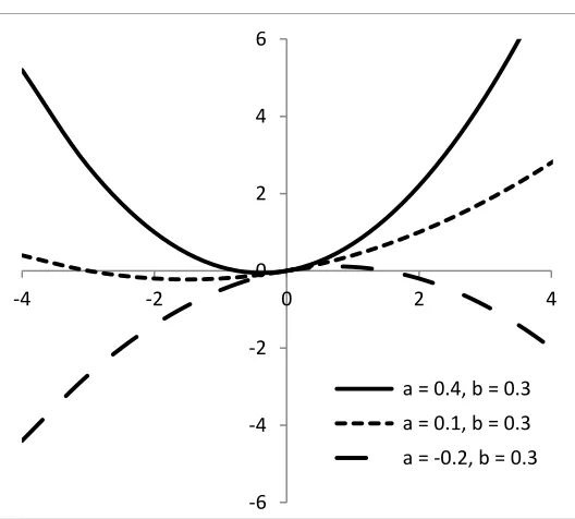
3.2.3 Collision data ... 32
3.3 Data analysis ... 35
3.3.1 Corner clearance ... 35
3.3.2 Lane configuration at the intersection ... 36
3.3.3 Lane configuration at the driveway... 36
3.3.4 Major road median type ... 37
3.3.5 Speed limit on the major road ... 37
3.3.6 Grade on the major road... 38
3.3.7 Driveway angle ... 38
3.3.8 Driveway one-way or two-way operations ... 40
vii
3.3.10 Driveway median status ... 40
3.3.11 Driveway width ... 41
3.3.12 Transition ... 41
3.3.13 Driveway radius ... 42
3.3.14 Second driveway ... 43
3.4 Summary of data ... 43
4. ANALYSIS METHODOLOGY ... 44
4.1 Modeling method ... 45
4.1.1 Data traits ... 45
4.2 Modeling Process ... 47
4.2.1 Candidate functional forms ... 49
4.2.2 Integrate – differentiate method ... 51
4.2.3 Estimation of the model coefficients... 54
4.2.4 Model selection ... 59
4.3 Goodness of fit ... 62
5. MODELING PROCESS ... 65
5.1 Initial model ... 65
5.2 Second model ... 67
5.2.1 Driveway volume ... 68
5.2.2 Corner clearance ... 71
5.2.3 Synchro queue length ... 72
5.2.4 Driveway width ... 76
5.2.5 Lane configuration at the intersection ... 78
5.2.6 Lane configuration at the driveway... 79
5.2.7 Grade on the major road... 79
5.2.8 Speed limit ... 79
5.2.9 Major road median ... 80
5.2.10 Driveway median ... 80
5.2.11 Driveway angle ... 81
viii
5.2.13 Transition ... 82
5.2.14 Second driveway ... 82
5.2.15 Result ... 83
5.3 Third model ... 85
5.3.1 Lane configuration at the intersection ... 86
5.3.2 Grade on the major road... 86
5.3.3 Driveway volume ... 87
5.3.4 Through movement Synchro queue ... 89
5.3.5 Result ... 91
5.4 Fourth model ... 93
5.4.1 Major road median ... 93
5.4.2 Lane configuration at the driveway... 94
5.4.3 Speed limit ... 94
5.4.4 Driveway angle ... 94
5.4.5 Second driveway ... 95
5.4.6 Corner clearance ... 95
5.4.7 Driveway radius ... 96
5.4.8 Driveway transition ... 97
5.5 Modeling result ... 97
5.6 Model validation ... 101
6. HIGHER COLLISION SITE IDENTIFICATION ... 104
6.1 Methodology ... 105
6.2 Case studies ... 106
6.2.1 Site 1 ... 107
6.2.2 Site 2 ... 109
6.2.3 Site 3 ... 111
6.2.4 Site 4 ... 113
6.2.5 Site 5 ... 116
6.2.6 Site 6 ... 118
ix
6.3 Analysis... 121
6.3.1 Quantitative variables ... 122
6.3.2 Binary variables ... 123
6.3.3 Driveway left turn proportion ... 124
6.3.4 Categorical variables ... 125
6.3.5 Hourly distribution of collisions ... 126
6.3.6 Socio economics ... 128
6.4 Conclusion ... 130
7. CONTRIBUTING FACTORS ... 131
7.1 Methodology ... 131
7.2 Prediction model ... 132
7.3 Higher collision site identification ... 133
7.4 Conclusion ... 134
8. CONCLUSIONS AND RECOMMENDATIONS ... 137
8.1 Research summary ... 137
8.2 Findings and conclusions ... 138
8.3 Future research recommendations ... 140
References ... 143
Appendices ... 148
Appendix A – Distribution of the study sites in Wake County ... 149
Appendix B – Google Earth Pro daily traffic counts ... 150
Appendix C – Traffic counts data collection method ... 151
Appendix D – Crash Report Form DMV-349 ... 152
Appendix E – Collision IDs ... 154
Appendix F – Summary of study sites and collected data in Wake County ... 165
Appendix G – SAS® Output for Collision Models ... 169
G.1 – Initial Model ... 169
G.2 – Second Model ... 171
x
List of Figures
Figure 1 – Intersection physical and functional areas (7) ... 7
Figure 2 – Driveway upstream of a signalized intersection ... 7
Figure 3 – Corner clearance and radius of the corner on minor street (17) ... 11
Figure 4 – Data preparation overview ... 17
Figure 5 – Wake County in the State of North Carolina (38) ... 18
Figure 6 – (A) Signalized right turn, (B) Free flow right movement ... 19
Figure 7 – Full movement, left-over, and RIRO designs ... 22
Figure 8 – A snapshot of the AADT map (39) ... 25
Figure 9 – Queue on Oneal Road in Raleigh, NC ... 30
Figure 10 – Synchro estimated queue versus observed queue ... 31
Figure 11 – A snapshot of a police report diagram and narrative ... 34
Figure 12 – Corner clearance of the 108 sample sites ... 35
Figure 13 – Corner clearance measurements ... 36
Figure 14 – Driveway angle ... 39
Figure 15 – Short driveway stem ... 40
Figure 16 – Driveways with smooth and elevated transitions ... 42
Figure 17 – Driveways with large and small radii ... 42
Figure 18 – Modeling methodology overview ... 44
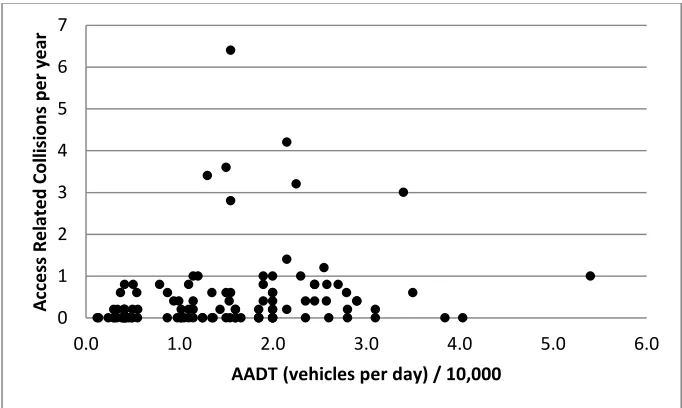
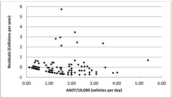
Figure 19 – Correlation between access – related collisions per year and AADT/10,000 ... 47
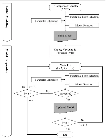
Figure 20 – Modeling methodology overview (46) ... 48
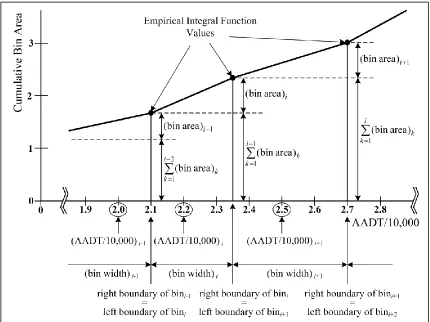
Figure 21 – EIF diagram (46) ... 52
Figure 22 – EIF for the data in Figure 19 ... 52
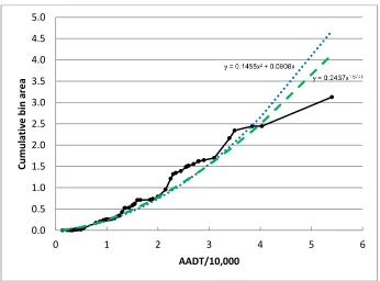
Figure 23 – Example of two candidate functions fitting the cumulative function ... 53
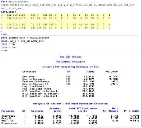
Figure 24 – Codes and output for GENMOD procedures in SAS® ... 56
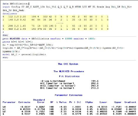
Figure 25 – Codes and output for NLMIXED procedures in SAS® ... 57
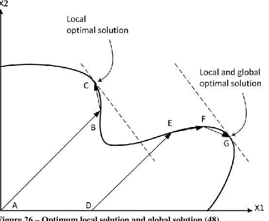
Figure 26 – Optimum local solution and global solution (48) ... 58
Figure 27 – Different graphical behavior of quadratic function of f(x) = ax2+bx ... 59
Figure 28 – Residual plot between annual collected and predicted collisions ... 63
Figure 29 – CURE plot fitted in 2σ* and 2σ* for f(x) = x1.725e- 0.749X ... 64
xi
Figure 31 – Comparison between annual collected and the first model predicted collisions ... 67
Figure 32 – f2(x2) when x2 is the driveway traffic volume ... 69
Figure 33 – EIF of f2(x2) when x2 is driveway traffic volume ... 69
Figure 34 – f2(x2) when x2 is the corner clearance ... 71
Figure 35 – EIF of f2(x2) when x2 is the corner clearance ... 71
Figure 36 – f2(x2) when x2 is the left turn lane Synchro queue ... 73
Figure 37 – f2(x2) when x2 is the through lane Synchro queue ... 73
Figure 38 – f2(x2) when x2 is the right turn lane Synchro queue ... 74
Figure 39 – EIF of f2(x2) when x2 is the Synchro queue for left movement ... 74
Figure 40 – EIF of f2(x2) when x2 is the Synchro queue for thru movement ... 75
Figure 41 – EIF of f2(x2) when x2 is the Synchro queue for right movement ... 75
Figure 42 – f2(x2) when x2 is the driveway width ... 77
Figure 43 – EIF of f2(x2) when x2 is the driveway width ... 77
Figure 44 – CURE plot fitted in 2σ* and 2σ* for second model ... 84
Figure 45 – Comparison between annual collected and the second model predicted collisions ... 85
Figure 46 – f3(x3) when x3 is the driveway traffic volume ... 87
Figure 47 – EIF of f3(x3) when x3 is the driveway traffic volume ... 88
Figure 48 – f3(x3) when x3 is the through movement Synchro queue ... 89
Figure 49 – EIF of f3(x3) when x3 is the trough movement Synchro queue ... 90
Figure 50 – CURE plot fitted in 2σ* and 2σ* for third model ... 92
Figure 51 – Comparison between annual collected and the third model predicted collisions ... 92
Figure 52 – f4(x4) when x4 is the corner clearance ... 95
Figure 53 – EIF of f4(x4) when x4 is the corner clearance ... 96
Figure 54 – Prediction model residuals versus predicted annual access – related collisions ... 98
Figure 55 – Predicted versus observed annual access – related collisions... 99
Figure 56 – Model validation (predicted versus observed annual access – related collisions) ... 103
Figure 57 – Higher collision site identification overview ... 105
Figure 58 – Site 1 aerial image ... 107
Figure 59 – Site 1 collision diagram ... 108
Figure 60 – Site 2 aerial image ... 109
Figure 61 – Site 2 collision diagram ... 110
xii
Figure 63 – Site 3 aerial image ... 112
Figure 64 – Site 3 collision diagram ... 113
Figure 65 – Site 4 aerial image ... 114
Figure 66 – Site 4 collision diagram ... 115
Figure 67 – Site 4 access point exit issues ... 115
Figure 68 – Site 5 aerial image ... 116
Figure 69 – Site 5 collision diagram ... 117
Figure 70 – Site 5 very steep grade driveway ... 117
Figure 71 – Site 5 driveway Google Earth Pro elevation ... 118
Figure 72 – Site 6 aerial image ... 118
Figure 73 – Site 6 collision diagram ... 119
Figure 74 – Site 7 aerial image ... 120
Figure 75 – Site 7 collision diagram ... 121
Figure 76 – Hourly distribution of collisions ... 127
Figure 77 – Full movement higher and lower collision sites’ hourly distribution ... 127
Figure 78 – Household income ... 128
Figure 79 – Education level ... 129
Figure 80 – Car ownership ... 129
Figure 81 – Contributing factors overview ... 131
xiii
List of Tables
Table 1 – Florida’s corner clearance standards (17) ... 11
Table 2 – Lane configurations at the driveway (LCD) ... 20
Table 3 – Sites lane configuration at the driveway ... 23
Table 4 – K factors (40) ... 27
Table 5 – Seasonal factors (40) ... 27
Table 6 – Observed and Synchro estimated maximum queue values ... 31
Table 7 – Lane configuration at the intersection ... 37
Table 8 – Full movements and RIRO sites ... 37
Table 9 – Posted speed limit on the major roads ... 38
Table 10 – Major roads grade at the access point ... 38
Table 11 – Driveway angle ... 39
Table 12 – Driveway median type ... 41
Table 13 – Driveway width ... 41
Table 14 – Transition between major road and driveway pavements ... 42
Table 15 – Driveway radius ... 43
Table 16 – Existence of second driveway ... 43
Table 17 – Candidate functions to fit the EIF and their corresponding functions ... 54
Table 18 – Initial model BIC values and estimated parameters ... 66
Table 19 – Second model estimated parameters ... 68
Table 20 – f2(x2) BIC values for the driveway traffic volume ... 70
Table 21 – BIC comparison between driveway entering, exiting, and total traffic ... 70
Table 22 – f2(x2) BIC values for the corner clearance ... 72
Table 23 – Candidate models of the left, through, and right turns’ Synchro queues ... 76
Table 24 – f2(x2) BIC values for the driveway width ... 78
Table 25 – Regrouped driveway angle (DA) ... 81
Table 26 – Summary of the second variable result ... 83
Table 27 – Third model estimated parameters ... 86
Table 28 – f3(x3) BIC values for the driveway volume ... 88
Table 29 – Fourth model estimated parameters ... 93
xiv
Table 31 – Summary of attempts to find important variables ... 100
Table 32 – Independent and dependent variables for model validation ... 102
Table 33 – 7 higher collision sites ... 122
Table 34 – t test for quantitative variables ... 123
Table 35 – Chi-square test for binary variables ... 124
Table 36 – Categorical variables ... 126
Table 37 – Hit and miss statistical method ... 132
Table 38 – Prediction model hit and miss ... 133
1
1.
I
NTRODUCTION1.1 Background
Every year 1.3 million people are killed due to road traffic incidents worldwide (1). According to NHTSA (2), every year over five million collisions occur in the US in which over two million people are injured. In 2009 alone over 33,000 people died due to highway collisions. In other words, the rate for injury is 74 and for fatality is 1.13 per 100 million vehicle mile traveled. During the same year, 1,314 people died on the roads in North Carolina; that is 14 fatalities per 100 thousand population. Most collision reporting systems do not provide the necessary level of information to identify access – related collisions but collision data, where available, indicate a high incidence of access – related collisions (3).
Previous efforts have been made in research, education, and other areas to reduce the number of collisions and their severity and ultimately make the roads safer for all users. Researchers have been working on different techniques including access management, traffic calming, road safety audit, and other solutions. To investigate and understand the collisions in recent years numerous studies have been done and collision prediction models have been developed to find the effect of different variables on road collisions.
2 1.2 Objective
Most collision reporting systems do not provide the necessary level of information to identify access – related collisions but collision data, where available, indicate a high incidence of access – related collisions(3). At the end of this research I will provide:
A valid statistical model to estimate the number of access point – related collisions occurring
at access points near signalized intersections, and
A checklist for site planners and decision-makers to distinguish the higher collision sites from
lower collision sites and eventually prevent constructing higher collision sites.
To achieve these objectives, geometric, traffic, and access – related collision data over a 5-year period were collected for 108 sites in Wake County, North Carolina. Since fatalities and injuries due to access point – related collisions are too infrequent to be analyzed alone, total access – related collisions were considered for analysis and prediction. The NCDOT database TEAAS was used to obtain each individual collision ID. Then the collision information was collected from police crash reports using the NC Department of Motor Vehicles (DMV) website.
In this research 15 independent variables were introduced into the model one by one in a
multiplicative form. These variables are listed below and the techniques I used in this research to collect them are shown later in Chapter 3.
1) AADT
2) Driveway volume
3) Corner clearance, i.e., the distance between closest driveway and the intersection
4) Intersection queue length
5) Driveway width
6) Lane configuration at the intersection near the access point on the major road
7) Lane configuration at the driveway on the major road
8) Grade on the major road
9) Speed limit on the major road
3
11)Driveway median status, i.e., divided or undivided driveways
12)Driveway angle, i.e., the angle between driveway centerline and the edge of travel way
13)Driveway radius
14)Transition between major road and driveway pavements
15)Existence of a second driveway for the same parcel within 150 ft from the main access point
The AADT, driveway volume, corner clearance, intersection queue length, and driveway width are continuous variables while the rest are discrete variables.
To provide checklist for site planners to distinguish higher collision sites from lower collision sites, the data that were previously collected and some new information such as demographic and socio economic were used. The higher collision sites were investigated one by one. Quantitative, binary, and categorical variables, and demographic and socio economic information, were analyzed and compared between the higher and lower collision sites. Statistical tests were used to find factors contributing to the high numbers of collisions and provide checklist to insure that no access points will be constructed before the safety issues are considered.
1.3 Scope
The study sites were access points near signalized intersections. A purely random selection was made from among the 739 signalized intersections in Wake County to collect an unbiased subset of the data for collision prediction. Then I considered a few criteria for site selection that led to 108 sites. A full discussion on these criteria and the reason they were selected are provided later in Section 3.1. These criteria are listed below.
Urban and suburban sites
No pedestrian and animal related collisions
More than one lane on the major road at the access point
No more than two through lanes at the access point
Access points upstream of the intersections
No free flow right movement at the intersection
4
Access points within 800 ft from intersection
Major roads grades less than 4%
No driveway associated with a different parcel within 150 ft of the main access point
Common lane configurations at the driveway that occur at least 10 times in study sample
(shown later in Table 3)
Four-leg signalized intersections
No sites with geometry changes within the 5-year study period
No odd geometries
Only public (state or city) owned roads
No small (single-family house) driveways
Full movement and right-in/ right-out (RIRO) driveway movement type
In this study the dependent variable was the number of access – related collisions. A collision needed to satisfy at least one of the criteria below to be included in the access – related collision analysis.
The narrative or diagram of the collision indicates that at least one of the vehicles involving
the collision is clearly headed to or from the driveway, or
Any word like "driveway" or "access point" is in the narrative section of the police report, or
Indication number 49 of the police report states that one of the vehicles was making a turn to
or from the driveway.
As a part of identifying access – related collision effort (later in Section 3.2), a few criteria were followed to delete collisions from the analysis. These criteria are listed below.
Collisions involving pedestrian or animal
Collisions involving vehicles travelling on different major intersection approaches
5 1.4 Organization
6
2.
L
ITERATURE REVIEWThis chapter reviews the previous related research. The definition of “driveway” is presented from AASHTO (5) and other sources. Then, access management (AM) research is reviewed because this research objective is linked to the focus of AM. Engineers and planners use AM techniques to produce access to land uses while maintaining roadway safety and mobility. An important issue considered in this research is the distance from the driveway to the intersection, so corner clearance standards in North Carolina and other states are shown. Finally, a review of the previous similar statistical modeling efforts is provided.
2.1 Driveways
Driveways provide the transition between a site and the adjacent roadway. Driveway designs should minimize the impact on traffic and provide safe movement. In the State of North Carolina, new and expanded driveways on state roads are permitted by the North Carolina Department of Transportation through a permit application process. This permit application is based on standards in the “Policy on Street and Driveway Access to North Carolina Highways” (6) known as the “Driveway Manual”. Corner clearance, i.e., the distance between the closest driveway and the intersection, is a critical dimension that should be carefully considered in permitting the driveway.
7
Figure 1 – Intersection physical and functional areas (7)
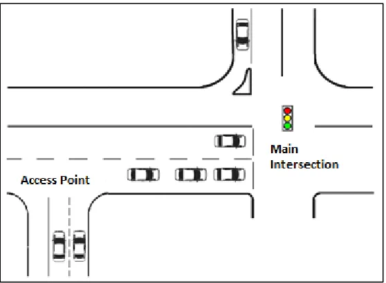
A question here is how the functional area can be specified. It’s also important to find out how far downstream and upstream access points can be located from an intersection. Figure 2 shows an upstream access point near a signalized intersection.
Figure 2 – Driveway upstream of a signalized intersection
2.2 Access management
Streets and highways are valuable and their safe operation requires appropriate access
8
to move smoothly and safely and residents and business owners have a right to access the roads. Thus the need for AM is essential as a balance between access and mobility. Prohibiting left turns, channelization, and other appropriate techniques significantly decrease access point crashes (8).
Researchers have been working on different techniques of access management (AM) for more than 30 years. An early classification of AM techniques was introduced by Stover et al. (9) in 1970. This was improved by Glennon et al. in 1975 (10). They provided checklists for the control of direct access to major roads and classified access techniques according to a) highway design and operation, b) driveway location, and c) driveway design and operation. In 1982, Flora (11) classified AM techniques by the following functional objectives: a) limit number of conflict points, b) separate basic conflict points, c) limit deceleration requirements, and d) remove turning vehicles from through lanes. In 1992, Koepke et al. (12) described different policy, planning, and design approaches to AM in various categories such as interchanges, frontage roads, medians, left turns, right turns; and driveway arrangements.
Bellomo-McGee (13) in 1993 included management elements with the access techniques and grouped the AM techniques as a) management, b) facility design, c) access driveway/design, and d) traffic control elements. NCHRP Report 420 in 1999, by Gluck et al., (3) emphasized policy (strategic) and design/operation (tactical) decisions in providing access to properties. They investigated safety, operation, environmental impacts, and economic impacts of the techniques such as intersections spacing, speed, corner clearance, median type, left turn lanes, U-turns, alternatives to direct left turns, and access separation. McCoy (14) and McCoy and Heimann (15) evaluated operational and safety impacts of driveway traffic volume on saturation flow rates at two signalized intersections. They found that driveway traffic can reduce the saturation flow rate on signalized intersection approaches. The amount of this reduction was found to depend on the corner clearance of the driveway and the proportions of volume that enter and exit the driveway.
9
1. Provide a specialized roadway system – it is important to design and manage roadways according to the primary functions that they are expected to serve;
2. Limit direct access to major roadways – roadways that serve higher volumes of regional through traffic need more access control to preserve their traffic function;
3. Promote intersection hierarchy – an efficient transportation network provides appropriate transitions from one classification of roadway to another;
4. Locate signals to favor through movements – long, uniform spacing of intersections and signals on major roadways enhances the ability to coordinate signals and ensure continuous movement of traffic at the desired speed;
5. Preserve the functional area of intersections and interchanges – the functional area is where motorists are responding to the intersection (i.e., decelerating, maneuvering into the appropriate lane to stop or complete a turn);
6. Limit the number of conflict points – drivers make more mistakes and are more likely to have collisions when they are presented with the complex driving situations created by numerous conflicts. Traffic conflicts occur when the paths of vehicles intersect and may involve merging, diverging, stopping, weaving, or crossing movements;
7. Separate conflict areas – drivers need sufficient time to address one potential set of conflicts before facing another;
8. Remove turning vehicles from through-traffic lanes – turning lanes allow drivers to decelerate gradually out of the through lane and wait in a protected area for an opportunity to complete a turn, thereby reducing the severity and duration of conflict between turning vehicles and through traffic;
9. Use non traversable medians to manage turn movements – they minimize left turns or reduce driver workload and can be especially effective in improving roadway safety; and
10. Provide a supporting street and circulation system – a supporting network of local and
collector streets accommodates development and unifies property access and circulation systems. Interconnected streets provide alternate routes for bicyclists, pedestrians, and drivers.
The Pennsylvania AM Handbook (16) summarizes the benefits of a good AM as follows:
Community and neighborhoods:
10
More attractive roadway corridors
Lower taxes for future roadway investment
Preservation of property values
Safer pedestrian and bicycle travel
Improved appearance of the built environment
Reduced fuel consumption and air emissions
Business community:
Stable property values
More consistent development environment
Reduced transportation and delivery costs
Pedestrians:
Safer walking routes due to fewer conflicts with traffic
Refuge areas created by medians
Bicyclists:
Fewer conflicts with traffic
More predictable traffic patterns
Greater choice of alternative travel routes
Transit riders:
Reduced delay and travel times
Safer walking environment for access to stations
Motorists:
Fewer traffic conflicts which increases driver safety
Fewer traffic delays
Governmental agencies:
Lower cost of providing a safe and efficient roadway
Improved internal and intergovernmental coordination
More success in accomplishing transportation goals
11 2.3 Corner clearance
Corner clearance is the distance between an intersection and the next driveway. The recommended corner clearance varies by state. Some of the states such as Florida provide different standards for different circumstances. Other states like Pennsylvania and North Carolina simply define a standard value regardless of the various circumstances.
The Florida Driveway Handbook (17) specifies the corner clearance based on access class and the roadway speed limit as shown in Table 1.
Table 1 – Florida’s corner clearance standards (17)
Access class Speed 45 mph Speed 45 mph 1 N/A - freeway N/A - freeway
2 1,320 660
3 660 440
4 660 440
5 440 245
6 440 245
7 125 125
This corner clearance could vary with the radius of the corner on the minor road as shown in Figure 3.
Figure 3 – Corner clearance and radius of the corner on minor street (17)
12
corner clearance should be at least 100 ft from the point of tangency of the curb curvature of the intersecting streets and no distance less than 50 ft is allowed. This distance for a full movement driveway next to a signalized intersection should be more than 100 ft. Per Mr. James Dunlop, the North Carolina Congestion Management Engineer, “The district engineers evaluate each permit individually, however developers have mostly learned that the closer to an intersection, the less likely full movement access will be granted. If a parcel's frontage is only 100', we cannot deny a driveway connection, however we can restrict it to right-in/ right-out (RIRO). If the parcel has direct access to another state road, we can restrict access to that other road in some situations”.
2.4 Collision models
Collision prediction models show the relation between the dependent variable of the number of collisions and the independent variables like the roadway speed, number of lanes, and other factors. Collision models usually are provided based on the historical data from the same or similar roadways. A simple linear form of the model, assuming a normal probability distribution of collisions is:
∑ (Equation 1)
Where,
is the expected number of crashes at the th segment, is the th variable at the th segment, and
is the th regression coefficient,
are the regression coefficients that need to be estimated .
13
In a Poisson distribution it is assumed that the variance of the number of collisions at the segment i is the same as the mean value at this segment. The relation between expected number of collisions and the variables is expressed as:
( ) ∑ (Equation 2)
Where () is the natural logarithm of the expected number of collisions and the Poisson model is:
( ) [ ( )( ) ] (Equation 3)
Where ( )is the probability of collisions at the th segment. If the variance of a collision
data set exceeds the mean value of this data, it’s said that the data are overdispersed. In this case, the variance won’t be the same as the mean, like the Poisson model. The negative binomial distribution is an alternative to treat the overdispersion problem by adding a quadratic term to the variance representing overdispersion. The relationship between the expected number of crashes at the segment and the variables is the same as for Poisson model but the negative binomial model is:
( ) ( ) ( ) (
) ( ) (Equation 4)
Where, ( ) is the probability of the collisions at the segment i and is the dispersion
parameter. The variance is . As → , the variance will be the same as the mean and
so the negative binomial model becomes the Poisson model.
14
Apparently one of the first safety collision models was developed by McDonald in 1966 (22). He developed a model to relate crash frequency to traffic flows at divided highway intersections. His model is shown as:
(Equation 5)
Where N was the number of crashes per year and and were major road and cross-road
ADTs.
In 1986 Persaud (23) and Lovell et al. (24) used traffic control type as an explanatory variable in their intersection crash models. They showed that the safety effect of converting to all-way stop was contradictory. Lovell and Hauer affirmed the benefit of converting to four-way stop, while Persaud rejected its effectiveness.
In 1975 King et al. (25) concluded that signalization reduces right-angle crashes but increases rear-end crashes, with no significant change in total crashes – related disutility. Lau and May (26,27) in 1988 and 1989, and Naclerio et al. (28) in 1989 looked at crashes at signalized and unsignalized intersections. These models were developed to identify locations where collision experience was more frequent or more severe than normal, and to evaluate the safety
consequences of alternative improvements. Three types of crash severity were modeled separately: fatal, injury, and property damage only. They used a nonparametric statistical modeling method known as the Classification Regression Tree. This method has particular applicability to categorical and discontinuous variables.
15
In 1995, Fridstrom et al. (30) developed a statistical model to predict collisions using traffic flow, climate, lighting condition, and speed limit. They considered negative binomial regression and a new methodology for goodness-of-fit measures.
In the same year Hadi et al. (31) proposed several collision prediction models for multilane roads and two-lane roads. They used Poisson and negative binomial regression models and related crashes to AADT and road environmental factors.
In 2000, Abdel-Aty et al. (32) developed a statistical model using the negative binomial distribution and related the collisions to AADT, degree of horizontal curvature, section length, lane, shoulder width, median widths, driver sex, driver age, and urban/rural designation.
In 2003 Golob et al. (33) used both linear and non-linear multivariate statistical analysis to relate collisions to traffic flow, weather, and lighting conditions. Continuing this research in 2004 they developed another model using crash type, location, and severity (34).
In 2004 Hauer et al. used a negative a multinomial likelihood distribution for collision counts to model them on urban four-lane undivided roads (35). In another effort Hauer (36) presented a derivation of the negative multinomial likelihood function for collision models. He used a ratio of recorded collisions and collisions predicted by the current model. The introduced variable was first grouped into bins and then the ratios were calculated for each bin. This identifies the
16
( ) ( ) ( ) (Equation 6)
Where is the estimated number of collisions, are the variables, and () () ()
are the functions of the variables to be estimated.
17
3.
D
ATA PREPARATIONI used historical data from a 5-year monitoring period extending from January 2005 to December 2009 to develop a statistical collision prediction model. To obtain proper data I first chose the appropriate study locations and then collected geometry, traffic, and crash data. In the end, to choose an accurate modeling method the collected data was analyzed. Figure 4 illustrates the tasks performed to prepare data for this research.
Data Collection
Section 3.2
Site Selection
Section 3.1
Geometric Data
Section 3.2.1
Traffic Data
Section 3.2.2
Collision Data
Section 3.2.3
Data Analysis
Section 3.3
Data Preparation
Chapter 3
Figure 4 – Data preparation overview
3.1 Site selection
18
are built and maintained to the same standards. Therefore Wake County is a good representative of North Carolina counties and was chose for data collection. Figure 5 illustrates Wake County among the other North Carolina counties.
Figure 5 – Wake County in the State of North Carolina (38)
For the purpose of this research a few criteria were taken into account for site selection. The criteria are listed and described in details below.
1- Random selections: Collection of an unbiased and random subset of the data is a key process to yield collision predictions. Each one of the 739 signalized intersections in Wake County was assigned a random number. Then these random numbers were sorted and the first 200 signalized intersections were chosen. For this study a site was defined as a leg of the intersection that fulfills the minimum requirements as described below. Each intersection may consist of 3, 4, or 5 sites depending on the number of the legs at the intersection. The 200 signalized intersections consisted of 674 sites. This means most of the intersections had 4 legs.
19
3- Access points upstream of the intersections: Driver behavior, signing, and other factors depend on whether an access point is upstream or downstream of the intersection. At the upstream access point, as shown in Figure 2, drivers approaching the intersection should be aware of the traffic leaving or entering the access point. I decided to focus on these upstream access points as their issues are more serious than the downstream access points, in that the intersection queue may back up and block or limit the access point movements.
4- No free flow right movement at the intersection: One of the reasons that the researcher decided to study the access points near intersections is the queue back up. In case of a free flow right turn, queues may not form and the issue of the access point being next to the intersection wouldn't be as interesting. Thus for site selection I decided to focus on sites with no free flow right turn. Figure 6 illustrates regular and free flow right turns.
Figure 6 – (A) Signalized right turn, (B) Free flow right movement
5- Closest access point to the intersection: Many driveway issues are the ones near intersections, so the researcher decided to focus on the closest access point upstream of the intersection.
20
7- Major roads grades less than 4%: Usually operational and safety problems increase on intersection approaches with grades of 4% or higher. Because of these negative impacts, and since in Wake County most of the roads are in flat terrain, I decided to concentrate on roads with grades of less than 4%.
All the sites in the sample of 200 intersections were scanned and filtered by implementing the above limitations. Table 2 lists all the lane configurations at the driveway (LCD) in the sample of intersections that emerged after I applied the seven criteria listed above. Up to this point I had 37 configurations at the driveway and a total of 260 sites.
Table 2 – Lane configurations at the driveway (LCD)
Site 6 1 3 1 4 3 2 9
LCD
Sites 1 1 2 1 3 10 2 1
LCD
Site 3 2 36 16 11 10 2 1
LCD
Site 12 6 2 5 31 11 26 1
LCD
Site 1 5 9 13 7
LCD
21
8- No more than two through lanes at the access point: Operations at the access point would be much more complicated when vehicles exiting the access point needed to cross more than two lanes to be positioned at the desired direction. In the other hand, as shown in Table 2, the number of sites with configurations of more than two through lanes is small compared to the sites with two through lanes and would therefore be hard to model statistically. As a result the researcher decided to scope the research down to sites with one or two through lanes at the access point.
9- No driveway associated with a different parcel within 150 ft of the main access point: If a different parcel has a driveway within 150 ft from the main access point, this site was eliminated from the candidate site list. Operation and safety issues at the second access point would
significantly affect the first access point in ways that cannot be documented properly. In particular, collisions could not be attributed to the correct access point. For the cases when one parcel has a second access point within 150 ft from the first one, a variable will be introduced to distinguish them from the other sites, as discussed later.
10- Lane configurations at the driveway with 10 sites or more: Results from the statistical modeling might be unconvincing if the number of sites of each type was not sufficient. For the purpose of this research I decided to model the lane configurations at the driveway with 10 sites or more as shown later in Table 3.
11- Four-leg signalized intersections: I noticed that less than 5% of the study intersections surviving to this point had three legs and no intersections had more than four legs. Thus, the researcher focused on only four-legged intersections.
12- No sites with geometry changes within the last 5 years: Since the collision data were to be collected for a period of 5 years starting January 2005, sites with any geometry changes at or near the access point were eliminated. This is because the collision data should be unbiased from any external change or revisions.
22
Because of these complications, sharply-curved and odd geometry sites were eliminated from the site list. There were only a few cases with these characteristics.
14- Only public (state or city) owned roads: Some law enforcement agencies report the crashes only on public-owned roads. Also non-public roads, such as private roads in shopping centers, are not of much policy interest. As a result if the main study roadway was a private road, such as an entrance to a shopping center, it was eliminated from the database.
15- No small driveways: A site was not considered for data collection if its access point was unpaved or it served only a single-unit residence. The low traffic volumes of these access points provide only a slight risk of causing a collision.
16- Driveway movement type: The median type at the access point on the major road guide the drivers how and where to drive. Channelization, signing, and pavement marking help the them to understand the roadway configuration and follow the rules. Full movement, left-over (directional cross-over), and RIRO are the main three types of driveways, with the latter two designs being generally more desirable from a safety point of view where an access point is located within the functional area of an intersection. Figure 7 illustrates full movement, left-over, and RIRO designs.
Figure 7 – Full movement, left-over, and RIRO designs
23
down to only full movement and RIRO sites and delete the site with left-over design from the list. After applying above criteria, 103 sites were left in the study list.
The next chapter will discuss in detail how I collected the collision data. After a careful review of the sites’ collisions it came to my attention that only 4 out of the 103 sites have relatively higher collision frequencies with 15, 16, 21, and 32 crashes over the study’s 5 years. The rest of the sites had less than 7 collisions over the studied 5 years. As a result I decided to look further and find a few more sites with high number of crashes. I scanned the sites in Wake County randomly again and found 10 sites with some recent median changes at access points that meet all criteria discussed previously. The reason behind this step is that I presumed the improvements to the median took place because of complaints received by residents or investigations done by traffic engineers as a result of the high collisions at those sites. Indeed 5 of these 10 sites were already considered in our study but the crash data between 2005 and 2009 applied to the time when the median was already in place. Now I collected 5-year crash data from before any countermeasures were implemented at the site. The other 5 sites were thereby added to the sample. As a result the ultimate number of sites was 108. These sites are near 63 signalized intersections. A pin map of these 108 sites distributed in Wake County is shown in Appendix A. Table 3 shows the lane configuration of these 108 sites at their driveways.
Table 3 – Sites lane configuration at the driveway
Configuration I II III IV V VI
Type of Configuration
Number of Sites 23 10 32 12 20 11
24 3.2 Data collection
A complete set of data, including geometric, traffic, and crash data, were needed to statistically model the collisions at the access points.
3.2.1 Geometric data
I collected data on all geometric factors that I thought might affect the crash rate of interest at the sites in the sample. These factors included:
Corner clearance (CC), i.e., the distance between closest driveway and the intersection
Lane configuration at the driveway on the major road (LCD)
Lane configuration at the intersection near the access point on the major road (LCI)
Major road median type at the access point (MM)
Speed limit on the major road (SL)
Grade on the major road (GR)
Driveway angle, i.e., the angle between driveway centerline and the edge of travel way (DA)
Driveway one-way or two-way operations
Exclusive right turn into driveway
Driveway median status, i.e., divided or undivided driveway (DM)
Driveway width (DW)
Transition between major road and driveway pavements (TR)
Driveway radius (RA)
Existence of another second driveway associated with the same parcel within 150 ft from the
main access point (AD)
25 3.2.2 Traffic data
The most important explanatory variable in a statistical collision prediction model is usually traffic volume. Traffic volume represents the amount of exposure to the risk of collision. The traffic volume used for the purpose of this research consisted of the major road traffic volume and the access point traffic volume. The queue backed up at the intersection near the access point was also an estimated data using Synchro software. The methods to collect and estimate these data are described below.
3.2.2.1 Major road traffic volume
For major road traffic volumes, the Traffic Survey Group of the NCDOT provides
comprehensive AADT data for the major road segments in North Carolina. The AADT database is presented in the form of map sheets on which road AADTs are spotted manually. Figure 8 illustrates a snapshot of the AADT map adjacent to NC State University.
Figure 8 – A snapshot of the AADT map (39)
26
Google Earth Pro, Version 5.2.1, added a new feature called “US Daily Traffic Counts”. This feature shows the AADTs for some of the major roads in the US as illustrated in Appendix B. I obtained some of the missing AADTs from Google Earth Pro.
Since the NCDOT information was included in the Google Earth Pro, I validated accuracy of the Google Earth Pro data by comparing them with the NCDOT AADT Maps for over 20 cases. The collected AADT values were almost the same.
In the few cases that the AADT map and Google Earth Pro did not provide the needed AADT, traffic data for the nearest point was assumed to be the same as for the study segment. For a few other cases, where there was no traffic volume available on or near the road segment, the missing data were interpolated by two AADTs located on either side of the road segment. If none of these techniques was helpful to find the AADT, the AADT was estimated using traffic counts obtained from the city engineer or collected manually. The traffic counts were converted to an AADT using Equation 7:
(Equation 7)
Where is the proportion of AADT occurring in the hours counted and is the seasonal
27
Table 4 – K factors (40)
The seasonal factor is used to adjust a daily volume count to AADT estimate. The NCDOT provides the seasonal factor for different types of roads. Table 5 illustrates these values for the types of roads in our research per month and day of the week based on the date the data were collected. If the manual count were collected on two different days, I used an average weekday factor for the month counted.
Table 5 – Seasonal factors (40)
Hour Interstate US NC SR Local
12:00AM 0.0110 0.0064 0.0063 0.0068 0.0068
1:00AM 0.0081 0.0040 0.0039 0.0037 0.0037
2:00AM 0.0071 0.0033 0.0032 0.0029 0.0029
3:00AM 0.0073 0.0036 0.0035 0.0027 0.0027
4:00AM 0.0098 0.0064 0.0071 0.0047 0.0047
5:00AM 0.0192 0.0183 0.0189 0.0149 0.0149
6:00AM 0.0439 0.0441 0.0447 0.0396 0.0396
7:00AM 0.0664 0.0695 0.0721 0.0780 0.0780
8:00AM 0.0595 0.0589 0.0595 0.0581 0.0581
9:00AM 0.0530 0.0535 0.0528 0.0474 0.0474
10:00AM 0.0534 0.0547 0.0534 0.0472 0.0472
11:00AM 0.0553 0.0578 0.0589 0.0545 0.0545
12:00PM 0.0569 0.0607 0.0631 0.0612 0.0612
1:00PM 0.0593 0.0619 0.0612 0.0606 0.0606
2:00PM 0.0638 0.0668 0.0681 0.0668 0.0668
3:00PM 0.0701 0.0751 0.0757 0.0747 0.0747
4:00PM 0.0743 0.0809 0.0809 0.0801 0.0801
5:00PM 0.0749 0.0820 0.0807 0.0832 0.0832
6:00PM 0.0577 0.0600 0.0580 0.0630 0.0630
7:00PM 0.0432 0.0419 0.0409 0.0480 0.0480
8:00PM 0.0348 0.0328 0.0319 0.0382 0.0382
9:00PM 0.0298 0.0263 0.0254 0.0300 0.0300
10:00PM 0.0234 0.0187 0.0181 0.0200 0.0200
11:00PM 0.0175 0.0125 0.0120 0.0138 0.0138
24-Hour 1.0000 1.0000 1.0000 1.0000 1.0000
28 3.2.2.2 Access point traffic volume
The AM and PM peak hour traffic volumes entering and exiting the access point are one of the key independent variables. I used the following techniques to collect or estimate these volumes.
Some of the access points are unsignalized intersections of the major road and a minor road. Peak hour turning movement counts for these intersections were obtained from the city engineer or collected manually on site or in the office. A camera was used to record the events as shown in Appendix C.
If the access point was associated with a residential subdivision, or a small parcel such as a gas station, convenience store, or fast food restaurant, the square footage of the buildings were derived from the Wake County GIS website or the Google Earth Pro tool (US Parcel Data). Then the Trip Generation Manual (41) was used to estimate the peak hour traffic volumes entering and exiting the access point. The higher peak hour volume was chosen among the AM and PM peak hours.
Multi-use development is defined by ITE as a single real estate project that consists of two or more ITE land-use classifications between which trips can be made without using the off-site road system. For the multi-use land developments, the trip generation process could be more complicated because the Trip Generation Manual would likely over-estimate the generated trips due to the internal circulating traffic and activities between on-site land uses.
29
While reviewing the aerial historical images and visiting the study site areas if I noticed an empty parking lot during regular business hours, that particular land use was assumed to be vacant. Exceptions were made for some business with time-limited activities such as churches.
For subdivisions with multiple access points the typical methodology used for traffic impact analysis (TIA) was implemented for trip distribution. The geographic position of each access point and adjacent road led the analyst to come up with a reasonable assumption of the percentage of produced and attracted traffic that would use each access point. If such an
assumption was not reasonable, I assumed that each access point was used proportionally to the adjacent road’s AADT.
3.2.2.3 Queue at the intersection near the access point
Queue length was estimated using the Synchro software because it was more convenient than actual site data collection and queue observation and because it has been widely used by analysts in traffic engineering for the last few years. The available turning movement and signal timing information were used as inputs to Synchro to obtain the estimated 95% queue, in feet at the intersection near the access point. The 95% queue in Synchro is the maximum back of queue
with 95percentile traffic volume (44).
30
Figure 9 – Queue on Oneal Road in Raleigh, NC
3.2.2.3.1 Queue validation
31
Table 6 – Observed and Synchro estimated maximum queue values Observed queue (#cars) Observed queue (ft) Estimated queue (ft)
3 75 149
11 275 394
1 25 87
14 350 523
8 200 224
3 75 123
7 175 121
11 275 325
9 225 377
19 475 638
5 125 219
6 150 89
5 125 157
14 350 541
Mean 207 283
These values are plotted in Figure 10 to compare the Synchro estimated and observed queues.
Figure 10 – Synchro estimated queue versus observed queue
A regression analysis shows a linear relation between queues with a slope of 1.37 and standard error of 0.144. This means if an analyst collects the maximum queue at the intersection, this value can be multiplied by 1.37 to be usable by this research prediction model. In the other
y = 1.37x R² = 0.88
Ideal regression: y = x
0 100 200 300 400 500 600 700
0 100 200 300 400 500 600 700
Sy n ch ro E sti ma ted Q u eue ( ft)
32
words, on average the Synchro estimated queue lengths are 37% higher than the observed maximum queues. This different could be because:
The definition of 95% queue in Synchro is the maximum back of queue with 95th percentile
traffic volume while the maximum queue observed was derived from the maximum of the vehicles waiting at the intersection during the peak hour traffic volume.
I considered an average of 25 feet between bumper to bumper of the vehicles but this value
could be different depending on the number of trucks and other vehicles.
Synchro estimation was using the available signal timing plans’ information. These could
have been changed when the observed maximum number of vehicles was collected.
3.2.3 Collision data
Collisions reported on any roadway in North Carolina can be obtained from the collision
database Traffic Engineering Accident Analysis System (TEAAS). In case a road has more than one road name, reported collisions can refer to different road names, so it was important to obtain all roadway names.
To develop a statistical model I collected 5 years of collision reported data, from January 2005 to December 2009. Law enforcement agencies are not required to submit non-reportable crashes and as a result these collisions are not included in our research. The reportable crashes must meet at least one of these criteria: a) results in a fatality, b) results in a non-fatal personal injury, c) results in property damage of $1,000 or greater, or d) results in property damage of any amount to a vehicle seized. A seized vehicle is a vehicle involving alcohol or other drugs in sufficient amount to constitute a DWI, a stolen, repossessed, or with other such history. The reportable crashes must also occur on public roadways. A copy of the North Carolina Police report is shown in Appendix D. Collisions were collected on both side of the major road on a full
movement access point, but for the RIRO design only the collisions on the side of the driveway location were collected.
33
limited to those outside the physical area of the intersection. The physical area was shown in Figure 1.
3.2.3.1 Obtaining individual collision IDs and collision reports
To obtain the actual police reports from NC DMV website, each individual collision ID was needed. TEAAS was used to find the collision IDs near the intersections. The following steps were followed to make sure all the collisions were reviewed and no useful collision data were missed.
1- Coinciding names: As mentioned earlier, some of the roads have one or more coinciding names or local city names. Depending on the police officer notes, TEAAS provides crash IDs to different collisions for each one of the names. For example, the segment of Capital Boulevard between I-440 and New Hope Church/ Buffalo Road is also known as US-1, US-401, and SR-2179. Using different methods such as a feature in TEAAS called "Feature Names, Secondary Routes and Exceptions", Google Earth Pro images, and site visits I identified what I hope are all the possible route names for the sample segments.
2- 1000 ft from the intersection: As mentioned earlier, access points within 800 ft upstream of the intersection are in the feasible study area of this research. On the other hand collisions within 150 ft away from the access point were considered for modeling. The researcher used a feature of TEAAS called "Intersection Analysis Report" for the period of 5 years to extract the reported crashes. To avoid missing any useful data, all the collision data up to 1000 ft away from the intersection were collected.
34
Figure 11 – A snapshot of a police report diagram and narrative
A complete list of the collected collisions IDs is presented in Appendix E.
3.2.3.2 Filtering the collision reports
Since access – related collisions are of the interest of this study, first all the crashes within 150 ft from the access point were considered and then I filtered them down to the ones related to the access point within the said distance. To collect the access – related collisions it was essential to derive a logical set of criteria to distinguish the crashes that occurred because of the existence of the access point. One of the indications listed in the police report (number 49) states the vehicle maneuver/ action. This field states if the vehicles are making right turn, left turn, U turn,
slowing, parking, etc. and helped the researcher in finding the access point – related crashes. A collision needed to satisfy at least one of the criteria below to be included in the access – related collision analysis.
The narrative or diagram of the collision indicated that at least one of the vehicles involving
the collision is clearly headed to or from the driveway, or
Any word like "driveway" or "access point" is in the narrative section of the police report, or
Field number 49 of the police report (shown in Appendix D) stated that one of the vehicles
35
The criteria that were followed to delete collisions from the analysis were:
Collisions involving pedestrian or animal
Collisions involving vehicles travelling on different major intersection approaches, or
Collisions that happened in the physical area of the intersection (as shown in Figure 1).
3.3 Data analysis
This section describes the collected geometry data qualitatively and quantitatively.
3.3.1 Corner clearance
The distance between the closest driveway and the intersection is defined as corner clearance and is measured from the curb’s intersecting tangent lines at the intersection to the curb’s tangent lines at the access point. These data were collected for all eligible intersections and are illustrated in Figure 12.
36
Figure 12 shows that the distribution of corner clearances covers a wide range of distance. The database provides lots of small and large corner clearances that should help calibrate a
reasonable model for this variable.
The North Carolina Driveway Manual (6) defines the corner clearance as "at an intersecting street or highway, the distance measured from the edge of the pavement curb line or the intersection of the right of-way lines to the beginning of outside driveway radius". This
definition is different from what was used in this research. Figure 13 illustrates these two corner clearance measurements with “CC” representing the corner clearance.
Figure 13 – Corner clearance measurements
On average, corner clearance measured according to the NCDOT Driveway Manual is 65 ft less than the measurement in this research.
3.3.2 Lane configuration at the driveway
The lane configurations on the major road at the driveway were shown in Table 3. As discussed earlier, I decided to collect the data for 6 major categories of the lane configurations at the driveways.
3.3.3 Lane configuration at the intersection
37
Table 7 – Lane configuration at the intersection
LCI* category
LCI* shape Frequency
1 L,T,TR 42
2 L,TR 25
3 L,T,R 17
4 LT,R 11
5 L,T,T,R 10
6 L,L,T,R 2
7 L,L,TR 1
Total 108
* LCI: Lane configuration at the intersection
In the table "L", "T", and "R" are left, through, and right lanes, respectively. "LT" is a left and through shared lane while "TR" refers to a through and right shared lane.
3.3.4 Major road median type
As mentioned earlier, the only left-over site was eliminated from the sample. Table 8 shows the number of full movement and RIRO sites.
Table 8 – Full movements and RIRO sites
Median type Frequency
Full Movement 77
RIRO 31
Total 108
3.3.5 Speed limit on the major road
Major road speed limit was considered as one of the variables in the collision model. Out of 108 eligible sites, one site is operating with no posted speed limit which implies 35 miles per hour
(mph). Table 9 shows the posted limit in mph for the sample. Forty-eight percent of the sample
38
Table 9 – Posted speed limit on the major roads
Speed limit (mph) Frequency
15 1
20 0
25 8
30 0
35 42
40 0
45 53
50 0
55 3
No Posted Speed Limit 1
Total 108
3.3.6 Grade on the major road
Steep roads have negative impacts on operations and safety. Usually these issues occur at intersection approach grades 4% or higher. Since most of the roads in Wake County are in flat terrain I decided to study the roads with grades of less than 4% and delete the steeper sites. There was only one site with a grade of 0.5. To ease the analysis this site assumed to be flat. Table 10 shows grades of all sample sites at the access point.
Table 10 – Major roads grade at the access point
Major road grade (percent) Frequency
-3 12
-2 18
-1 15
0 12
1 17
2 26
3 8
Total 108
3.3.7 Driveway angle
39
Figure 14 – Driveway angle
Table 11 lists the driveway angles for the sample sites. Almost 68% of the sites have a right angle.
Table 11 – Driveway angle
Driveway angle (degrees) Frequency
50-59 1
60-69 1
70-79 8
80-89 2
90-99 73
100-109 7
110-119 9
120-129 6
130-139 1
Total 108
40
Figure 15 – Short driveway stem
For these cases, it was assumed that the vehicles' moving direction on the driveway would be perpendicular to the major road and as a result a 90-degree angle was recorded.
3.3.8 Driveway one-way or two-way operations
Initially I expected that some of the driveways may be restricted to one-way only. After
examining the sites in the sample it appeared that all driveways are operating in two directions. As a result this variable was not used in model calibration.
3.3.9 Exclusive right turn into driveway
I was expecting some of the access points to have exclusive right turn lanes on the major road entering into the driveway. However, none of the studied sites provided an exclusive right turn lane. Therefore, this variable was also deleted from the list.
3.3.10 Driveway median status