Underwater Free Space Optics

(1)

ABSTRACT

GAWDI, YASH JAGDISHLAL. Underwater Free Space Optics.(Under the direction of Dr. John F. Muth and Dr. Leda M. Lunardi.)

Radio waves propagate poorly in water and acoustics have been the dominant method for undersea communications, but its data rates are bandwidth limited. Free Space Optics potentially provides an alternative solution to acoustical communications with wider bandwidth and wireless flexibility that would benefit many undersea applications over short ranges.

(2)

UNDERWATER FREE SPACE OPTICS

by

YASH JAGDISHLAL GAWDI

A thesis submitted to the

Graduate Faculty of North Carolina State University in partial fulfillment of the requirements for the

Degree of Master of Science

ELECTRICAL AND COMPUTER ENGINEERING

Raleigh, North Carolina 2006

APPROVED BY:

___________________________

__________________________

Dr. John F. Muth Dr. Leda M. Lunardi

(Chair of Advisory Committee) (Co-Chair of Advisory Committee)

________________________________ Dr. Kevin G. Gard

(3)

I would like to dedicate my Thesis to

my parents (Mr. Jagdish and Pushpa Gawdi),

my sister & brother-in-law (Dr. Meghna and Dr. Divyagynan Sarvaiya),

(4)

BIOGRAPHY

The author was born in Bombay, India on the 10th of August 1982. He earned his Bachelors degree in Electronics Engineering from Mumbai University, India in May 2004. He had the privilege of working with Global Telesystems Ltd., India for his final year project, where he assisted as a link engineer to design and commission a point to point Microwave link. He has been a Masters student at North Carolina State University, USA in the department of Electrical and Computer Engineering since August 2004. He was honored with the position of a Research Assistant under Dr. John Muth and Dr. Leda Lunardi. He has held the position as a Teachers Assistant for Dr. John Muth and Dr. Michael Escuti in Photonics and Optical communication. His interests lie in RF & Microwave circuit design and optical communication.

(5)

ACKNOWLEDGEMENTS

Foremost, I would like to thank Dr. John Muth for giving me an opportunity to work under him and be a part of his research group. This research is a result of his vision and guidance. I would like to convey my sincere gratitude to Dr. Leda Lunardi for her continuous encouragement and help through out my research. She has been very patient and instrumental during the preparation of this thesis. I would like to acknowledge Dr Kevin Gard for establishing my foundations in subjects like analog circuits and being a part of my advisory committee.

Special thanks to Dr. Dan Kamykowski (Marine, Earth & Atmospheric Sciences), Geoffrey Sinclair and Blake Schaeffer for sharing their facility and information which was very helpful in my research. I would like to acknowledge National Science Foundation for providing the funds to carry out this research.

I would like to show my appreciation to all the students of my research group, especially Khalid Alhamadi, Anuj Dhawan and Praveen Golakotta for all their help during the past year.

I am thankful to Harnish, Siddharth for being great friends and for supporting me selflessly through my two years at NC State. I appreciate the good time that I have spent with my friends Arin, Ullas, Mitul, Aditya, Ira, Viraj, Manan and Harshwardhan. I am thankful to my friend Mrunal, my sister Meghna and my fiancé Vijeta for being the pillars of support throughout my life.

(6)

LIST OF TABLES

(9)

LIST OF FIGURES

Figure 1-1 Spectral attenuation coefficient of ocean waters ... 1

Figure 2-1 Geometry used to define inherent optical properties ... 5

Figure 2-2 The Absorption coefficient of pure sea water... 8

Figure 2-3 Cubic spline curve fit for spectral absorption coefficient of chlorophyll-a ... 9

Figure 2-4 Cubic spline curve fit for the specific absorption coefficients of chlorophyll-b, chlorophyll-c, carotenoids pigments... 10

Figure 2-5 Spectral absorption by CDOM ... 11

Figure 2-6 Scattering coefficient of Pure Seawater ... 14

Figure 2-8 Volume scattering function measured for coastal ocean at =514nm. ... 15

Figure 2-9 Spectral scattering coefficients of large and small particles for seawater with 1mg/m3 _{of chlorophyll concentration... 16}

Figure 2-10 Variation in the refractive index of sea water with change in wavelength .. 18

Figure 2-11 Variation in the refractive index of sea water with change in the temperature.. ... 18

Figure 2-12 Variation in the refractive index of sea water with change in the salinity... 19

Figure 2-13 Variation in the refractive index of sea water with change in pressure... 19

Figure 3-1 Satellite remote-sensing of Chlorophyll-a concentration... 23

Figure 3-2 Absorption in sea water with 1mg/m3 of Chlorophyll concentration. ... 26

Figure 3-3 Various constituents of scattering coefficient... 28

Figure 3-4 Total absorption and scattering coefficients ... 29

Figure 3-5 Vertical distribution profiles of chlorophyll ... 32

Figure 3-6 Vertical distribution model of chlorophyll ... 33

Figure 3-7 Procedure for estimating five parameters of the chlorophyll vertical profile from surface chlorophyll concentration... 34

Figure 3-8 Calculating the chlorophyll concentration between the source and receiver 35 Figure 3-9 Dividing the path length into intervals to calculate the chlorophyll concentration ... 36

Figure 4-1 Scattering observed in sea water using a Red He-Ne Laser ... 41

(10)

(11)

Figure 4-19(b) Side view and front view images of green laser beam spread for different

latex-acrylic paint concentrations and the corresponding intensity profiles ... 57

Figure 4-20 Beam attenuation vs. Depth for different chlorophyll concentrations using source operating at 532nm. ... 61

Figure 4-21(a) Wavelengths corresponding to minimum attenuation for different chlorophyll concentrations using MathCAD model. ... 63

Figure 4-21(b) Wavelengths corresponding to minimum attenuation for different chlorophyll concentrations using MathCAD model (zoomed region 400nm-600nm). ... 63

Figure 4-22 Percentage difference between Beer’s law and beam spread function for different concentrations of chlorophyll calculated using MathCAD... 65

Figure 4-23: Experimental setup for measuring attenuation in seawater... 66

Figure 4-24 (a) Comparison between the observed values and calculated values of beam attenuation for green laser (<5 mW)... 68

Figure 4-24 (b) Comparison between the observed values and calculated values of beam attenuation for red laser (1 mW) ... 69

Figure 4-25 Received power calculated using beam spread function for different concentrations of chlorophyll with 1 W source. ... 70

Figure 4-26 Received power calculated using beam spread function for different concentrations of chlorophyll with 100 mW source. ... 71

Figure 4-27 Four cases considered for link budget calculations... 72

Figure 4-28 Vertical chlorophyll distribution and five parameter curve fit for region 1. 73 Figure 4-29 Vertical chlorophyll distribution and five parameter curve fit for region 2. 74 Figure 4-30 Vertical chlorophyll distribution and five parameter curve fit for region 2. 76 Figure 4-31 Block diagram to calculate beam attenuation and the received power... 78

Figure 4-32 Graphical user interface to calculate the link equation ... 79

Figure 5-1 Diagram showing the larger spot than the field of view of the detector. ... 82

Figure 5-2 Geometry used to calculate the diameter of the spot size v/s. distance... 83

Figure 5-3 Spot sizes v/s. link range for lasers with divergence angles... 84

Figure 5-4 Beam Divergence and Antenna Gain comparison... 87

(12)

(13)

LIST OF ABBREVIATIONS

Abbreviation Full Description

APD Avalanche Photodiode

CDOM Color Dissolved Organic Material

FSO Free Space Optics

Gbps Giga bits per second kbps Kilo bits per second

LED Light Emitting Diode

LOS Line of Sight

nm Nano meters

pW Pico-Watts

RF Radio Frequency

(14)

LIST OF SYMBOLS

Symbol Unit Description

radians Angle of the path length from the vertical )

(λ

a m-1 Total spectral absorption coefficient

( )

λ

w

a m-1 Absorption coefficient for pure seawater

( )

λ cl

a m-1 Absorption coefficient for chlorophyll

( )

λ o c

a m-1 Specific absorption coefficient of

chlorophyll

( )

λ

f

a m-1 _{Absorption coefficient for fulvic acid}

( )

λ

o f

a m-1 Specific absorption coefficient of fulvic acid

( )

λ h

a m-1 _{Absorption coefficient for humic acid}

( )

λ o h

a m-1 Specific absorption coefficient of humic

acid c

C mg/m3 Total concentration of chlorophyll

f

C g/m3 Concentration of fulvic acid

h

C g/m3 Concentration of humic acid

( )

λ

b m-1 Total spectral scattering coefficient

( )

λ o

b m-1 Scattering coefficient of pure seawater

( )

λ o s

b m-1 Scattering coefficient of small particles

( )

λ o l

b m-1 Scattering coefficient of large particles

s

C g/m3 Concentration of small particles

l

C g/m3 Concentration of large particles

) (z

Chl_depth mg/m3 Chlorophyll concentration as function of depth

o

B mg/m3 _{Background chlorophyll concentration}

S mg/m3/m Vertical chlorophyll concentration gradient

z m Depth

h mg/m2 Total chlorophyll above the background

σ

unit less Standard deviation of Gaussian distribution

τ

seconds Multipath time delay

mean

(15)

Symbol Unit Description

max

z m Depth of chlorophyll maximum

r

P W Optical power received

Pt W Initial optical power from transmitter

r

D m Diameter of receiving aperture

t

D m Diameter of transmitting aperture

Div radians Divergence of the optical beam

Lm m Distance of optical link

(16)

CHAPTER 1 INTRODUCTION

Communication underwater is very challenging. Unlike terrestrial communication links, radio frequencies and microwaves do not propagate through water. Acoustics communication links have been of keen interest for underwater applications in the past few decades, but provide limited bandwidth [1]. Optical communication satisfies the requisites of high bandwidth, efficient and reliable links, but numerous undersea applications would benefit from the flexibility of wireless links. We investigate the application and feasibility of Free Space Optical links to serve the purpose of underwater communications. Free Space Optical modules can be potentially deployed on Unmanned Underwater Vehicles (UUV) that would provide an extra degree of freedom to communicate with fixed bases or other UUV’s. As seen in Figure 1-1, the blue-green region of the visible spectrum has the least attenuation. Communicating with floor sensors for data collection or adhoc networks would significantly enhance ocean laboratories. Remote inspection of oil rigs, real-time video transmission and communications between underwater platforms are other examples of underwater applications.

(17)

Terrestrial Free Space Optical links have demonstrated operational success for short links and can be used as a model for underwater communication links. However ocean waters offer high attenuation which is at least two orders higher than the worst atmospheric conditions. To better understand the problem, it is important to survey the system performance over wide spectrum of ocean waters types and sea state conditions.

The overview of the problem can begin with drawing parallels between optical fiber communication and free space optical communication. The basic difference between the two is the absence of a fiber channel in free space optics. For underwater applications the medium for free space optics is water. Ocean waters are a new medium for optical communication and hence it is important to understand the nature of light propagation through these waters; qualitatively and quantitatively. Ocean waters contain organic and inorganic materials that influence the absorption and scattering of light. The complexity of the problem increases as, the concentration of organic and inorganic not uniform and varies with the place and time. There needs to be a general model that takes into consideration these variations and to estimate the total light attenuation for different ocean conditions, since its essential to know the signal losses in the medium before designing a communication link. Separate models are present in oceanography that deal with individual parts of these sub-problems like, determining the concentration of organic particles in water, specific absorption and scattering coefficients of pure seawater and its constituents etc. But there is an absence of a general attenuation model that can be applied to most water types. This research investigates this problem from an optical communication point of view, estimating the unknown factor of signal attenuation.

Objectives:

• Provide systematic approach to the problem of light propagation in natural

waters, in the context of optical communications.

• Develop a general model that estimates the total attenuation in sea water that can

be made applicable to a variety of ocean conditions.

• Conduct experiments to enhance the understanding of the phenomena of

(18)

Chapter II introduces the optical properties of water and establishes the foundations of absorption and scattering by natural waters. The effects of absorption and scattering are distributed among the various constituents of water [3, 4].

Chapter III presents a one-parameter bio-optical model that defines the absorption coefficient and scattering coefficient of water. Based on empirical work, the constituents of ocean water can be correlated to the chlorophyll concentration [5]. Various methods to estimate the chlorophyll concentration are discussed. A model is developed in MathCAD that computes the total chlorophyll concentration in water and estimates the absorption and scattering coefficients.

Chapter IV examines the scattering phenomena. An empirical particulate scattering is carried out to qualitative understand the influence of scattering on the beam attenuation. A model is developed that calculates the total beam attenuation which is based on the multipath time delay caused due to scattering [6]. Being a different approach, this beam attenuation model is compared to Beer’s Law, which supported by an experiment of light transfer in seawater containing chlorophyll. MathCAD simulations are included that compute the total beam attenuation for different water types.

(19)

1.1 References

[1] I. F. Akyildiz, D. Pompili and T. Melodia, "Underwater acoustic sensor networks: research challenges," Ad Hoc Networks, vol. 3, pp. 257–279, 2005.

[2] M. E. Katzman, Laser Satellite Communications. New Jersey: Prentice Hall Inc., 1987, pp. 1-30.

[3] C. D. Mobley, Light and Water- Radiative Transfer in Natural Waters. California: Academic Press Inc., 1994, pp. 60-144;300-303;487-488.

[4] R. E. Walker, Marine Light Field Statistics. New York: John Wiley & Sons Inc., 1994, pp. 142-162;168-172.

[5] V. I. Haltrin, "Chlorophyll-based model of seawater optical properties," Applied

Optics, vol. 38, 1999.

[6] J. W. McLean, J. D. Freeman and R. E. Walker, "Beam spread function with time dispersion," Applied Optics, vol. 37, 1998.

[7] S. G. Lambert and W. Casey, Laser Communication in Space. MA: Artech House Inc., 1995, pp. 94-119.

[8] S. Bloom, E. Korevaar, J. Schuster and H. Willebrand, "Understanding the performance of free-space optics," Journal of Optical Networking, vol. 2, 2003.

(20)

CHAPTER 2 OPTICAL PROPERTIES OF WATER

2.1 Introduction:

In order to estimate the attenuation of light, we need to understand the nature of the optical properties of the medium. Optical properties of natural waters are very different as compared to pure water.

Optical Properties of natural waters are broadly classified into Inherent Optical Properties (IOP) and Apparent Optical Properties (AOP) [1-3]. Inherent properties are those that are dependent only on the medium, while Apparent Optical properties depend on both the medium as well as the ambient light [1]. The two main Inherent Optical Properties are spectral absorption coefficient a( ) and spectral scattering coefficient b( ). Beam attenuation coefficient and single-scattering albedo are other IOPs. Apparent Optical Properties find use in radiometric studies. These are often used to derive the inherent optical properties or other water constituent concentrations. Remote sensing reflectance (Rrs), downward irradiance (Ed) and upward irradiance (Eu) are a few common Apparent Optical Properties.

(21)

Our interest revolves around the spectral absorption coefficient a( ) and spectral scattering coefficient b( ), since these are the main sources responsible for attenuation of light. The illustration in Figure 2-1 will give a good start to our approach.

This case is considered under the assumption that the inelastic scattering occurs for monochromatic light. The spectral absorptance A( ) is the fraction of the incident power that is absorbed within the water volume [1].

i ) A( Φ Φ = a

λ

Eq. 2.1

Likewise the spectral scatterance B( ) is the fraction of the incident power that is scattered. i ) B( Φ Φ = s

λ

Eq. 2.2

The volume of water considered is of thickness r, hence the spectral absorption coefficient a( ) is defined as

a( )=

0

lim → ∆r r

) A(

∆

λ _{Eq. 2.3}

and the spectral scattering coefficient b( ) is

b( )=

0

lim → ∆r r

) B(

∆

λ _{Eq. 2.4}

(22)

2.2 Absorption

The absorption coefficient of natural water is the fundamental IOP. It is important to understand and quantify the value of the absorption coefficient that would enable us to estimate the light absorbed by the medium. Inherent properties including absorption and scattering have been measured and modeled since the past few decades. Extensive in situ measurements have been conducted and generalized models have been proposed to calculate the absorption coefficient for a given medium of water.

The absorption by water itself is known, however the absorption due to various dissolved particles need to found. The concentration of these dissolved particles is variable. The spectral absorption of water is a combination of the absorption by pure sea water, phytoplankton, detritus and Colored Dissolved Organic Matter (CDOM).

a( )=aw( )+achl( )+aCDOM( )+adetritus( ) Eq. 2.5

2.2.1 Absorption by pure sea water

Pure Sea water consists of pure water with dissolved salts, which average about 35 parts per thousand (35‰) by weight. Absorption by these salts has been assumed negligible over the visible region of operation. Indirect method have been adopted to find the upper bound of the spectral absorption coefficient of pure sea water, aw( ) in the wavelength of oceanographic interest, 200nm< <800nm [2].

aw( )< Kd( )-1/2 bw( ) Eq. 2.6

(23)

to the scattering by the water molecules and dissolved salts. The results from the model have been included in the MathCAD model.

Figure 2-2 The Absorption coefficient of pure sea water [2].

2.2.2 Absorption by phytoplankton

(24)

chlorophyll-a can be considered similar to the absorption from phytoplankton. The qualitative feel for the nature of phytoplankton absorption can be obtained from the Figure 2-3.

Figure 2-3 Cubic spline curve fitting for spectral absorption coefficient of chlorophyll-a [4].

(25)

Figure 2-4 Cubic spline curve fitting for the specific absorption coefficients of chlorophyll-b[ ], chlorophyll-c [ ], photosynthetic carotenoids [ ]and photo-protective carotenoids [ ] [5].

2.2.3 Absorption by CDOM:

Colored dissolved organic matter (CDOM) is a mixture of organic compounds that are present in both fresh and saline waters. These compounds are a product of decaying plants and primarily contain humic and fulvic acid. Due to its brown coloration, it gives a yellowish shade to water and are called as Gelbstoff (yellow substance). CDOM absorbs very little Red and its absorption decreases exponentially with wavelength.

(26)

Figure 2-5 Spectral absorption by CDOM (chlorophyll concentration=1mg/m3_{) [2].}

2.2.4 Absorption by Organic Detritus

Detritus is organic waste formed due to dead plants and animals. Having particles of different sizes, detritus absorbs light in the blue region of the visible spectrum. It exhibits negative exponential decline, similar to CDOM [3].

Some studies apply Beer’s Law to express the specific absorption coefficient of detritus.

(27)

However many studies produce different constants for det. The above equation is stated for unit concentration of the detritus. A general model to determine the concentration of detritus or its absorption is not available.

(28)

2.3 Scattering

Scattering of light is fundamentally seen as the deviation of photons from its straight trajectory by non-uniformities in the medium through which they propagate. All scattering in water arise from interaction of photons and molecules or atoms. In order to develop a framework of scattering theory, we can physically divide each scattering event to be caused by small scale density fluctuations (<< ), large organic or inorganic particles (> ) and from turbulence induced fluctuations in real index of refraction (>> ). For wavelengths in the visible region, photons would experience Rayleigh scattering from small density fluctuations, while large organic particles would result in Mie scattering. Turbulence induced fluctuations lead to geometric refractions of the light beam. Unlike Rayleigh scattering which scatters uniformly in all directions, Mie scattering is forward peaked.

2.3.1 Scattering by pure seawater

Physically small scale density fluctuation scattering are associated with scattering from pure seawater [1,3]. Random fluctuations in the concentration of various salt ions (Cl-, Na+, etc) attributed to variations in temperature and pressure are of the order much less than the wavelength of light and are the prime reasons for scattering in pure seawater.

bw( ) 0.005826*(400nm )4322

⋅

=

_λ

λ

Eq. 2.8

(29)

Figure 2-6 Scattering coefficient of Pure Seawater [7].

2.3.2 Scattering by particles

(30)

Figure 2-8 Volume scattering function measured for coastal ocean at =514nm [1].

The parameters needed to apply Mie scattering theory are particle size, shape, composition, distribution and complex refractive index [3]. Some models separate the contributions of particle scattering into small and large particle scatterings. Small particles are defined as having size less than 1 m with a refractive index(relative to water) of 1.15, while large particles have size larger than 1 m with a refractive index of 1.03 [1, 10]. The scattering coefficients of the small and large particles are wavelength dependentand their relation can be defined as follows [7, 10]:

b0( ) 1.151302*(400nm )117

s λ = λ ⋅ m2/g Eq. 2.9

b0( ) 0.341074*(400nm )03

l λ = λ ⋅ m2/g Eq. 2.10

(31)

Most bio-optical models restrict the scattering model to pure seawater scattering and particle scattering, excluding the scattering caused from turbulence induced fluctuations in index of refraction. This spectral scattering coefficient is presented as in Equation 2.11.

b(λ)=bw(λ)+bsmall(λ)+blarge(λ) Equation 2.11

Figure 2-9 Spectral scattering coefficients of large and small particles for seawater with 1mg/m3

of chlorophyll concentration [7].

2.3.3 Turbulence

(32)

This leads to deviation of the light beam and greatly influences stability of the optical link. The magnitude of the scintillation effect is proportional to the length scales of turbulence and strengths of the turbulence regimes [11]. The turbulence models revolve around the normalized variance of irradiance:

2 2 2 2 I I I I − =

σ

Eq. 2.12

The irradiance (intensity) of the optical wave and the angle brackets < > denote a time average. In weak-fluctuation regimes, derived expressions for the scintillation index show that it is proportional to the Rytov variance [11, 12].

6 11 11 7 2 2 1 2 23 .

1 C_n L

=

λ

π

σ

Eq. 2.13

where 2

n

C is the turbulence strength parameter for refractive index fluctuations and L is

the path length. The expression to compute scintillation for strong turbulence regimes include more variables and are complicated.

Similar concerns have been raised for underwater light propagation. Small angle scattering (<10-3rad) is known to be caused by suspended particles with the same refractive index of water and by refractive effects from large scale index of refraction variations [13]. In general this is a relatively unexplored area in literature.

(33)

Figure 2-10 Variation in the refractive index of sea water with change in wavelength of light. Above data points are for seawater with Salinity=35‰ and Temperature=20 o_{C [1].}

(34)

Figure 2-12 Variation in the refractive index of sea water with change in the salinity. Above measurements are for seawater with Temperature=20 o_{C and =500nm [16].}

(35)

The electromagnetic beam experiences random distortion in intensity and phase when passed through a turbulent medium. The particle nature of light can used to explain this event, as the photons is deflected while traversing each turbulent cell. The length scales of turbulence cells in water are not well defined as compared to air.

Direct measurements of small angle scattering in the ocean suggest that the volume scattering function can be attributed to turbulence induced inhomogeneities. In laboratory experiments, scattering due to turbulence induced homogeneities is found to dominate over particle scattering for near-forward angles and for short distance (<0.25m) [17]. These experiments involve different turbulent flows with increasing value of temperature variance, which result in increase peaking in the near-forward angles.

(36)

2.4 References

[1] C. D. Mobley, Light and Water- Radiative Transfer in Natural Waters. California: Academic Press Inc., 1994, pp. 60-144;300-303;487-488.

[2] R. C. Smith and K. S. Baker, "Optical properties of the clearest natural waters,"

Applied Optics, vol. 20, pp. 177-184, 1981.

[3] R. E. Walker, Marine Light Field Statistics. New York: John Wiley & Sons Inc., 1994, pp. 142-162;168-172.

[4] V. I. Haltrin and G. W. Kattawar, "Effects of Raman Scattering and Fluorescence Apparent Optical Properties of Sea Water," Texas A&M University, 1991.

[5] B. Wo niak, J. Dera, D. Ficek, R. Majchrowski, S. Kaczmarek, M. Ostrowska and M. O. Koblentz, "Modelling the influence of photo-and chromatic-acclimation on the absorption properties of marine phytoplankton," in Ocean Optics Conference, 1998, pp. 10-13.

[6] A. Morel and L. Prieur, "Analysis of variations in ocean color," Limnology and

Oceanography, vol. 22, pp. 712-714, 1977.

Optics, vol. 38, 1999.

[8] C. L. Gallegos, D. L. Correll and J. W. Pierce, "Modeling Spectral diffuse attenuation, absorption and scattering coefficients in a turbid estuary," Limnology and

[9] A. Morel and B. Gentili, "Diffuse reflectance of oceanic waters: its dependence on Sun angle as influenced by the molecular scattering contribution," Applied Optics, vol. 30, 1991.

[10] O. V. Kopelevich, "Small –parametric model of the optical properties of seawater,"

(37)

[11] L. C. Andrews and R. L. Phillips, "Impact of scintillation on laser communication systems: recent advances in modeling," Free-Space Laser Communication and Laser

Imaging, SPIE, vol. 4489, 2001.

[12] L. C. Andrews, R. L. Phillips, C. Y. Hopen and M. A. Al-Habash, "Theory of optical scintillation ," Journal of Optical Society of America, vol. 16, 1999.

[13] H. T. Yura, "Small-angle scattering of light by ocean water," Applied Optics, vol. 10, 1971.

[14] D. J. Bogucki, J. A. Domaradzki, R. E. Ecke and R. C. Truman, "Light scattering on oceanic turbulence," Applied Optics, vol. 43, 2004.

[15] X. Quan and E. S. Fry, "Empirical equation for the index of refraction of seawater,"

Applied Optics, vol. 34, 1995.

[16] R. W. Austin and G. Halikas, "Index of refraction of seawater," Scripps Institute of

Oceanography, vol. 76, 1976.

[17] D. J. Bogucki, J. A. Domaradzki, R. E. Ecke and R. C. Truman, "Near-forward light scattering on oceanic turbulence and particulates: An experimental comparison," in XIV

Ocean Optics Conference,

(38)

CHAPTER 3 BIO-OPTICAL MODELS

3.1 INTRODUCTION

It is important to determine the absorption and scattering coefficients of the medium, in order to quantify the energy loss. The light energy that is absorbed or scattered in water is either transformed as heat or reemitted as Raman scattering and fluorescence. Oceanographic studies have often observed a significant cross correlation among the measured (in situ) inherent optical properties. This has led to the development of a one parameter model of the inherent optical properties for natural waters [1]. The model adopted for our study is based on the chlorophyll concentration in water for Case1 and some Case 2 waters†_{and couples the concentration of CDOM and Scattering} Particles with the Chlorophyll concentration.

Figure 3-1 Satellite remote-sensing of Chlorophyll-a concentration [2].

(39)

3.2 Model of Absorption

The absorption model is based on the chlorophyll concentration and two components of yellow substance (CDOM): fulvic acid and humic acid [1]. The model replies on in situ measurements of IOP’s by various researchers. This model neglects the presence of detritus and inorganic particle like clay and quartz. The absorption coefficient a( ) (m-1) is be defined as

( ) ( ) ( )( )0.602 0 ( ) 0 ( )

0

_λ

λ

f f f h h h

c c c

w a C _C a C k a C k

a

a = + + − + − (m-1) Eq. 3.1

where,

aw( ) is the pure seawater absorption coefficient

ac0( ) is the spectral absorption coefficient of chlorophyll

af0 is the specific absorption coefficient of fulvic acid with value 35.959 m2/mg ah0 is the specific absorption coefficient of humic acid with value 18.828 m2/mg Cc is the total concentration of chlorophyll in mg/m3

Cc0 is constant with a value equal to 1mg/m3 kf is constant with value 0.0189 nm-1 kh is constant with value 0.01105 nm-1

Cf is the concentration of fulvic acid in mg/m3 Ch is the concentration of humic acid in mg/m3

The concentrations of humic acid and fulvic acid for chlorophyll concentrations in the range 0-12mg/m3 is calculated using the relation as follows.

C 1.74098*C *exp(0.12327(C /C0)

c c c

f = ) Eq. 3.2

) /C 3(C exp(0.1234 * C * 0.19334 C 0 c c c

(40)

The values for spectral absorption coefficients of pure seawater and chlorophyll are calculated by interpolating the measured data [3, 4].

Table 3-1 Spectral absorption coefficients for pure seawater (left) and chlorophyll (right) [3, 4].

(41)

Figure 3-2 Absorption in sea water with 1mg/m3 _{of Chlorophyll concentration [1, 4].}

(42)

3.3 Model of Scattering

The model looks at scattering being caused by a combination of three events, that is scattering by pure seawater, large organic particles and small organic particles. The total scattering coefficient b( ) is

b(

λ

)=bw(

λ

)+bs0(

λ

)Cs +bl0Cl (m-1) Eq. 3.4

where bw( ) is the scattering coefficient of pure seawater bs0( ) is the spectral scattering coefficient of small particles bl0( ) is the spectral scattering coefficient of large particles Cs and Cl are the concentrations of the small and large particles

The equations for bw( ), bs0( ) and bl0( ) are given as [1]

) 400nm ( * 0.005826 ) (

b_w

λ

=

_λ

4.322 m2/g Eq. 3.5

) 400nm ( * 1.151302 ) (

b0 1.17

s

λ

=

λ

m2/g Eq. 3.6

) 400nm ( * 0.341074 ) (

b0 0.3

l

λ

=

λ

m2/g Eq. 3.7

As this is a single parameter model, the concentrations of small and large particles are dependent on the chlorophyll concentration. Their relation is given as

)] C C 1( exp[0.1163 * C * ) mg g 0.01739( 0 c c c s =

C mg/m3 Eq. 3.8

)] C C 2( exp[0.0309 * C * ) mg g 0.76284( 0 c c c = l

(43)

The total scattering coefficient over the visible spectrum obtained for a chlorophyll concentration of 1mg/m3 is as shown in the Figure 3.3

Figure 3-3 Various constituents of scattering coefficient with 1mg/m3_{of chlorophyll}

(44)

Figure 3-4 Total absorption and scattering coefficients of sea water with 1mg/m3 _{of chlorophyll}

concentration.

(45)

3.4 Chlorophyll distribution

Chlorophyll is the principle pigment of phytoplankton biomass. The concentration of chlorophyll can be assumed to be proportional to the concentration of phytoplankton. Chlorophyll is present primarily in the well-lit surface layer of the lakes, sea and ocean. As shown in Figure 3-1, the amount of chlorophyll is not uniform throughout the water mass.

Phytoplankton is usually present in the top 50m to 200m below the surface of water. This region is the euphotic zone. There is also a variation observed in the concentration along the depth of a water column, i.e. the chlorophyll concentration is vertically distributed. Since the one-parameter model adopted is completely dependent on the chlorophyll concentration, it is important to understand the chlorophyll distribution.

3.4.1 Methods to determine the chlorophyll concentration

Remote Reflectance:

In the open ocean, the most important thing that influences color is phytoplankton. Different colors reveal to different concentrations of phytoplankton, and to different concentrations of sediments and dissolved organic materials [5, 6]. Ocean color sensors mounted on satellites scan the earth surface and records the upwelling radiance L (flux per unit area per unit solid angle) [7].

The spectral remote-sensing reflectance Rrs is defined as

) ; ( ) , ; ( ) , , ( λ λ θ λ φ θ z E z L R d

rs ≡ (sr−1) Eq. 3.10

(46)

An example of a passive ocean color sensor is the Coastal Zone Color Scanner (CZCS). Passive remote sensing is the method where the sensor observes the electromagnetic radiation that is naturally reflected by the water body [7]. There are various algorithms used to determine the concentration of chlorophyll pigments from remote-sensing. One of these that was used by the CZCS is

B L L A

C [ ( ) ₍ ₎]

2 1

λ λ

= Eq. 3.11

where C is the concentration of chlorophyll A and B are empirically determined constants L is the irradiance

1 and 2 are the two wavelengths used

In the case of CZCS the wavelengths used were 443nm and 550nm for low pigment concentration and 520nm and 550nm for high pigment concentrations [8].

Fluorescence:

Fluorescence is an inelastic process which occurs when a molecule absorbs a photon of a shorter wavelength and emits a photon of a higher wavelength [7]. Chlorophyll and other organic substances in natural waters fluoresce. Oceanographers use this property of substances to estimate the amount of chlorophyll present in water. For example, Chlorophyll a shows strong fluorescence with its wavelength centered on 685nm when excited with light of wavelength 450nm.

(47)

3.4.2 Vertical Profile of Chlorophyll Concentration

(48)

In order to define the vertical distribution pattern of chlorophyll in a water column a five-parameter model is followed [11]. The empirical equation is based on large amount of field data that were collected in various oceanic regions throughout different seasons.

= + × + − − max₂ 2

2 ) (

exp 2 )

(

σ

π

σ

Z Z h

Z S B z

Chl o Eq. 3.12

Chl(z) is the Chlorophyll concentration (mg/m3) at the depth Z meters.

o

B is the Background chlorophyll concentration.

S is the vertical gradient (mg/m3/m)

H is the total chlorophyll above background Zmax is the Depth of maximum chlorophyll.

σ

is the standard deviation of Gaussian distribution.

(49)

These five parameters are obtained using regression as function of the surface chlorophyll (Chlsurface) as shown in Figure 3-7. Hence the accuracy of this data is largely dependent on the measured surface chlorophyll.

(50)

3.4.3 Estimating chlorophyll concentration from vertical profile

Once the vertical distribution of chlorophyll is constructed, the value of chlorophyll concentration at every point along the depth is known using Equation 3.12. In order to apply the single parameter model for absorption and scattering, we have to determine the average chlorophyll concentration between the source and receiver.

With the assumption that the optical link has only one source and receiver we present a general scenario. The transmitter and receiver (or transmitter) are at a depth of z1 and z2 from the surface respectively. The line of sight path between the transmitter and receiver (or transmitter) makes an angle with the vertical. Hence the total path length ztotal can be calculated using Equation 3.13.

) cos(

1 2

α z z

z_total = − Eq. 3.13

(51)

Total chlorophyll concentration between the transmitter and receiver is found by integrating Equation 3.12 over the limits z1 and z2. Further this is averaged by the vertical distance between them as shown in the Equation 3.14.

−

= 2

1 ( ).

. ) 1 2 (

1 * ) cos(

1 z

z

c _z _z Chl z dz

C

α mg/m3 Eq. 3.14

Further, the total path length can be divided into smaller intervals and then the absorption and scattering coefficient for each interval can be calculated. In the illustration shown below, L1, L2, L3,…Ln are the equal intervals between z1 and z2.

Figure 3-9 Dividing the path length into intervals to calculate the chlorophyll concentration

(52)

chlorophyll cell. This method has been implemented in the MathCAD model‡. For various link lengths and chlorophyll profiles, it is found that the results of the model satisfactorily converge. The estimate of the chlorophyll concentration (mg/m3) underlines the accuracy of the total attenuation model.

3.4.4 Jerlov Water Types

In a scenario where the chlorophyll concentration in the water mass is not accurately known, an alternate method is suggested. Though crude, this may provide a rough estimate of the chlorophyll content. Jerlov classified water types based on their spectral diffuse attenuation coefficient. He categorized ocean waters into JWT I, IA, IB, II and III and coastal waters into JWT 1-9. Here JWT stands for Jerlov Water Type.[12]

Figure 3-10 World plot of Jerlov water types for ocean waters[13, 14]

(53)

By overlapping the world plot of Jerlov Water types as in Figure 3-9 and the most recent satellite remote-sensed chlorophyll concentration like Figure 3-1, we can estimate approximate values of average chlorophyll concentrations over large areas. An example of this method is shown in Table 3-2.

Table 3-2 Average chlorophyll concentration for Jerlov Water Types estimated from ocean color sensor mounted on satellites [2, 13, 14].

!" # $ " ! %

& &'

(54)

3.5 References

Optics, vol. 38, 1999.

[2] Global chlorophyll image (SeaWiFS), february 2006. 2006(08/08), Available: http://earthobservatory.nasa.gov/Observatory/

[3] V. I. Haltrin and G. W. Kattawar, "Effects of Raman Scattering and Fluorescence Apparent Optical Properties of Sea Water," Texas A&M University, 1991.

[4] R. C. Smith and K. S. Baker, "Optical properties of the clearest natural waters,"

Applied Optics, vol. 20, pp. 177-184, 1981.

[5] "SeaWiFS Project," Available: http://oceancolor.gsfc.nasa.gov/SeaWiFS/

[6] A. Morel and L. Prieur, "Analysis of variations in ocean color," Limnology and

[7] C. D. Mobley, Light and Water- Radiative Transfer in Natural Waters. California: Academic Press Inc., 1994, pp.60-144; 300-303; 487-488.

[8] S. Sathyendranath and T. Platt, "Remote sensing of ocean chlorophyll: consequence of nonuniform pigment profile," Applied Optics, vol. 28, 1989.

[9] Seapoint chlorophyll fluorometer. 2006(06/05), http://www.seapoint.com/scf.htm

[10] D. Kamykowski, "Galapagos Archipelago Cruise Expedition," North Carolina State University, 2005.

[11] T. Kameda and S. Matsumara, "Chlorophyll Biomass off Sanriku, Northwestern Pacific, Estimated by Ocean Color and Temperature Scanner (OCTS) and a Vertical Distribution Model," Journal of Oceanography, vol. 54, pp. 509-516, 1998.

(55)

[13] C. D. Mobley, D. Stramski, P. W. Bissett and E. Boss, "Optical Modeling of Ocean Water," Oceanography, vol. 17, 2004.

(56)

CHAPTER 4 PATHLOSS

4.1 Understanding Scattering

Understanding the behavior of light in water is fundamentally knowing the absorption and scattering properties of water. The problem of radiative transfer in water has been well studied and documented [1-3]. Measuring and modeling the absorption is not as complex when compared to scattering, the random nature of scattering adds the technical difficulty of the complete characterization and its resulting contribution to the attenuation of light in natural waters. Theoretical approaches based on statistical approximations have been applied in order model these multiple scattering events [4-6].

Figure 4-1 Scattering observed in sea water using a Red He-Ne Laser

(57)

unscattered photons. Holistically, multiple scatterings cause the collimated light beam to spread. It can be subdivided into spatial, angular and temporal spread as shown in Figure 4-2. Spatial spread is the broadening of the pulse cross-section while the angular refers to the angular divergence of the beam. Temporal spread is attributed to addition time delay that the photon undergoes during multipath propagation.

Figure 4-2 Beam spread due to multiple scattering in a medium [7].

The probability of scattering events increases with higher concentration of chlorophyll and dissolved organic material in natural water. As an analogy, images of the scattering of light can be seen when milk or Maalox® is added to water as shown in Figure 4-3 (from left to right) [8].

(58)

It is difficult to experimentally measure the loss of intensity caused by scattering. Theoretical solutions to the problem of radiative transfer are very difficult. Monte Carlo techniques applied to provide uncompromised solutions, but are very computer intensive. An analytical method with simple approximations has to be approached to provide a meaningful result to the radiative transfer problem.

4.2 Empirical particulate scattering study

4.2.1 Motivation

Observing the beam spread for different water conditions can be considered important in understanding the effects of scattering. Unlike single scattering, multiple scattering is more deterministic, since the randomness of the interaction between particles and photons are averaged out over a large number of scattering events. To completely understand the scattering of light, we investigate the scattering of light in water containing different sized particles. From the definitions of Inherent optical properties of water, the scattering coefficient b, is defined as a function of the volume scattering function ( ), where is the polar scattering angle [1]. Its relation is given as

=π

β

θ

0

) sin( )

( d

b Eq. 4.1

(59)

= 2

1 2 ( )sin( ) θ

θ

πρ

θ

d

θ

P Eq. 4.2

where ( ) is the phase function. The phase function is obtained under single scattering conditions using the following relation

b ss( ) )

(θ β θ

ρ = Eq. 4.3

where ss( ) is the angular single-scattering function and b is the scattering coefficient.

From literature, it has been well observed that the scattering from particle size comparable or bigger than the wavelength of light, have a higher probability of being scattered in the forward direction [1,6,9]. This is applicable to atmospheric aerosols and natural waters and can be observed in the following experiments.

4.2.2 Experimental Setup

(60)

Figure 4-4 Schematic showing the tube and photodiode arrangement used for measurements.

(61)

Figure 4-5 Experimental setup to measure the angular received power.

Uniform polystyrene latex spheres with refractive index 1.56 were used as scattering agents. Spheres of sizes 500nm and 6 m were added to water in measured quantities. Microscopic images of the two sphere samples are shown below.

(62)

4.2.3 Observation and Analysis

The received power was measured at every angle for different concentrations as shown in the graphs below. As seen from the graphs below the received power falls over four orders in magnitude for the first degree from the beam axis. A high forward scattering is prevalent over all water conditions and the similarity in their shapes is the striking feature of these graphs.

500nm particles (Red)

0.00001 0.0001 0.001 0.01 0.1 1 10

0 0.5 1 1.5 2 2.5 3

angle (degree)

Po

w

er

m

W

clear water Red 18mg Red 30mg Red 40mg

(63)

500nm particles (Green) 0.00001 0.0001 0.001 0.01 0.1 1 10

0 0.5 1 1.5 2 2.5 3

angle (degree) P ow er m W clear water Green 18mg Green 30mg Green 40mg

Figure 4-8 Measured received power of green laser over near forward angles for 500nm polystyrene latex sphere with different concentrations.

6 micron particles (Red)

0.00001 0.0001 0.001 0.01 0.1 1 10

0 0.5 1 1.5 2 2.5 3

angle (degree) po w er m W

clear w ater

Red 10.2mg

Red 51mg

Red 204mg

(64)

6 micron particles (Green)

0.00001 0.0001 0.001 0.01 0.1 1 10

0 0.5 1 1.5 2 2.5 3

angle (degree)

po

w

er

m

W

clear w ater Green 10.2mg Green 51mg Green 204mg

Figure 4-10 Measured received power of green laser over near forward angles for 6 m polystyrene latex sphere with different concentrations.

(65)

Figure 4-11 Wavelength dependence of small and large particle scattering

500nm particles

0.00001 0.0001 0.001 0.01 0.1 1 10

0

0.5

1

1.5

2

2.5

3

angle (degree)

in

te

ns

ity

(n

or

m

al

iz

ed

)

Green Normalized-30mg Red Normalized-30mg

(66)

There is more scattering observed for green wavelengths (532nm) as compared to red wavelength (633nm) for small particles (500nm polystyrene spheres); smaller wavelengths experience more scattering from 500nm sphere. Scattering by large particles (6 m polystyrene spheres) is similar for green and red wavelengths for uniform concentrations.

6 micron particles

0.00001 0.0001 0.001 0.01 0.1 1 10

0 0.5 1 1.5 2 2.5 3

angle (degree) in te ns ity (n or m al iz ed ) Green Normalized-10.2mg Red Normalized-10.2mg

Figure 4-13 Measured received power over near forward angle for green and red wavelengths in water with 500nm polystyrene spheres.

(67)

0.00001 0.0001 0.001 0.01 0.1 1 10

0 0.5 1 1.5 2 2.5 3

angle (degree) no rm al iz ed in te ns ity

Red- Clear w ater Green- Clear w ater Petzold-Clear Ocean

Figure 4-14 Comparison of experimental data of clear water and volume scattering function of natural clear waters [1].

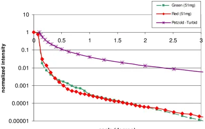
0.00001 0.0001 0.001 0.01 0.1 1 10

0 0.5 1 1.5 2 2.5 3

angle (degree) n o rm al iz ed in te n si ty Green (51mg) Red (51mg) Petzold -Turbid

(68)

Ideally VSF can be calculated using measuring instruments which can measure the attenuation and extinction separately and back calculate the scattering coefficient for every angle [10].

Mie theory simulations are satisfactorily be performed for the polystyrene spheres due to their spherical nature. The real part of the refractive index for is 1.56 while the complex part of the refractive index is considered negligible for simulations. The real and complex refractive index are directly associated with the scattering and absorption of the polystyrene spheres§. These simulations are carried out for the particles with diameter 500nm and 6 m. These results are compared with the experimental data for both operational wavelengths red and green. The normalized intensity is plotted for the near forward angles. 0.00001 0.0001 0.001 0.01 0.1 1 10

0 0.5 1 1.5

angle (degree) in te ns ity (n or m al iz ed )

Mie Theory for Red Experimental-Red (10mg)

Figure 4-16 Comparison of experimental measurements and Mie Theory prediction for 500nm latex spheres.

(69)

0.00001 0.0001 0.001 0.01 0.1 1 10

0 0.5 1 1.5 2 2.5 3

angle (degree) in te ns ity (n or m al iz ed )

Mie Theory for Green-6um

Experimental-Green (10.2mg)

Figure 4-17 Comparison of normalized experimental measurements and Mie theory predictions of scattering from for 6 m latex spheres.

The Mie simulation results and experimental data are normalized to emphasize the strong agreement in the shape of the two curves.

The beam spread patterns of light beams show an exponential decay for most water conditions. With increasing link length the beam attenuation will increase exponentially, i.e. decrease in the intensity of light. When compared to Gaussian distribution of the beam at the source, the expanded beam would have a much larger radius. The intensity distribution for can be given as follows [11]:

2

2_/

2r w oe I

(70)

Figure 4-18 Normalized Gaussian intensity distribution[11].

(71)

(72)

(73)

This gives us an insight into the beam dispersion, degradation in the spatial coherence and multipath time dispersion of the beam in the medium. From optical link standpoint, the multipath time spread is important, since it determines the maximum rate of communication [9]. Simulating each scenario using Monte Carlo method present fundamental difficulties, like defining the variables of the system accurately and sufficient computing power. Though Monte Carlo simulations have been used to support theories, but implementing it for all scenarios would be practically difficult. Hence, having an analytical model that would facilitate the evaluation of results would find great application in practical scenarios. Based on experimental results and in situ measurements we can extract useful information about the nature of scattering in a multiple scattering medium like ocean waters.

4.3 Beam Spread function

Beam spread function with time dispersion is an approach to quantify the contribution of scattering to the total attenuation of light [5]. This model relates the temporal spread of the light beam to the attenuation instead of the scattering coefficient itself. Each scattering event results in time delay, the average of multipath time delay is defined as the difference between the average transient time incurred from multiple scattering and the normal transient time in the absence of scattering. Since scattering can be treated as statically independent, the moments of multipath time dispersion can give a good idea of the scattering itself [4, 5].

The normalized radiative transfer equation can be presented as follows

(74)

where L(z, ,s, ) is radiance as a function of distance z, position , direction s, multipath time and Q is the energy.

Moments of the multipath time, displacement and directionality have been calculated with relation to scattering length (bz) [4]. The multipath time can be calculated using

) (t−z_c =

τ Eq. 4.6 c is the speed of light

z is the path length

The mean of the multipath time is found to be

) )( ( 4 1 2 c z bz θ

µτ = Eq. 4.7

Here b is the spectral scattering coefficient (b( )) of the medium.

2

θ is the mean-square scattering angle The variance of multipath time is found using

_σ2 =( )2

( )

1₁₂ _θ4 +

( )

1₂₄(bz)2 _θ2 2

τ z_c bz Eq. 4.8

Case 1 waters and parts of Case 2 waters observe forward scattering regime [1]. Our model assumes a characteristic scattering angle equal to 0.13 radians for calculations [5].

The analytical model suggests that the beam spread function with time dispersion is a product of a normalized temporal distribution function g(z, ) and a normalized spatial-angular distribution function h(z, ,s, ) [5].

(75)

where a is the spectral absorption coefficient (a( )) of the medium. The temporal distribution function g(z, ) is suggested to follow gamma distribution and is expressed as

− Γ = − 2 1 2 2 2

2 ₍ ₎ exp

) , ( 2 2 τ τ σ µ τ τ τ τ τ τ σ τ µ σ τ µ σ µ σ µ τ τ τ z

g Eq. 4.10

where and are the mean and standard deviation of the multipath time dispersion obtained using Equation 4.7 and Equation 4.8

The normalized spatial-angular distribution is configured for a time dependent case as below

= − − + z c z z s s c s z h . 3 . 3 exp ) ( 4 3 ) , , ,

( ₂ ₂ 2 2 2

τ

ρ

τ

π

τ

ρ

Eq. 4.11

If the average time t=

τ

c/z is replaced by 1₄(_bz _θ2 )_{Equation 4.10 becomes} time-independent. Equation 4.11 integrates over spatial and angular coordinates to yield Gaussian forms the enables the evaluation of the integrated beam spread function.

₂ 2 2

exp(

)

... ( , , , ) . .

(1

)

az

k z

s

d d ds

ac

µ στ τ

τ τ

ρ τ τ ρ

σ µ

−

=

+

Eq. 4.12

Equation 4.12 can be treated as the total beam attenuation in the multiple scattering medium. The equation is fundamentally an exponential decay function proportional to the absorption coefficient of the medium and the denominator quantifies the additional attenuation associated with multipath time delay caused by scattering.

(76)

source and receiver once the absorption and scattering coefficients are known. From an optical communication standpoint, it is important to know that this relation holds true for large field of view (FOV) receivers [18]

The beam attenuation given in Equation 4.12 and simulated by MathCAD** is shown in Figure 4-20. The simulation was done for a 1 W source operating at wavelength 532 nm. The beam attenuation versus depth is calculated for various chlorophyll concentrations. The spectral absorption and scattering coefficients are calculated using the one parameter model from Chapter 3.3 and 3.4.

Figure 4-20 Beam attenuation vs. Depth for different chlorophyll concentrations using source operating at 532nm.

(77)

4.4 Spectral Attenuation

With the introduction of the complete attenuation model, it is worthwhile taking a second look at the beam attenuation k( ) along the visible spectra. With the MathCAD model the wavelengths corresponding to minimum attenuation for various chlorophyll concentrations are found to shift to higher wavelengths and in shown Table 4-1

Table 4-1 Wavelengths corresponding to minimum attenuation for different chlorophyll-a concentrations

!"

" ! )

%

* ) ) + + )

(78)

Figure 4-21(a) Wavelengths corresponding to minimum attenuation for different chlorophyll concentrations using MathCAD model.

(79)

4.5 Beer’s law and beam spread function comparison

Traditionally the transmission losses between the source and receiver have been calculated using Beer’s law [11, 12].

_._exp (c( ).L)

Tx Rx P

P ₌ − λ _{Eq. 4.13}

Where c( ) is the spectral attenuation coefficient and L is the distance between source and receiver. The spectral attenuation coefficient c( ) is the sum of the absorption coefficient and scattering coefficient [1, 2].

) ( ) ( )

(λ a λ b λ

c = + Eq. 4.14

Equation 4.14 relates the attenuation directly proportional to the scattering coefficient. The beam spread function is not in agreement with this relation. A comparison is carried out between the beam spread function and Beer’s law. For a given scenario of a 1 W source operating at 532 nm and receiver sensitivity of -30dBm, the maximum possible link length was calculated for the two approaches. These calculations were performed in MathCAD for different chlorophyll concentration. The maximum link lengths offered by the Beers law and the beam spread function are plotted in Figure 4-22. The difference between them with respect to the beam spread function is also shown in the figure.

(80)

0 50 100 150 200 250 300 350

0 2 4 6 8 10 12 14

" ! ) % ,

-)# 0 10 20 30 40 50 60 70 80 90 100 . -)**

( #" - *+ )

( /#

. -)**

Figure 4-22 Percentage difference between Beer’s law and beam spread function for different concentrations of chlorophyll calculated using MathCAD.

4.6 Seawater Experiment

4.6.1 Introduction

(81)

Figure 4-23: Experimental setup for measuring attenuation in seawater

4.6.2 Experimental Setup

As the source of attenuation seawater was filled in an isolated water tank of dimensions 1m x 0.4m x 0.3m. Two runs of direct power measurements were carried out to exhibit attenuation by pure sea water and by chlorophyll added to sea water.

Two light sources: Green Laser (<5mW) and Red He-Ne Laser (1mW) were used for the experiment. The received radiant power is measured using a broadband power meter as depicted in the Figure 4-23 [13, 14].

4.6.3 Observations and Results

Underwater Free Space Optics

ABSTRACT

UNDERWATER FREE SPACE OPTICS

___________________________

__________________________

BIOGRAPHY

ACKNOWLEDGEMENTS

TABLE OF CONTENTS

LIST OF TABLES

LIST OF FIGURES

LIST OF ABBREVIATIONS

LIST OF SYMBOLS

( )

λ

( )

( )

( )

λ

( )

λ

( )

( )

( )

λ

( )

( )

( )

σ

τ

CHAPTER 1 INTRODUCTION

CHAPTER 2 OPTICAL PROPERTIES OF WATER

λ

λ

λ

λ

σ

λ

π

σ

CHAPTER 3 BIO-OPTICAL MODELS

λ

λ

λ

λ

λ

λ

λ

λ

λ

λ

λ

λ

λ

λ

σ

π

σ

σ

CHAPTER 4 PATHLOSS

β

θ

θ

θ

πρ

θ

θ

θ

0

0.5

1

1.5

2

2.5

3

( )

( )

τ

ρ

ρ

τ

_λ

_λ

_λ

_λ

_λ