Three Essays on Trend Analysis and Misspecification in Structural Econometric Models

(1)

ABSTRACT

DOORN, DAVID JOHN. Three Essays on Trend Analysis and Misspecification in Structural Econometric Models. (Under the direction of Alastair Hall)

The purpose of this research has been to look into several econometric issues of concern to researchers doing applied work in macroeconomics. The first essay looks at Bureau of Economic Analysis data on inventories and sales of finished goods often used in studies of inventory behavior. Applying recently developed methods, the series are rigorously tested to determine their stationarity properties. Results indicate that neither first differencing nor linearly detrending the data is appropriate. For most series a trend function with one or more breaks offers a better fit and also generates stationarity. The results are used to determine the impact on estimation in a simple production-smoothing model of inventory behavior. The impact of different trend specifications on univariate forecasting of inventories is also considered.

The second essay considers an alternative method of detrending time series data – the Hodrick-Prescott (HP) filter. Previous research has shown that HP filtering can have serious adverse consequences when used to analyze co-movements between data series at business cycle frequencies. Despite this, the filter has also been used to induce stationarity in a data series prior to estimation of structural econometric models. Little work has been done in analyzing the possible effects this may have on parameter estimates from such models. A simulation study is conducted to assess the impact of HP filtering on parameter estimation and a comparison is made to other detrending methods. It is shown that the HP filter induces bias in the parameter estimates and also increases the root mean squared error of the estimates from the simulations. In addition, there is some adverse impact on the size of certain test statistics.

(2)

THREE ESSAYS ON

TREND ANALYSIS AND MISSPECIFICATION

IN STRUCTURAL ECONOMETRIC MODELS

by

DAVID JOHN DOORN

A dissertation submitted to the graduate faculty of

North Carolina State University

in partial fulfillment of the

requirements for the Degree of

Doctor of Philosophy

ECONOMICS

Raleigh

2003

APPROVED BY:

_ _

Chair of Advisory Committee

(3)

Biography

(4)

List of Tables

1.1 Summary Statistics . . . 24

1.2 Adjustment Factors . . . 24

1.3 Prior Research . . . 25

1.4 ADF Test: Optimal Lags and Results . . . 25

1.5 Elliot et al. Critical Values . . . 26

1.6 Test Results . . . 26

1.7 Zivot and Andrews’ Critical Values . . . 26

1.8 Lumsdaine and Papell Critical Values . . . 27

1.9 Structural Breakpoints and Test Results for Single-Break Models . . . 27

1.10 Breakpoints and Test Results for Two Breaks in Trend . . . 28

1.11 Selected Models For Detrending . . . 28

1.12 Estimation Results From Deterministic Detrending Procedures . . . 29

1.13 Choice ofpfrom SIC . . . 29

2.1 Cost Parameters for Simulation Study . . . 66

2.2 Speciﬁcation of Sales Process and Cost Shock Parameters . . . 66

2.3 Implied Parameters of Inventory Process . . . 66

2.4 Implied Values of Regression Coeﬃcients . . . 66

(7)

3.1 Examples of Papers Performing Inference Based on Misspeciﬁed Models . . . 127

3.2 Calibrated Parameter Values By Industry . . . 128

3.3 Implied Population Values of Model Parameters . . . 129

3.4 Large Sample Probability Limits By Speciﬁcation & Weight Matrix . . . 130

3.5 Rejection Rates of J_T-test (%), Average Noise Ratios (NR¯ ), and Noise Ratio Model Selection by Speciﬁcation and Weight Matrix. . . 131

3.6 Limiting Distributions for Alternative GMM Estimators and the JT Test Statistic . . . . 132

3.7 Estimation Results for the Full Model . . . 133

3.8 Estimation Results for the Pure Model . . . 135

3.9 Estimation Results for the Stockout Avoidance Model . . . 136

3.10 t-statistic Rejection Rates: Pure Model . . . 138

3.11 t-statistic Rejection Rates: Stockout Avoidance Model . . . 139

(8)

List of Figures

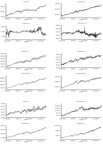
1.1 Time Series of BEA Inventory and Sales Data . . . 30

1.2 Time Series of BEA Inventory and Sales Data . . . 31

1.3 Sequential t-tests: Selected Models — Inventories . . . 32

1.4 Sequential t-tests: Selected Models — Sales . . . 33

1.5 Detrending Models and Residuals . . . 34

1.8 Forecasts . . . 37

1.9 Forecasts . . . 38

1.10 Forecasts . . . 39

2.1 Frequency Response of HP Cyclical Filter . . . 70

2.2 Spectral Density of Total Aggregate Inventories of Non-Durables . . . 71

2.3 HP and Linear Trends . . . 72

2.4 Residuals . . . 73

2.5 ACF . . . 74

2.6 Density ofβ₁ Estimates. . . 75

2.7 Density ofβ₂ Estimates. . . 76

(9)

Chapter 1

Trend Breaks in Finished Goods

Inventories and Sales of

Non-Durables

1.1 Introduction

Much research in recent years has focused on the role of inventories in explaining business cycles. While

inventory investment is generally a very small component of GDP, it has been noted in the literature

that most recessions tend to be periods of high inventory dis-investment, with changes in inventories

accounting for 87% of the fall in GDP, on average, for postwar recessions in the U.S. (see, for example,

Blinder and Maccini (1991) or Ramey and West (1997)). This indicates the importance of looking at

inventory behavior when considering the possible causes of business cycles as well as their persistence.

Unfortunately, most models of inventory behavior perform poorly with respect to the empirical facts

and there has not yet been a widely accepted solution to this problem.

(10)

inap-stationary for the asymptotic econometric theory to hold. The widely applied Generalized Method of

Moments (GMM) in particular requires stationarity of the variables contained in the moment condition

on which estimation is based. Prior research has tended to choose data transformations that are based

upon little or no formal testing prior to estimation, often choosing a linear or quadratic de-trending

procedure. This study takes advantage of recent advances in the unit root literature and applies a

num-ber of previously unavailable testing procedures to data on inventory and sales for six industries and

aggregate non-durables. This allows for a more informed determination of the stationarity properties of

the data prior to estimation, rather than just choosing a convenient transformation based upon a small

amount of evidence or common practice.

Initially, the commonly used Augmented Dickey-Fuller test for unit roots is applied to the data

and the results presented. Then a more powerful class of tests is applied in an attempt to get stronger

results. Lack of convincing evidence from these tests indicates the need for further testing, which initially

includes the presence of a single break in the trend function for the stationary alternative in the unit

root tests. These tests are then expanded to include the possibility of a second break in trend for these

series. Most of the series tested are found to contain either one or two breaks in trend and this result is

then applied in detrending the data. The resulting transformations do result in stationary series.

Given these results, a comparison is made to see if there is a signiﬁcant impact on estimation results

from a commonly used inventory model. The model is estimated using three diﬀerent detrending

pro-cedures to attain stationarity in the data. These include detrending based on the presence of a linear

trend, a quadratic trend, and a piecewise linear trend. Surprisingly, there is not a lot of diﬀerence in

results obtained from the three deterministic detrending methods. We also find that first-differencing

does give quite diﬀerent results, but these tend to be implausible given both the underlying theory and

the empirical facts.

In addition, the diﬀerent detrending procedures imply quite diﬀerent time paths for the series. A look

at the implications of these results for forecasting of inventories is also undertaken. Not surprisingly,

(11)

choosing a forecasting model and also illustrates the impact that the use of unit root tests may have on

this selection.

The paper will proceed as follows: Section 1 describes the data series used in the analysis and

includes an update of the adjustment suggested in West (1983) to put the inventory and sales series

on a comparable measurement basis. Section 2 describes the unit root tests applied to the series and

presents the results. Section 3 discusses the choice of detrending model for each series based on the tests

in Section 2. Section 4 describes a simple model of inventory behavior and compares estimates using

diﬀerent detrending procedures. Section 5 discusses the implications of the test results from section 2

for forecasting of inventories. Section 6 concludes with a summary of the results.

1.2 The Data

The data series used in this study is one that is commonly employed in the Inventory literature. This is

the Bureau of Economic Analysis (BEA) data on end-of-month ﬁnished goods inventories and sales. The

BEA series are gleaned from the Census Bureau’s Manufacturer’s Shipments, Inventories, and Orders

(M3) survey and are used in estimation of the National Income and Product Accounts (NIPA) for the

calculation of GDP. The data are adjusted to constant chained 1992 dollars from the book values reported

by ﬁrms in the raw M3 data. The procedures used are described in the Survey of Current Business,

published monthly by the BEA. The data employed here are consistent with the procedures described

in the August 1998 issue of the Survey. The monthly series are also seasonally adjusted, using the X-12

method, and cover the periods January 1959 through May 1998. This yields 473 observations.

To be consistent with prior research using the linear-quadratic model of inventory behavior, we

concentrate on the six two-digit SIC industries commonly considered as being production to stock.

These include Food, Tobacco, Apparel, Chemicals, Petroleum, and Rubber. Also considered is the series

for overall non-durables manufacturing, which adds Textiles, Paper, Printing, and Leather to the above.

(12)

cost. To make the data consistent across series it is necessary to adjust either inventories or sales by the

ratio of market price to unit cost, evaluated in the base year. West suggests an approximation to this

ratio that can be constructed from IRS data. This approximation takes the form: (business receipts)

÷(cost of sales and operations + rent + repairs + depreciation + taxes). Table 1.2 gives the resulting

adjustment factor using a 1992 base for each of the six two-digit industries and for total non-durables.

In incorporating the adjustment the sales series were divided by the adjustment factor. The adjusted

sales series should then be used in estimation. For much of the single series descriptive analysis that

follows, however, this adjustment is inconsequential and so the unadjusted series are used.

A precursory look at the time series plots of the data suggests the possibility of a deterministic

trend for all of the series, except perhaps for Tobacco sales and Tobacco inventories. It is of course

also possible that the data follow a unit root with drift process. Most of the literature using this data

tends to assume some kind of polynomial time trend and so de-trend the data using standard methods

to attain stationarity. Very few of the studies actually discuss any unit root testing of the data to

determine its stationarity properties, and those that do tend to report somewhat ambiguous results.

Nearly all of the studies end up using deterministically detrended data, with some also repeating their

work with diﬀerenced data, e.g. Eichenbaum (1989); Durlauf and Maccini (1995). Table 1.3 lists some

of the prior research on inventories and what, if any, testing was reported on the data used, as well

as the transformations applied prior to its use. Because there seems to be no compelling evidence in

the literature, this study rigourously investigates the stationarity properties of the data using recently

developed tests from the unit root literature.

1.3 Unit Root Testing

In analyzing the data several diﬀerent tests for the presence of unit roots were applied. These include the

standard Augmented Dickey-Fuller test, the point optimal tests of Elliot et al. (1996), and extensions of

the ADF test that include the possibility of breaks in the trend function.1 All of these tests are based

(13)

on some form of equation 1.1 withd(t) indicating a deterministic function of time. The speciﬁcation of

d(t) is the primary diﬀerence between the tests applied.

yt= ˆαyt−1+d(t) + k

j=1

ˆ

cj∆yt−j+ ˆet (1.1)

Thekautoregressive ∆yt₋j terms are included to allow for the possibility of auto-correlation in the

disturbances, which may cause problems in the limiting distributions of the test statistics. It has been

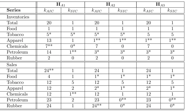
noted in the literature on unit-roots that the number of extra regressors, k, included in Equation 1.1 can impact the power and the size of unit root tests. Hall (1994) shows that using pretest data-based

model selection procedures to choosekcan greatly increase the power of the ADF test. We employ two of these procedures here to choose the number of extra regressors to include for each data series in each

test, the Akaike information criteria (AIC) and the Schwartz information criteria (SIC).2

Both the AIC and the SIC are designed to choose thekthat minimizes a criterion function over all possible lag lengths considered, with the diﬀerence being in the speciﬁed criterion function. The criterion

to be minimized takes the form:

T ln(T−1SSRk) +CR, (1.2)

whereSSRk is the sum of squared residuals from 1.3 and CR is 2(k+ 2) for AIC and (k+ 2)ln(T) for

SIC. Under certain conditions it can be shown that the probability that ˆkSIC is the truekis one in the

limit, while there is a positive probability that ˆkAIC is greater than the true k.3 This means that it is

possible for AIC to overﬁt the model. In ﬁnite samples the nature of the penalty functions, CR, requires

that ˆkSIC ≤ ˆkAIC once T attains a certain size. Of the following testing procedures, the three ADF

tests make use of both AIC and SIC, while the rest only apply SIC to determine the number of lags to

include. Unless otherwise noted, the maximum lag-length allowed was 25 for all series.

2_{We also used the Hannan and Quinn procedure reported in Hall (1994), but found the results to be virtually identical}

to either the SIC or AIC for every series and so chose not to report it.

(14)

1.3.1 Augmented Dickey-Fuller Tests

The ﬁrst tests undertaken were standard augmented Dickey-Fuller (ADF) tests. Three versions of these

tests were applied to the data, with the ﬁrst being a test of the unit root with drift hypothesis against

a single-mean stationarity alternative and the second being the same null against stationarity about a

linear trend. In addition, some of the authors in Table 1.3 speciﬁed a quadratic trend function when

detrending the data, so a third test of the unit root null against quadratic-trend stationarity was also

applied. The trend function for these tests is of the form

d(t) =µ+βt+γt2, (1.3)

withβ andγrestricted to zero for tests against the single-mean stationarity alternative andγrestricted to zero for the linear-trend speciﬁcation.

The null hypothesis based on equation 1.1 is H0 : α= 1 and a t-statistic is constructed from the regression to test this assertion. This t-statistic is then compared to the tables formulated in Dickey and

Fuller (1979, 1981) for the single-mean and linear-trend alternatives andH0is rejected for small values of t. For the quadratic-trend alternative p-values were calculated using the response-surface methods outlined in MacKinnon (1994). The number ofk extra regressors chosen and the results of these tests are given in Table 1.4.

1.3.2 Point-Optimal Tests

In addition to the ADF tests, two tests proposed by Elliot et al. (1996) were used, both of which

were shown to have better size and power properties than the above tests and several others that have

been suggested in the literature. The ﬁrst of these is a modiﬁed version of the ADF test used above,

which Elliot et al. term the DF-GLS test, since it uses a type of generalized least-squares procedure

in generating the test statistic. The second test is a simple scaled likelihood-ratio constructed by the

(15)

Equation 1.1. ¯αis chosen to be the alternative for which maximal power of the tests are approximately .5, which Elliot et al. show will cause the statistic to lie close to the Gaussian power envelope over a large

range. They suggest using ¯α= 1 + ¯c

T, where ¯c =−7 for tests against a constant mean and ¯c=−13.5

for tests against a linear trend speciﬁcation. The tests used here are only those against the alternative

of linear trend stationarity.

The DF-GLS test uses a procedure to demean and detrend the series of interest, yt, to obtainyDt ,

which is then used in place of yt in equation 1.1. In this cased(t) becomes zero, so the test using the

transformed series is against zero-mean stationarity.

The detrending procedure involves a number of steps. To begin with, the data series is transformed

to obtainyα_¯= (y1, y2−αy¯ 1, ..., yT −αy¯ T−1). Then deﬁne the trend speciﬁcation in aT×qmatrix,Z,

wherezt= (1) for the constant mean case andzt= (1, t) for the linear trend case. TransformZto obtain Zα_¯= (z₁, z₂−αz¯ ₁, ..., zT−αz¯ T₋₁). We then run a regression ofyα_¯ onZα_¯ to obtain an estimate for the

coeﬃcient vector on the trend speciﬁcation, ˆβ. This estimate is then used to constructyD

t =yt−βˆzt,

the detrended and demeaned series used in the test.

The PT-statistic is constructed as

PT =

[S( ¯α)−αS¯ (1)] ˆ

ω2 (1.4)

whereS(x) is the sum of squared residuals from the regression ofyxonZx, withyx= (y1, y2−xy1, ..., yT− xyT₋₁) and Zx = (z₁, z₂−xz₁, ..., zT −xzT₋₁) and the ztare as above. The denominator, ˆω2, is an

estimator of ω2 = ∞_k₌_−∞γ(k), where γ(k) = Evtvt₋k are the autocovariances of the error. The

estimator used here is the autoregressive estimator described in Elliot et al.. This is

ˆ

ωAR2 =

ˆ

ση2

(1−p_i₌₁ˆai)2

(1.5)

with ˆση2 and ˆai being the OLS estimates from the regression

∆yt=a0yt−1+ p

i₌₁

(16)

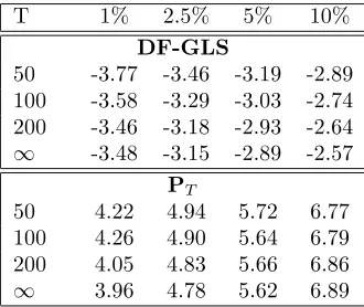
These test statistics do not follow any of the usual tables of critical values, so Elliot et al. conduct

Monte Carlo simulations to generate appropriate critical values. The critical values for each of these

tests against the alternative of linear trend stationarity are reproduced in Table 1.5. The results for the

inventory and sales series are given in Table 1.6, using the asymptotic critical values from Elliot et al..

1.3.3 Tests Allowing For Breaks In The Trend Function

One conclusion from the literature on unit roots has been that a mis-speciﬁcation of the trend function,

d(t), can result in the appearance of a unit root when in fact one does not exist. Because of this we also conduct tests that allow for the possibility of shocks to the series at certain dates. These shocks,

if they exist, may cause a break, or a shift, in the trend of an otherwise trend-stationary series. One

way of testing this in the context of unit roots in general was derived by Perron (1989), in which several

macroeconomic data series were tested. Perron performed a visual inspection of the series and concluded

that there were two possible trend breaks, the Great Depression and the 1973 oil crisis. The series were

then tested for unit roots using a speciﬁcation that allowed for the possibility of a break in trend at one

of these points.

For many of the inventory and sales series in the current study a visual inspection of the data is an

unsatisfactory means of determining the possible existence of a structural breakpoint, and so other ways

of making this determination are desirable. Zivot and Andrews (1992) and Banerjee et al. (1992) also

take issue with Perron’s method of determining breakpoint and devise procedures to choose the most

likely date for a break in trend for each series. Their procedures assume that the structural change at

these points is endogenous, and so data dependent, rather than exogenous. This leads to tests in which

the null hypothesis of a unit root with drift, which implies there is no structural change, is set against

the alternative of stationarity about a deterministic trend, with possible changes in the trend function

at some point in time. This null can be formulated as

(17)

While these authors only consider the possibility of a single break in trend, Ben-David et al. (1996)

and Lumsdaine and Papell (1997) derive a general extension to include two breaks in the trend function.

The general form for the trend function in all of these models becomes:

d(t) = ˆµ+ ˆβt+ ˆθDU1t(ˆλ) + ˆγDT1t(ˆλ) + ˆωDU2t(ˆλ) + ˆψDT2t(ˆλ) (1.7)

where λi = TBi/T, with TBi being the date at which the break occurs for i = 1,2; DU it(λ) = 1 if t > T λ, 0 otherwise;DT it(λ) =t−T λift > T λ, 0 otherwise.

We conduct tests based on equation 1.1 with six variants of this trend function, three that allow for

the presence of a single break, and three that allow for two breaks. Model A imposes the restriction

ˆ

γ= ˆω= ˆψ= 0, and so only allows for the possibility of a one-time shift in the overall level of the series, or its mean. Model B includesd(t) with ˆθ= ˆω= ˆψ= 0, which only allows for a one-time change in the slope of the deterministic trend. Model C includes d(t) with ˆω = ˆψ= 0, which allows for a change in both mean and level at a single date. These three models are identical to those considered in Zivot and

Andrews (1992). Banerjee et al. also consider models A and B,4 but in a more complex notation, and

attain similar results to those of Zivot and Andrews.

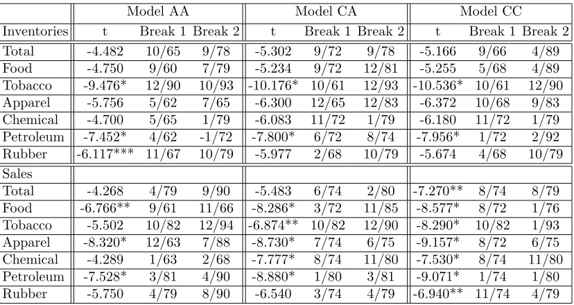
In addition we consider the two-break models of Ben-David et al. (1996) and Lumsdaine and Papell

(1997). Model AA includesd(t) with ˆγ= ˆψ= 0, and so allows for two shifts in the mean of the series.

Model CA imposes only ˆψ = 0, and so allows for one break in which the mean shifts and another in

which both the mean and the slope of the series change. Finally, Model CC makes no restrictions ond(t) in equation 1.7, which allows for both a shift in mean and a change in slope at two possible breakpoints.

The testing strategy is to construct at-statistic testingα= 1 at each possible trend breakpoint, or combination of breakpoints, and then choosing those breakpoints that produce the minimum t-statistic

as being the ones of interest.5 This results in choosing breakpoints which give the most weight to the

alternative of trend stationarity. In practice this requires estimation of each model at each possible

breakpoint, or set of breakpoints, using ordinary least squares. This process includes determining the

(18)

this, the SIC procedure described above was employed for each possibleλ, with the maximum possible lag length of 25 for the single-break models and, due to the extra computational burden, 12 for the

two-break versions.6

As in the ADF testing above, the t-statistics here will not have the same distribution as the standard

t-statistic, due to the inclusion of lagged ﬁrst-diﬀerences of the regressor. Nor are they comparable to the

ADF tables. For the single-break tests, Zivot and Andrews have compiled the appropriate tables for each

of the three models mentioned above using Monte Carlo methods, both for the asymptotic distribution

and for the ﬁnite-sample distribution of the test statistic. Due to the relatively large sample size employed

here, we consider the asymptotic results to be the more appropriate tables to use for comparison. The

ﬁndings of Banerjee et al. with regard to sample size indicate there is little variation in the critical values

for sample sizes greater than 250, again lending support to the use of the asymptotic critical values. The

critical values generated by Zivot and Andrews are reproduced in Table 1.7.7 Similarly, the appropriate

critical values for the two-break tests have been calculated by Lumsdaine and Papell (1997) and are

given in Table 1.8.

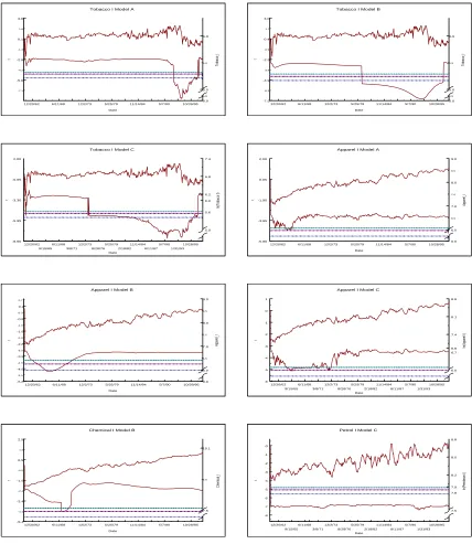
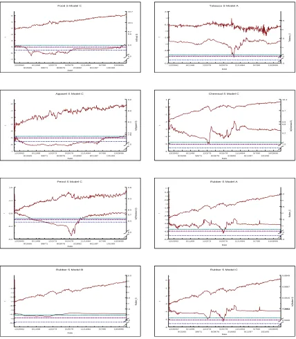
Table 1.9 gives the minimum t-statistic for each series and for each model in the single breakpoint

case, also indicating the date at which the corresponding structural break is determined to have taken

place. Similar results for the two-break tests are reported in Table 1.10. The signiﬁcance of the test

for each series and each model is also given. For the single-break tests it will also be useful to look at

selected results graphically. Figures 1.3 and 1.4 plot a few of the time series along with the t-statistic

generated using each date as a breakpoint. To save space only selected plots are given. The 1%, 5%,

and 10% asymptotic critical values are indicated as well in each diagram.

1.4 Choice of Detrending Models

We now have plenty of test results with which to determine the fate of our data. By looking at each

series separately we can combine the results from the standard unit root tests with those found using

6_{It should be noted that Zivot and Andrews use a diﬀerent procedure to determine} _k_{. However, we chose the SIC}

(19)

other methods from the literature, along with visual inspection of the time series, to decide upon the

most likely trend speciﬁcation. In doing this we are ignoring the possible implications of the results

for any type of modeling that might be done using these data. These results are solely the product of

univariate testing procedures to determine the time series properties of each series and to aid in choosing

the best transformations to achieve stationarity.

To begin with, three of the fourteen series would appear be linear trend stationary. Petroleum

inventories, Food sales, and Apparel sales all provided strong evidence against a unit root in the initial

ADF, as well as in the more powerful DF-GLS and PT testing procedures. Tests allowing for a break

in trend produced evidence against unit roots at nearly every possible breakpoint for these three series.

This can be seen in the plot of Model C for these series.8 Additional ADF tests for stationarity on either

side of the most likely breakpoints also seems to lend support to this ﬁnding. This points to a simple

linear detrending procedure as the best transformation for these series.

For Tobacco inventories, while there was evidence of linear trend stationarity in the initial tests, the

evidence was somewhat weaker using the DF-GLS and the PT tests. A visual inspection of the series

also gives a clear indication of a break in trend at one or more points. Including the possibility of a single

breakpoint resulted in Model A giving the most plausible result, with a break in trend in December of

1993. Allowing for a second break in trend at some point also seemed to give plausible results, with

December 1993 again showing up as a possible breakpoint, along with various earlier possibilities. In

deciding between the use of a single break model or a two break model in detrending the data it would

seem most appropriate to choose the model which requires the least amount of changes to the original

series and still attain stationarity. Even though the two break results are somewhat visually appealing,

this criterion would lead us to choose the single break model for this series. Tests on the resulting

subsamples indicate linear-trend stationarity on the ﬁrst period, but cannot reject a unit root in the

later subsample. This may be due to the short length of this subsample.

Apparel inventories, Chemical inventories, and Petroleum sales all presented little or no evidence

(20)

did result in rejections of the null for all three series, with Model B proving the most plausible approach

for the two inventory series and Model C for Petroleum sales. Tests allowing for two breaks in the trend

function found no evidence against unit roots for Apparel inventories or Chemical inventories, but did for

the Petroleum sales series. This leads to the choice of single break models for the two inventory series,

with a break in trend in September 1966 for Apparel and March 1969 for Chemicals. While for the

Apparel series this choice is well supported by tests of subsamples on either side of the break, the same

is not true for the Chemical series. It remains the only choice, however, given the other test results. For

Petroleum sales we do have signiﬁcant two-break tests for each model, but again we have the case where

a less intrusive procedure will give the desired result, and so Model C with a single break at February

of 1980 is chosen for detrending this series. This choice also is well supported by tests on either side of

the break.

There was no evidence against the presence of a unit root for any of the initial tests or for the

single break tests on the Rubber inventory series. Only Model AA of the two break tests provided any

signiﬁcant evidence for detrending this series. This leads us to choose this model with breakpoints at

November 1967 and October 1979 for transforming the data. Tests of the subsamples on either side of

and in between these breakpoints found signiﬁcant evidence against a unit root only for the subsample

after the last breakpoint, and then only at a 10% signiﬁcance level.

Total sales also presented evidence against a unit root only for one of the double trend break tests.

This was model CC, which gave break dates of August 1974 and August 1979. Tests on the subsamples

surrounding these dates provided evidence against unit roots for all three at the 5% level.

Tobacco sales and Chemical sales each found little support for a linear trend speciﬁcation using the

ﬁrst three tests. The single break models also found only weak evidence against the null, with tests on

either side of the breakpoints adding little support. Model CC of the two-break tests found strong support

at the 1% level for rejection of a unit root for both of these series, however. The indicated breakpoints

are October 1982 and January 1993 for the Tobacco series and August 1974 and November 1980 for

(21)

Tobacco, both the subsample up to the ﬁrst break and that after the second found support for linear

trend stationarity at the 10% level. The middle subsample could not reject the presence of a unit root.

For Chemicals, only the subsample after the second breakpoint was signiﬁcant in its rejection of a unit

root, and this at the 5% level. Despite this the double break speciﬁcation would seem to be the most

appropriate to use in transforming the series.

While there seems to be some support for specifying a linear trend with no breaks for the Rubber

sales series, the evidence isn’t as strong as it was for the three series above for which we decided upon

this speciﬁcation. In tests for a single break in trend for this series there was strong evidence against

a unit root for both Models C and A, with both giving the same break date of April 1979. Tests on

either side of this date found only weak evidence of trend stationarity for the subsample prior to this

date. Testing for two breaks in trend produced the same break date as above and also the earlier date

of November 1974. All tests on the subsamples about the two breaks were signiﬁcant in their rejections

of unit roots at the 5% level. This lends strong support for using model CC for detrending.

This leaves two series for which we have yet to make a determination. Both the Total Inventories

and Food inventories series found no evidence for rejecting the unit root in any of the above testing

situations, aside from the PT test on Total Inventories. It is likely that the reason for this is that we

haven’t found a trend speciﬁcation which adequately ﬁts the data, since this may lead to the appearance

of a unit root process. It is possible that allowing for more breaks in the trend may solve this problem.

Unfortunately the computational burden of extending the two-break test above to include three or more

possible breaks is prohibitive. In addition, new critical values would need to be calculated. Applying

the single-break tests to subsamples on either side of the breakpoints chosen initially also did not result

in any signiﬁcant rejections of the null. Arguably, the best choice to make in this case would be a model

that is most likely to be closest to the true trend speciﬁcation, so we should include as many breaks

as possible. Also, since tests on either side of the breakpoints given by the single break models were

insigniﬁcant, it would seem that a two-break speciﬁcation is more appropriate. For the Food series, a

(22)

at the 5% level against a unit root for the fairly long sample in between. The other two subsamples

indicated no rejection of a unit root process. For Total inventories we had two models give the same

break dates of September 1966 and April 1989. Tests of the resulting subsamples again found rejection

of the null at the 5% level for the middle sample while no evidence for rejection in the others. This

would seem to be as good as we can get for these two series.

The models chosen for transformation of the individual series to attain stationarity are summarized

in Table 1.11. Graphs of the detrending models and the resulting stationary residuals are presented in

Figures 1.5 through 1.7.9 ADF tests on the detrended series found all of them to reject the presence of

a unit root at a 5% conﬁdence level against a zero mean stationarity alternative.

While prior researchers have generally chosen to apply a linear detrending procedure to this data, they

seemed to base this decision on little evidence. The results shown here indicate that, while detrending

may be the correct thing to do, simply removing a linear trend from all of the series is inappropriate.

Even though inventory and sales behavior may be similar across industries, there is no reason to expect

that shocks to these series will happen in all of the industries at the same time or that their trends will

be aﬀected in the same way.10 It is likely that, while things that aﬀect the economy as a whole may

aﬀect these industries in similar ways, idiosyncratic shocks may take place within each industry that

cause the paths taken in their inventory and sales behavior to be divergent. This indicates that each

industry should have its own trend speciﬁcation.

One of the main results of the unit root literature has been in pointing out the importance of correct

speciﬁcation of trend functions. Lack of this results in the appearance of unit roots and the problems in

inference that go along with them. Here we have attempted to discover trend speciﬁcations that at least

are likely to result in stationary series after their use in detrending. There is fairly strong evidence that

the trend speciﬁcations chosen here do this. One potential problem with these results is that for many

of the industries we found breaks in trend for the inventory series that do not seem to be related in any

way to breaks in the sales series. The papers in which the trend break methods were introduced applied

9_{These graphs were generated using the}_EasyReg _{program of Herman Bierens.}

(23)

them only to single data series, with no mention of the implications when those series are then used in

combination to estimate some structural model of the economy. The implications of this for models of

inventory behavior are not entirely clear.

1.5 Impact on Parameter Estimates from a Linear-Quadratic

Model of Inventory Behavior

1.5.1 The L-Q Model

One model of inventory behavior that has been prevalent in the literature is the linear-quadratic (L-Q)

model, so called because it assumes that demand is linear and both production costs and inventory costs

are quadratic, indicating rising marginal costs. Generally, the model is expressed in such a manner that it

includes several possible motivations for and characteristics of inventories. These may include production

smoothing, stock-out avoidance, costs of adjusting production, autocorrelated cost shocks, exogenous or

endogenous sales, and demand shocks.11 While the theoretical constructs of the model seem plausible,

empirical work has by and large rejected the L-Q model in its diﬀerent forms. In particular, the many

studies using this model have come up with a wide range of parameter estimates that are often at odds

with each other and diﬃcult to defend given the empirical facts. The most contentious result has been

that the estimated speed of adjustment between actual inventories and desired levels tends to be much

too slow given industry production capacity.

A simple form of the linear-quadratic inventory model is based on a representative ﬁrm choosing the

level of inventories that will minimize the present value of costs, including both costs of production and

of holding inventories. This can be represented by the following equations:

min

It+j ∞

j₌₀

βjEt[CQ(Qt+j) +CI(It+j, St+j)] (1.8)

(24)

CQ(Qt+j) = ( δ

2)Q

2

t₊j (1.10)

CI(It+j, St+j) = ( φ

2)(It+j−ωSt+j)

2 _(1.11)

where It is end of period inventories,St is exogenous real sales,Qt is real production,β is a constant

discount rate, andEt(•) =Et(• |Ωt) is the mathematical expectations operator, with Ωtthe information

available at time t. The three structural parameters of the model include δ, the marginal cost of

production, φ, the cost associated with inventories being other than the desired level, and ω, the cost associated with back-orders or stock outs.

All of the parameters are assumed to be non-negative constants. This assumption indicates that

production costs are convex. With δ > 0, a production-smoothing motive is implied, meaning ﬁrms

will meet demand shocks partially out of inventories to avoid additional production costs. Forω = 0,

φ reflects holding costs of inventories, with costs rising with stock. This also will result in production smoothing, given that all the other parameters are greater than zero. Forω >0, there is a buffer stock motive — firms will want to hold inventories to fill unexpected orders rather than risk back ordering.

The ﬁrm must then weigh the cost of holding extra inventory against that of stock outs.

The solution to the above results in the following Euler equation:

Et[δQt+φ(It−ωSt)−βδQt₊₁] = 0 (1.12)

This implies that the ﬁrm will choose an inventory level such that the cost of making and storing an

additional unit this period provides no cost beneﬁt over waiting to produce the unit in the next period.

Substituting in for production yields

Et[δ(St+It−It−1) +φ(It−ωSt)−βδ(St+1+It+1−It)] = 0 (1.13)

which can then be solved forIt+1:

(25)

This can be rearranged and expressed as the second-order diﬀerence equation

Et[(1−λL)(1−(λβ)−1L)It+1] =Et[ α

βSt−St+1] (1.15)

with α= 1−φω_δ , L representing the lag operator, and λand (λβ)−1 being the roots of the equation: 1−ΦL+β−1L2 , where Φ = (1+_ββ)+_βδφ. With the structural parameters all non-negative, 0< λ <1 andα≤1.

Solving the equation for optimalItyields

It=λIt₋₁−St+ (1−αλ)Et[ ∞

j=0

(λβ)jSt₊j] (1.16)

This relation implies several characteristics for ﬁrm’s inventory decisions. Inventories are positively

related to expected future sales, while being negatively related to current sales. This indicates that ﬁrms

meet current sales out of inventories rather than increase production. It can be shown that the above

model accommodates the stock adjustment model sometimes seen in the literature (see Eichenbaum

(1989) for details), a basic version of which is: It= (1−λ)[It∗−It−1]. HereIt∗ is some desired level of

inventories, usually dependent onEtSt, and 1−λthe per period speed of adjustment towards that level.

In order to estimate the model, Equation 3.9 is usually expressed as a moment condition and then the

Generalized Method of Moments (GMM) is applied to attain parameter estimates. While the structural

parameters are not all identiﬁed, it is possible to come up with estimates for λ and α. Most of the literature restrictsβ to be .995 in estimation. The moment condition becomes

EtF(Ht+1;θ) =Et[(1−λL)(1−(λβ)−1L)It+1+St+1− α

βSt] = 0 (1.17)

where Ht+1 = [It+1 It It−1 St+1 St] and θ = [α λ β]. Expanding the right hand side yields the

following estimable version of the equation:

EtF(Ht₊₁;θ) =Et[It₊₁−(λ+ (λβ)−1)It+β−1It₋₁+St₊₁− α

βSt] = 0 (1.18)

Unfortunately, the various studies using this model have come up with a wide range of parameter

(26)

output being more variable than sales in most industries. Of course the inclusion of a buﬀer stock

motive may help to explain this. Also the model implies a negative relationship between current sales

and inventory investment, which again is at odds with the empirical facts. This also may be partially

explained through the positive relationship between inventories and expected future sales. If current

sales are unexpectedly high, it is likely that ﬁrms will adjust forecasts of future sales to reﬂect this, thus

explaining the pro-cyclicality of inventories. Despite these problems the linear-quadratic model has been

used in a great number of studies to date, mostly in attempts to ﬁnd reasonable speeds of adjustment

to desired inventory levels, which can be represented as approximately 1−λ.

1.5.2 Impact on Parameter Estimates

The main point of unit root testing is to attain stationarity in the data series used in estimation of

economic models. This is necessary for the statistical theory underlying most estimation procedures

to hold. While the eﬀects of diﬀerencing when there is a deterministic trend or, in the opposite case,

applying a deterministic detrending procedure to a stochastically trending process are well documented,

it may be interesting to look at the effects of different deterministic detrending specifications on the

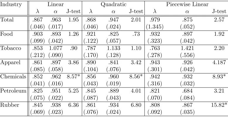
parameter estimates from our inventory model. The following is a comparison of the GMM estimation

results from the L-Q inventory model when three diﬀerent detrending procedures are used on the data.12

All results are from iterated GMM estimation with instrument set including a constant and two lags

each of inventories and sales.13 The detrending procedures include a linear trend speciﬁcation for both

sales and inventories, a quadratic trend speciﬁcation for both series, and ﬁnally the piecewise linear

detrending implied by the above results. Parameter estimates and the J-test of model speciﬁcation are

shown in Table 1.12 .

Given the imprecision of the parameter estimates, particularly forλ, it is diﬃcult to gauge whether

12_{The model was also estimated with diﬀerenced data. However the resulting estimates for}_α_{were either greater than}

one or negative, which is counter to the assumptions of the model. Therefore we do not report these estimates.

13_{In estimating the model, equation 1.18 was multiplied by}₋_βλ_{to obtain a diﬀerent normalization. The result gives}

(27)

the diﬀerent detrending procedures have a great impact. It is notable, however, that use of piecewise

linear detrending results in decidedly larger standard errors in most instances. In addition, there seems

to be little impact on the J-statistics testing model speciﬁcation. Only in the case of the Rubber industry

does the change in detrending procedure aﬀect the results of the speciﬁcation test.

1.5.3 Other Implications

Despite the fact that there seems to be little eﬀect on the outcome for this model, the above trend

speciﬁcations do imply permanent changes in the growth paths of the sales and inventory series at the

break dates. While previous research has indicated persistence in the inventory-sales relationship,14 if

a shift in trend for the sales series is not accompanied by a corresponding shift in inventories, then the

relationship between these two variables is permanently changed. Likewise for shifts in inventories that

do not induce shifts in sales. In the context of the L-Q model, this implies that the structural parameters

may change at these breakpoints. This can be seen in reference to the moment condition in Equation

1.18.

In order for this moment condition to remain true after a permanent shift in the growth path of just

one of the series, there must be a change in one or more of the parameters at that point. This means

that marginal costs will have changed at these points. One possible way to test for this would be to

estimate the model using subsets of the data deﬁned by the breakpoints. If the resulting estimates diﬀer

signiﬁcantly, then this conclusion is supported. Other tests of structural change could also be applied

to the model to determine if the parameters do in fact change over the series’ histories. However, the

current study is intended to determine if diﬀerent detrending methods will aﬀect the parameter estimates

and such structural change tests are left for future consideration.

14_{Ramey and West (1997), using quarterly and annual data for the U.S., report impulse response curves indicating that}

(28)

1.6 Forecasting

Another area where choice of model speciﬁcation in a univariate sense can have an impact is in forecasting

models. In this case stationarity is not the goal. Instead we are looking to develop a model that performs

well in producing accurate forecasts. It has recently been shown in Diebold and Kilian (2000) that using

the results from unit-root tests to decide between use of a random walk with drift or a linearly trending

AR(1) process in forecasting a data series can lead to lower prediction mean squared errors (PMSE).

Given this, it is also likely that different choices of trend specification will result in markedly different

forecasting results.

Using the inventory series from above, we can look at the impact of three diﬀerent model speciﬁcations

on out-of-sample forecasts. These models are a random walk with drift, a linearly trending AR(p) process, and an AR(p) with piecewise linear trend using the breakdates speciﬁed in Table 1.11.15 The choice ofp

is that chosen by the SIC pre-test model selection procedure outlined above. These choices are listed in

Table 1.13. The trend speciﬁcations given in the table are the result of unit root tests using this selection

procedure, so it seems prudent to include those autoregressive terms in our forecasting models.16 We are

interested in looking at the diﬀerences in time paths implied by the out-of-sample forecasts from these

diﬀerent models. Determining the correct trend speciﬁcation ought to greatly improve forecasts from

any model. It would be expected that basing out-of-sample forecasts on a model with breaks should

give quite a diﬀerent result than the other models, since the breaks represent a discreet change in the

deterministic path of the series which isn’t present in the linear model. The question then becomes how

far out in the forecast horizon do we get before this diﬀerence becomes signiﬁcant. Figures 1.8 through

1.10 show the out-of-sample forecasts for each model applied to each series.17 The results are in levels

(millions of dollars) so as to get a better idea of the magnitude of the diﬀerences between them. The

15_{Using a quadratic trend in a forecasting model does not seem to be a reasonable speciﬁcation. Since the coeﬃcient}

on the quadratic trend term is generally negative, the longer the forecast horizon, the more dominant this term is likely to be as the forecasts converge to the series’ long run trend. We did look at this for the inventory series and for three of the series the quadratic trend model resulted in declining inventories into the future. For the three series in which this specification does not result in a declining forecast, the quadratic trend coefficient is either insignificant or very nearly so. For Total inventories a quadratic trend model did not converge to give parameter estimates.

16_{Campbell and Perron (1991) and Cochrane (1991) do simulations which include such pre-determined lagged variables}

(29)

forecast horizon goes out to 120 periods, or ten years.

Notably, for Rubber inventories the forecasts of all three models are nearly indistinguishable for the

whole forecast horizon. The maximum diﬀerence, after 120 periods, is $52million between the linear

forecast and the piecewise linear. Recall, however, that a unit root was not rejected for this series for

any of the tests with the exception of Model AA, which rejected at the 10% level. It is interesting to see

that the wrong choice of forecasting model in this case would not have a great impact on the results,

even at long horizons. Unfortunately, this is unlikely to be true for most other forecasting applications,

as we shall see.

Also interesting are the forecasts for the Tobacco industry. The random walk model forecasts declining

inventories right from the start. Both the linear and piecewise linear models give a diﬀerent picture,

with forecasts being very close to each other for several periods before diverging. It is diﬃcult to see in

the ﬁgure, but these two forecasts reach a maximum diﬀerence at 68 periods. From there the piecewise

forecasts level out somewhat and the diﬀerence between the two shrinks as the forecasts from the linear

model approach those from the piecewise. Apparently they will cross at some point in the distant horizon.

Despite this, it is still obviously important to choose the right model from the start, as the maximum

diﬀerence in levels between the linear and piecewise models is over $100 million and the random walk

model gives an even greater diﬀerence in levels. In this case, the piecewise linear model was chosen in

the unit root testing and therefore should give the most reliable forecasts.

For Food inventories we found that a unit root was not rejected in any of the above testing procedures.

This suggests that the random walk model should be the one chosen for forecasting. Surprisingly, the

piecewise linear model gives forecasts that are fairly close to those from the random walk at short

horizons. The diﬀerence doesn’t reach $100 million for thirty-two periods, nearly three years. With

inventories in the twenty billion dollar range, this may be acceptable. The forecasts from the linear

model are lower and quickly diverge from those of the other two.

For Apparel inventories our testing indicates that the piecewise linear model is the best choice. Again

(30)

However, at the end of the 120 periods we have a diﬀerence of more than $800 million between these

models. Again there is a quick divergence in the linear model’s forecasts, resulting in a diﬀerence of

more than $1400 million from the piecewise model at the end of the forecast horizon. Again we see that

the choice of model clearly will have a signiﬁcant impact at long horizons.

For Total inventories we had no rejections of a unit root from any of our testing other than the PT

test. This indicates a random walk model for forecasting. In this case, the linear model remains fairly

close to the random walk for several periods before reaching a diﬀerence of $100 million at the 12th

period. The maximum diﬀerence between these two is $910 million at the end of the forecast horizon,

which may not be too bad considering the inventory levels are in the $100 billion range. However, the

piecewise linear model results in a diﬀerence of nearly $5 billion from the random walk forecast at the

end of the horizon.

Finally, for both Chemicals and Petroleum we have a quick divergence between the two models

applied in each case. For Petroleum, a linear trend model was strongly indicated by the tests. Using

a random walk model quickly leads to a diﬀerence of more than $10 million within two periods and

a diﬀerence of more than $760 million by the end of the horizon. Clearly the choice of model has an

impact in this case regardless of forecast horizon. For Chemicals our tests indicate a single break model

as the best ﬁt. Applying a random walk results in extreme diﬀerences in forecasts almost immediately,

$48 million in the ﬁrst period and rising to more than $.5 billion in nine months. At the end of the

forecast horizon we see a diﬀerence of more than $5.6 billion.

While the ﬁgures indicate point forecasts that can diﬀer greatly as we move further out in the forecast

horizon, by billions of dollars in some cases, only for three of the industries do the point forecasts for

the random walk with drift or the linear trend speciﬁcation follow paths which takes them outside of the

forecast interval for the piecewise linear model. These are Food, Apparel, and Chemicals. For Food it

takes 74 periods for the linear model to give a forecast result that lies outside of this interval. For Apparel

it takes 75 periods for this to happen. For Chemicals, the linearly trending model did not converge, but

(31)

These results give an indication that choosing forecasting models on the basis of unit root tests can

result in a signiﬁcant diﬀerence from just choosing a linear trend or random walk model. By including

the possibility of breaks in trend for these series we get another choice in our modelling. Apparently

this also can have a signiﬁcant impact on forecasting results. Interestingly, at short horizons there was

not a great diﬀerence in forecasts from some of the models in some of the industries. As Diebold and

Kilian (2000) suggest, it would be interesting to expand their study to see whether these types of trend

speciﬁcations being included in unit root tests actually result in better forecasts when choosing models

on that basis.

1.7 Summary

This study has conducted a rigourous analysis of the time series properties of a widely used set of

inventory data. Applying recent advances in the unit root testing literature we ﬁnd that when including

the possibility of one or more breaks in trend for each series, we can reject the presence of a unit root

in most cases. With these results in hand we choose models for detrending that remove piecewise linear

or linear deterministic trends from each of the series to attain stationarity. The resulting transformed

data is then used to test if there is any impact on the estimation results from a popular model of

inventory behavior when using different trend specifications for detrending. We find that the type

of trend speciﬁcation does not greatly aﬀect parameter estimates from the model or tests of model

specification based on GMM. However, standard errors do seem to be significantly affected by the type

of detrending procedure used.

In addition, there has been much interest in determining whether unit root tests are useful in the

selection of forecasting models. Again using the results from the unit root tests above we look at the

impact that diﬀerent models have on forecasts out to 120 periods. We ﬁnd that in many cases the models

other than the one selected in testing result in quite diﬀerent forecasts, especially at long horizons. While

(32)

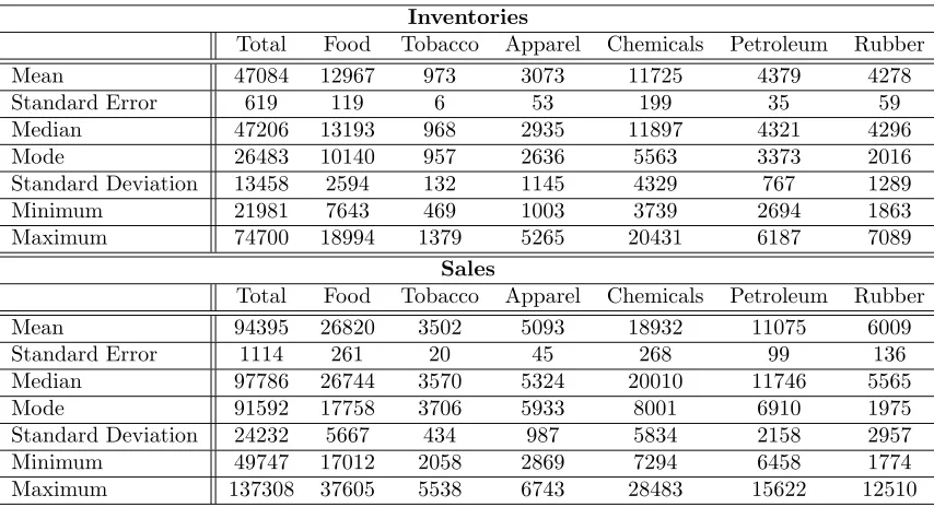
Table 1.1: Summary Statistics

Inventories

Total Food Tobacco Apparel Chemicals Petroleum Rubber

Mean 47084 12967 973 3073 11725 4379 4278

Standard Error 619 119 6 53 199 35 59

Median 47206 13193 968 2935 11897 4321 4296

Mode 26483 10140 957 2636 5563 3373 2016

Standard Deviation 13458 2594 132 1145 4329 767 1289

Minimum 21981 7643 469 1003 3739 2694 1863

Maximum 74700 18994 1379 5265 20431 6187 7089

Sales

Total Food Tobacco Apparel Chemicals Petroleum Rubber

Mean 94395 26820 3502 5093 18932 11075 6009

Standard Error 1114 261 20 45 268 99 136

Median 97786 26744 3570 5324 20010 11746 5565

Mode 91592 17758 3706 5933 8001 6910 1975

Standard Deviation 24232 5667 434 987 5834 2158 2957

Minimum 49747 17012 2058 2869 7294 6458 1774

Maximum 137308 37605 5538 6743 28483 15622 12510

Data is in in millions of chained 1992 dollars

Table 1.2: Adjustment Factors

Series Adjustment Factor

Food 1.3354

Tobacco 1.7044

Apparel 1.3056

Chemicals 1.4998

Petroleum 1.1465

Rubber 1.3185

(33)

Table 1.3: Prior Research

Paper Data Years Transformation Reported

Unit Root Tests

Blinder (1986) BEA 1959:2 - 1981:12 detrended none

Blinder and Maccini (1991) BEA 1959:1 - 1986:10 detrended none

Durlauf and Maccini (1995) BEA 1959:1 - 1990:6 detrended yes, but

un-speciﬁed

Eichenbaum (1989) BEA 1959:1 - 1984:12 separately

de-trended and

diﬀerenced

none

Fuhrer et al. (1995) BEA 1967:1 - 1991:8 none none

McCarthy and Zakrajsek (1998) BEA

Trade Goods

1959:1 - 1997:8 diﬀerenced panel data

version of

ADF

Miron and Zeldes (1988) BEA &

M3

1967:5 - 1982:12 detrended only none

Ramey (1991) BEA &

M3

1959:1 - 1979:12 detrended none

Ramey and West (1997) BEA &

Citibase

1959:1 - 1996:4 none none

Schuh (1996) M3LRD 1985 - 1993 detrended none

West (1990) Citibase 1947:1 - 1986:4 diﬀerenced Said-Dickey

Table 1.4: ADF Test: Optimal Lags and Results

HA1 HA2 HA3

Series kAIC kSIC kAIC kSIC kAIC kSIC

Inventories

Total 20 1 20 1 20 1

Food 1 1 1 1 1 1

Tobacco 5* 5* 5* 5* 5 5

Apparel 13 1 1** 1** 1** 1**

Chemicals 7** 0* 7 0 7 0

Petroleum 14 1** 3* 3* 3* 3*

Rubber 2 0 2 0 2 0

Sales

Total 24** 1 24 1 24 1

Food 4 1 1* 1* 1* 1*

Tobacco 12 5 12 5 12 5

Apparel 12 2 2* 1* 2* 1*

Chemicals 12 1** 12 1 12 1

Petroleum 23 2 23 0** 23 0**

Rubber 24 1 24** 0* 24 0*

(34)

Table 1.5: Elliot et al. Critical Values

T 1% 2.5% 5% 10%

DF-GLS

50 -3.77 -3.46 -3.19 -2.89

100 -3.58 -3.29 -3.03 -2.74

200 -3.46 -3.18 -2.93 -2.64

∞ -3.48 -3.15 -2.89 -2.57

PT

50 4.22 4.94 5.72 6.77

100 4.26 4.90 5.64 6.79

200 4.05 4.83 5.66 6.86

∞ 3.96 4.78 5.62 6.89

Table 1.6: Test Results

DF-GLS PT

Inventories

Total -0.798 1.148*

Food -2.058 9.788

Tobacco -2.462 6.033***

Apparel -1.409 18.114

Chemicals -0.542 95.417

Petroleum -3.509* 1.927*

Rubber -1.30 26.206

Sales

Total -0.939 36.349

Food -3.501* 3.815*

Tobacco -1.979 12.542

Apparel -2.679*** 4.435**

Chemicals -0.799 61.212

Petroleum -2.716*** 6.303***

Rubber -2.453 5.501*

* indicates significance at the 1% level ** indicates significance at the 5% level *** indicates significance at the 10% level

Table 1.7: Zivot and Andrews’ Critical Values

Model 1% 2.5% 5% 10% 50% 90% 95% 97.5% 99%

A -5.34 -5.02 -4.80 -4.58 -3.75 -2.99 -2.77 -2.56 -2.32

(35)

Table 1.8: Lumsdaine and Papell Critical Values

Model 1% 2.5% 5% 10%

AA -6.94 -6.53 -6.24 -5.96

CA -7.24 -7.02 -6.65 -6.33

CC -7.34 -7.02 -6.82 -6.49

Table 1.9: Structural Breakpoints and Test Results for Single-Break Models

Model A Model B Model C

Inventories t Date t Date t Date

Total -3.564 Sept. 1978 -3.175 Jan. 1967 -3.515 Nov. 1971

Food -4.217 July 1979 -3.558 May 1988 -4.391 Dec. 1981

Tobacco -8.205* Dec. 1993 -7.281* July 1992 -8.267* Dec. 1990

Apparel -4.770*** Oct. 1964 -5.022* Sept. 1966 -5.135** Nov. 1965

Chemical -3.926 May 1965 -4.449* March 1969 -4.561 July 1972

Petroleum -7.087* April 1962 -7.045* May 1963 -7.415* Feb. 1992

Rubber -4.236 Oct. 1979 -2.881 Dec. 1968 -4.374 Oct. 1979

Sales

Total -3.734 April 1979 -3.964 July 1972 -4.740 April 1979

Food -6.516* Nov. 1966 -6.122* Oct. 1972 -6.489* Nov. 1966

Tobacco -4.954** Oct. 1982 -2.925 May 1993 -4.654 Oct. 1982

Apparel -6.068* July 1988 -6.162* Dec. 1967 -6.253* Dec. 1978

Chemical -3.975 Feb. 1968 -4.222*** Feb. 1972 -5.000*** Aug. 1974

Petroleum -5.115** Feb. 1981 -6.234* Nov. 1976 -8.346* Feb. 1980

Rubber -5.110** April 1979 -4.298*** April 1972 -5.327* April 1979

(36)

Table 1.10: Breakpoints and Test Results for Two Breaks in Trend

Model AA Model CA Model CC

Inventories t Break 1 Break 2 t Break 1 Break 2 t Break 1 Break 2

Total -4.482 10/65 9/78 -5.302 9/72 9/78 -5.166 9/66 4/89

Food -4.750 9/60 7/79 -5.234 9/72 12/81 -5.255 5/68 4/89

Tobacco -9.476* 12/90 10/93 -10.176* 10/61 12/93 -10.536* 10/61 12/90

Apparel -5.756 5/62 7/65 -6.300 12/65 12/83 -6.372 10/68 9/83

Chemical -4.700 5/65 1/79 -6.083 11/72 1/79 -6.180 11/72 1/79

Petroleum -7.452* 4/62 -1/72 -7.800* 6/72 8/74 -7.956* 1/72 2/92

Rubber -6.117*** 11/67 10/79 -5.977 2/68 10/79 -5.674 4/68 10/79

Sales

Total -4.268 4/79 9/90 -5.483 6/74 2/80 -7.270** 8/74 8/79

Food -6.766** 9/61 11/66 -8.286* 3/72 11/85 -8.577* 8/72 1/76

Tobacco -5.502 10/82 12/94 -6.874** 10/82 12/90 -8.290* 10/82 1/93

Apparel -8.320* 12/63 7/88 -8.730* 7/74 6/75 -9.157* 8/72 6/75

Chemical -4.289 1/63 2/68 -7.777* 8/74 11/80 -7.530* 8/74 11/80

Petroleum -7.528* 3/81 4/90 -8.880* 1/80 3/81 -9.071* 1/74 1/80

Rubber -5.750 4/79 8/90 -6.540 3/74 4/79 -6.940** 11/74 4/79

* indicates significance at the 1% level ** indicates significance at the 5% level *** indicates significance at the 10% level

Table 1.11: Selected Models For Detrending

Inventories Model Break Dates

Total CC September 1966 and April 1989

Food CC May 1968 and April 1989

Tobacco A December 1993

Apparel B September 1966

Chemical B March 1969

Petroleum Linear None

Rubber AA November 1967 and October 1979

Sales

Total CC August 1974 and August 1979

Food Linear None

Tobacco CC October 1982 and January 1993

Apparel Linear None

Chemical CC August 1974 and November 1980

Petroleum C February 1980

(37)

Table 1.12: Estimation Results From Deterministic Detrending Procedures

Industry Linear Quadratic Piecewise Linear

λ α J-test λ α J-test λ α J-test

Total .867 .963 1.95 .868 .947 2.01 .979 .875 2.57

(.046) (.017) (.046) (.024) (1.345) (.052)

Food .903 .893 1.26 .921 .825 .73 .932 .897 1.92

(.099) (.042) (.122) (.057) (.323) (.042)

Tobacco .853 1.077 .90 .787 1.133 1.10 .763 1.421 2.20

(.212) (.090) (.170) (.128) (.278) (.556)

Apparel .861 .897 3.86 .890 .841 3.42 .943 .926 4.187

(.085) (.058) (.104) (.076) (.301) (.042)

Chemicals .852 .962 8.57* .856 .960 8.56* .942 .932 8.93*

(.041) (.016) (.043) (.019) (.316) (.032)

Petroleum .825 .951 5.25 .845 .889 4.01 .821 .684 3.21

(.075) (.022) (.087) (.043) (.070) (.084)

Rubber .845 .938 6.36 .861 .934 6.80 .808 .867 15.82*

(.069) (.023) (.076) (.024) (.092) (.035)

* indicates the model specification is rejected at the 95% level

Table 1.13: Choice ofpfrom SIC

Model

Industry Linear Piecewise Linear

Total 2 1

Food 2 2

Tobacco 6 1

Apparel 2 2

Chemicals 1 2

Petroleum 4 na

(38)

3/25/60 3/8/71 2/18/82 1/31/93 Date 7000 12000 17000 Food_I

3/25/60 3/8/71 2/18/82 1/31/93 Date

20000 30000 40000

Food_S

3/25/60 3/8/71 2/18/82 1/31/93 Date

600 1000 1400

Tobacco_I

3/25/60 3/8/71 2/18/82 1/31/93 Date 2000 3000 4000 5000 6000 Tobacco_S

3/25/60 3/8/71 2/18/82 1/31/93 Date 1000 2000 3000 4000 5000 6000 Apparel_I

3/25/60 3/8/71 2/18/82 1/31/93 Date 2000 3000 4000 5000 6000 7000 Apparel_S

3/25/60 3/8/71 2/18/82 1/31/93 Date 5000 10000 15000 20000 Chemical_I

3/25/60 3/8/71 2/18/82 1/31/93 Date

10000 20000 30000

Chemical_S

3/25/60 3/8/71 2/18/82 1/31/93 Date 2000 3000 4000 5000 6000 7000 Petrol_I

3/25/60 3/8/71 2/18/82 1/31/93 Date 7000 9000 11000 13000 15000 Petroleum_S

3/25/60 3/8/71 2/18/82 1/31/93 Date 2000 4000 6000 8000 Rubber_I

3/25/60 3/8/71 2/18/82 1/31/93 Date

4000 9000 14000

Rubber_S

(39)

3/25/60 3/8/71 2/18/82 1/31/93 Date

20000 30000 40000 50000 60000 70000 80000

Total_I

3/25/60 3/8/71 2/18/82 1/31/93 Date

40000 50000 60000 70000 80000 90000 100000 110000 120000 130000 140000

Total_S

Three Essays on Trend Analysis and Misspecification in Structural Econometric Models

THREE ESSAYS ON

TREND ANALYSIS AND MISSPECIFICATION

IN STRUCTURAL ECONOMETRIC MODELS

by

DAVID JOHN DOORN

A dissertation submitted to the graduate faculty of

North Carolina State University

in partial fulfillment of the

requirements for the Degree of

Doctor of Philosophy

ECONOMICS

Raleigh

2003

APPROVED BY:

___________________________ ___________________________

Chair of Advisory Committee

Biography

Contents

List of Tables

List of Figures

Chapter 1

Trend Breaks in Finished Goods

Inventories and Sales of

Non-Durables

1.1

Introduction

1.2

The Data

1.3

Unit Root Testing

1.3.1

Augmented Dickey-Fuller Tests

1.3.2

Point-Optimal Tests

1.3.3

Tests Allowing For Breaks In The Trend Function

1.4

Choice of Detrending Models

1.5

Impact on Parameter Estimates from a Linear-Quadratic

Model of Inventory Behavior

1.5.1

The L-Q Model

1.5.2

Impact on Parameter Estimates

1.5.3

Other Implications

1.6

Forecasting

1.7

Summary

_ _