What's All the Fuzz About? Effects of FIA Spatial Precision on the Performance of Species Distribution Models.

(1)

ABSTRACT

DIRENZO, JOSEPH ANTHONY. What’s All the Fuzz About? Effects of FIA Spatial Precision on the Performance of Species Distribution Models. (Under the direction of Ross Mentemeyer).

The Forest Inventory and Analysis (FIA) program of the United States Forest Service

(USFS) provides geographically extensive measurements of forest structure and composition

across the continental United State of America. FIA data are often used in species

distribution models (SDMs) to relate species occurrence or abundance at known locations

with environmental and/or spatial characteristics. However, in compliance with the Food

Security Act of 1985 (H.R. 2100) as amended by the Department of the Interior and the

Related Agencies Appropriations Act (H.R. 3423) in 2000, the United States Forest Service

is required to protect the location of FIA plots and identity of the land owners who’s land

may house an FIA plot. Therefore, spatial coordinates provided in the publically available

FIA data are “fuzzed”. In this study, our objective was to determine whether fuzzed

coordinates affected SDM results and assess the extent to which the spatial grain of

environmental predictors matters (100 m to 1000 m, in 100 m increments). We modeled the

occurrence and abundance of six species with small to broad environmental niches with

environmental covariates extracted to either the true or fuzzed plot coordinates. For all

species, the environmental covariates at each sample site did not significantly differ between

the use of fuzzed and true data coordinates within grain size. There was little variability in

prediction accuracy between fuzzed and true coordinate models of species occurrence or

abundance across grain sizes for each species. The grain of environmental covariate data

influenced precision but not accuracy, where many of the environmental covariates shared

(2)

coordinates in SDMs of large tree species and that future researchers can use finer scale

(3)

(4)

What’s All the Fuzz About? Effects of FIA Spatial Precision on the Performance of Species Distribution Models.

by

Joseph Anthony DiRenzo

A thesis submitted to the Graduate Faculty of North Carolina State University

in partial fulfillment of the requirements for the degree of

Master of Science

Natural Resources

Raleigh, North Carolina

2016

APPROVED BY:

________________________________ _________________________________

Ross Meentemeyer James McCarter

Committee Chair

(5)

BIOGRAPHY

Joe was born in Connecticut to a Colombian mother, Gloria Elena, and an Italian

father, Federico Joseph, in 1988. A love of all things living inspired him to graduate from

Southern Connecticut State University with a B.S. in Biology in 2011. Joe has volunteered

saving sea turtles in Costa Rica, studied lupin in Iceland, and hugged oak trees in California.

In the summer of 2015, while pursuing his graduate degree, he married Emily, the love of his

life. Together they enjoy pondering the meaning of life, gazing at the countless stars in the

(6)

ACKNOWLEDGMENTS

I’d like to thank Ross Meentemeyer, my advisor, for taking a chance on. It was a

pleasure working with him in the CAGIS lab at UNC at Charlotte and the Center for

Geospatial Analytics at NCSU. I’d like to thank Jim McCarter and Bob Abt, for being on my

committee and for the all the help and support. I’d like to thank my good friend Whalen and

my sister Grace for all the help and support. Finally, I’d like to thank my mother Gloria, my

brother Johnpaolo, and my loving wife Emily, for all the support you all have offered and

given me over the past few years.

(7)

LIST OF TABLES

Table 1. Description of environmental variables used in species distribution models ... 14 Table 2. Results of the paired t-tests between estimated parameter values of environmental covariates from true and fuzzed coordinates for each species. Each mini-table represents the species, the rows contain grain sizes, and the columns list the environmental variables. The cells within the tables list the corresponding p-values. Asterisks (*) indicate a statistically significant difference (* p<0.1, ** p<0.05, *** p<0.01). The abbreviations in the table follow

as: PPT, mean total yearly precipitation (1981-2010); PSI, potential solar irradiance

(calculated for the 183rd day (July 2nd) of 2014); TMIN, monthly mean of minimum daily

temperature (1981-2010); TWI, topographic wetness index. PIPO, Pinus ponderosa; PSME, Pseudotsuga menziesii; QUAG, Quercus Agrifolia; QUDO, Quercus douglasii; SESE,

Sequoia semprevirens; UMCA, Umbellularia californica. ... 15

Table 3. Results of the paired t-tests between 100 m true coordinate models (assumed to be the most accurate) and all other grain sizes and coordinate types for each species. Black text indicates comparisons between the 100 m true coordinate model output compared to other grain sizes using true coordinates. Red text indicates comparisons between the 100 m true coordinate model output compared to the output of models using fuzzed coordinates. Each mini-table represents the species, the rows contain grain sizes, and the columns list the environmental variables. The cells within the tables list the corresponding p-values. Asterisks (*) indicate a statistically significant difference (* p<0.1, ** p<0.05, *** p<0.01).

Abbreviations in the table follow as: PPT, mean total yearly precipitation (1981-2010); PSI,

potential solar irradiance (calculated for the 183rd day (July 2nd) of 2014); TMIN, monthly

mean of minimum daily temperature (1981-2010); TWI, topographic wetness index. PIPO, Pinus ponderosa; PSME, Pseudotsuga menziesii; QUAG, Quercus agrifolia; QUDO,

Quercus douglasii; SESE, Sequoia sempervirens; UMCA, Umbellularia californica. ... 16

Table 4. Accuracy metric means and standard deviation for models using true and fuzz coordinate data models at each resolution for each species. Black indicates TRUE model. Red indicates FUZZ model. Bold indicates greater accuracy. Asterisks (*) indicate a

statistically significant difference (* p<0.1, ** p<0.05, *** p<0.01) in means of the accuracy metric between TRUE and FUZZ models for the species at the resolution. Abbreviations follow as: Occurrence accuracy metrics: AUC, area under curve; COMMISSION, false positive rate (type I error) ; OMISSION, false negative rate (type II error); TSS, true skill statistic. Abundance accuracy metrics: COR, Pearson correlation coefficient; RMSE, root

mean square error, units in square meters (m2). PIPO, Pinus ponderosa; PSME,

Pseudotsuga menziesii; QUAG, Quercus Agrifolia; QUDO, Quercus douglasii; SESE,

(9)

Table 5. Accuracy metric means for true and fuzz coordinate models at each resolution for each species. Black indicates TRUE model. Red indicates FUZZ model. Bold indicates greater accuracy. Asterisks (*) indicate a statistically significant difference (* p<0.1, ** p<0.05, *** p<0.01) in means of the accuracy metric between the 100 m TRUE model and the corresponding TRUE or FUZZ model for the species at the resolution. Please refer to Table 3 for standard errors associated with accuracy metrics.Abbreviations follow as:

Occurrence accuracy metrics: AUC, area under curve; COMMISSION, false positive rate (type I error); OMISSION, false negative rate (type II error); TSS, true skill statistic. Abundance accuracy metrics: COR, Pearson correlation coefficient; RMSE, root mean

square error, units in square meters (m2). PIPO, Pinus ponderosa; PSME, Pseudotsuga

menziesii; QUAG, Quercus Agrifolia; QUDO, Quercus douglasii; SESE, Sequoia

(10)

LIST OF FIGURES

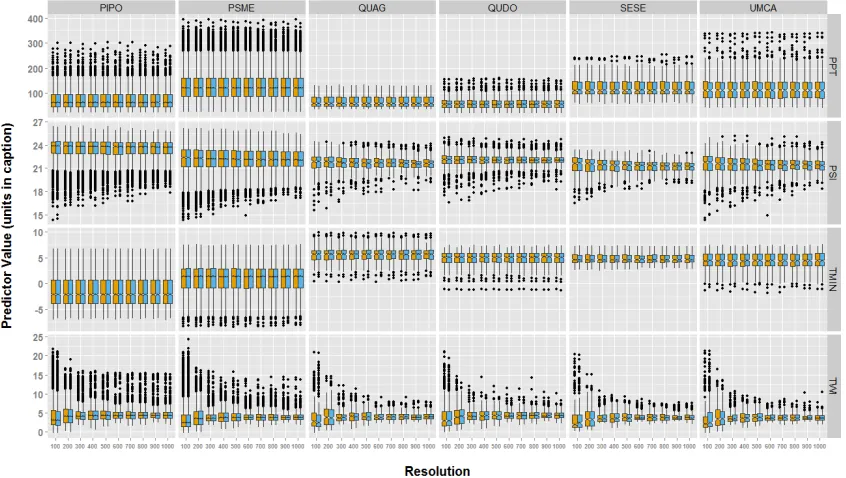
Figure 1. Estimated parameter values for each environmental variable (along the rows) for each species (along the columns) presence data used with true and fuzz coordinate. Yellow represents model run with fuzz coordinated. Blue represents models run with true

coordinates. Boxplots represent the interquartile range of estimated parameters around the line, which indicates the median parameter estimate. Points represent outlier values. The abbreviations in the figure follow as: PPT, mean total yearly precipitation (1981-2010), units

in mm; PSI, potential solar irradiance (calculated for the 183rd day (July 2nd) of 2014), units

in watt hours per square meter (WH/m2₎_{; TMIN, monthly mean of minimum daily temperature}

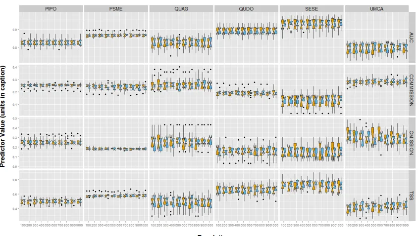
(1981-2010), units in °C; TWI, topographic wetness index, unitless. PIPO, Pinus ponderosa; PSME, Pseudotsuga menziesii; QUAG, Quercus agrifolia; QUDO, Quercus douglasii; SESE, Sequoia sempervirens; UMCA, Umbellularia californica. ... 11 Figure 2. Accuracy metrics for occurrence models with 10 fold cross validation. Species are along the columns, and accuracy metrics are along the rows. Yellow represents fuzzed

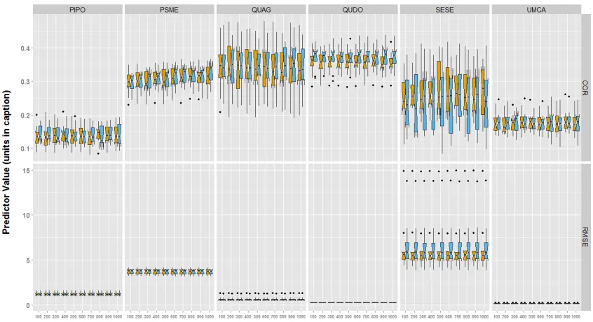
coordinates and blue represents true coordinates. Boxplots represent the interquartile range of estimated parameters around the line, which is the median value. Points represent outlier values. Abbreviations in the figure are as follows: AUC, area under curve; COMMISSION, false positive rate (type I error); OMISSION, false negative rate (type II error); TSS, true skill statistic. PIPO, Pinus ponderosa; PSME, Pseudotsuga menziesii; QUAG, Quercus agrifolia; QUDO, Quercus douglasii; SESE, Sequoia sempervirens; UMCA, Umbellularia californica. ... 12 Figure 3. Accuracy metrics for abundance models with 10 fold cross validation. Species are along the columns, and accuracy metrics are along the rows. Yellow represents models run with fuzzed coordinates and blue represents models run with true coordinates. Boxplots represent the interquartile range of estimated parameters around the line, which is the median value. Points represent outlier values. Abbreviations in the figure follow as: COR, Pearson

correlation coefficient; RMSE, root mean square error, units in square meters (m2). PIPO,

Pinus ponderosa; PSME, Pseudotsuga menziesii; QUAG, Quercus agrifolia; QUDO,

(11)

INTRODUCTION

The Forest Inventory and Analysis (FIA) program of the United States Forest Service

(USFS) is a national treasure. The program provides geographically extensive measurements of forest structure and composition across the continental United States. Forests are divided into 6000-acre hexagonal areas (Brand 2004) with long-term survey plots established at random locations within each area (Reams et al. 2005). Plots are typically re-measured at five-year intervals to detect the emergence of forest health problems (e.g. invasive pests and pathogens) and monitor demographic changes in growth, mortality, and recruitment of new individuals. The broad geographic extent of FIA data make it especially applicable for species distribution models.

Species distribution models (SDMs) relate species occurrence or abundance at known locations with the environmental and/or spatial characteristics of those locations (Elith & Leathwick 2009). They are used for aquatic or terrestrial plants or animals. SDMs have a broad spectrum of implications, including predicting species occurrence (Iverson & Prasad 1998) and species abundance (Fei & Steiner 2007, Harris 1999, Iverson & Prasad 1998) at unmeasured locations, the potential spread of an exotic species into a new spatial domain (Morin 2003), and potential shifts in species distributions under projected climate change scenarios (Iverson & Prasad 2002, Woodall et al. 2009, Gibson 2013, Serra-Diaz et al. 2016). To effectively model species distributions, it is important to consider what environmental factors constrain the species. Environmental variables may include precipitation,

temperature, elevation, light, distance to water, distance to forest edge, intensity of urbanization or agriculture, and many more, including variations of these. Spatial scale, including extent (the spatial domain of the study) and grain (the grid-cell size of the explanatory or predictor data) is integral to developing SDMs, and should be chosen based on the goals of the study and the nature of the data. Ideally, the grain of the explanatory data should align with the spatial accuracy and precision of the observed species data (Dungan et al. 2002, Tobalske 2002), however, this may not always possible.

In compliance with the Food Security Act of 1985 (H.R. 2100) as amended by the Department of the Interior and the Related Agencies Appropriations Act (H.R. 3423) in 2000, the USFS is required to protect the location of FIA plots and identity of the land

owners who’s land may house an FIA plot (www.fia.fs.fed.us). If precise plot coordinates are available, and overlaid on a surface containing parcel data and landowner information, it is possible to identify landowners to plots. Therefore, the precise coordinates of subplots are reported as existing up to 805m (½ mile) away from the true location of the plot in order to protect landowner privacy. In addition, attribute data from up to 20% of privately owned subplots are also substituted with attributes from similar subplots. These processes of moving coordinates and substituting attributes are termed “fuzzing” and “swapping”, respectively (www.fia.fs.fed.us). Fuzzing and swapping only occurs within county or supercounty (an aggregation of two or more adjacent counties in the same state) limits in order to maintain reliability of regional studies.

(12)

environmental data of at least 800m resolution (or coarser) would not likely express the situational differences existing between true and fuzzed locations Some analyses, however, may require the use of finer scale environmental data to be used in order to answer certain questions. Franklin et al. (2013) examined the differences of predicting climate refugia using fine and coarse grain predictors, and suggested that some climate refugia captured at finer scales may be missed using coarser scale data. In the same respect, studies such as that of Serra-Diaz et al. (2015), examining range shifts under climate change also require finer scale

environmental data in order to adequately address the issues at hand. While FIA data is

commonly used in SDM applications, it remains unclear if, how, and to what extent the use of fuzzed coordinates and correspondingly large resolution environmental data might affect analyses.

Several studies have examined the effects of fuzzed coordinates. Coulston et al. (2004) examined the influence of fuzzed plot locations on the accuracy of ordinary kriging and residual kriging estimates of forest biomass and found no statistically significant difference (α = 0.05) between the accuracy of models developed with the true FIA plot locations and models developed with fuzzed plot locations. The study did note, however, that accuracy was related to the spatial autocorrelation of the data. In a later study, Coulston et al. (2006) systematically examined the effects of fuzzed coordinates of simulated data with varying degrees of spatial autocorrelation on ordinary kriging and linear regression across different resolutions (30m, 250m, 500m, 1000m, 2000m). Their study showed that fuzzed plot locations did not significantly influence the accuracy of kriging estimates, but in some situations linear regression model accuracy was significantly influenced (decrease in R2

) as grain size of predictors and SAC decreased. These results suggest that unless the independent variable has high spatial autocorrelation, only coarse spatial resolution data should be used to develop linear regression models (Coulston et al. 2006).

McRoberts et al. (2005) conducted a design-based study for circular areas of increasing radii centered at either precise or fuzzed coordinates, and then compared the two. Their results suggest the effects of using fuzzed coordinates are negligible at any radii greater than approximately 32km. Most recently, Gibson (2013) found no statistically significant

differences in accuracy between using precise or fuzzed coordinates with predictor variables at1km resolution.

The general objective of this study is to determine the best resolution to model FIA data for use in species distribution modeling when predicting either occurrence or abundance of a tree species. We systematically address key issues to evaluate:

1) Do predictor variables extracted from fuzzed coordinates significantly differ from those extracted from precise coordinates and does the spatial grain of the variables matter?

2) Do fuzzed data differently affect the accuracy of species occurrence and abundance models and do accuracies vary with spatial grain?

(13)

We hypothesize that:

a) On average, as the grain size of the environmental data used decreases, predictor values will differ more between those extracted at TRUE coordinates vs. those extracted at FUZZ coordinates.

b) On average, occurrence models built with TRUE coordinates will increase in

accuracy as grain size of environmental data decreases; models built with FUZZ data will exhibit little to no change in accuracy as grain size of environmental data

decreases.

c) On average, abundance models built with TRUE coordinates will increase in accuracy as grain size of environmental data decreases; models built with FUZZ data will exhibit little to no change in accuracy as grain size of environmental data decreases. d) On average, models predicting occurrence or abundance for a specialist species will

be more sensitive to grain size and coordinate fuzzing than models predicting occurrence or abundance for generalist species.

METHODS

STUDY AREA

This study focuses on the states of California and Oregon. California and Oregon comprise a combined area of 262 075 sq. mi. and house most of the California Floristic Province (CFP) which is home to a great number of endemic species. This area, with its Mediterranean climate, is a hotspot for plant biodiversity (Myers & Mittermeier, 2000) and its land use changes (Thorne et al. 2009) and fire regimes (Dolanc et al., 2014) make it an excellent area

of interest to study changes in species occurrence and abundance. The topographically

heterogeneous nature of the study area also lends itself well to examining the effects of grain size on environmental variables.

SPECIES

Three conifer tree species (Pinus ponderosa,Pseudotsuga menziesii, and Sequoia

semprevirens) and three broad-leaved tree speces (Quercus Agrifolia, Quercus douglasii, and

Umbellularia californica) were chosen, representing specialist and generalist strategies

across a broad geographical region. Of the three conifers, P. ponderosa and P. menziesii are generalist species, occurring throughout much of the study area with their true ranges extending well beyond the borders of California and Oregon. S. semprevirens is a specialist species, occurring along the coast from Monterrey County in California to southern Oregon. Of the three broad leaf species, Q. douglasii is deciduous, and Q. Agrifolia and U. californica

(14)

OBSERVATIONAL DATA

The FIA database was queried for plot, species, true coordinates, fuzzed coordinates, and species cumulative basal area data. These species occurrences were used as known presences. Any plot within 25km of a known species presence where the species did not occur was used as a known species absence (VanDerWal et al. 2009). This was done separately for true and fuzzed coordinates since the number of absences may change depending on the distance each plot is fuzzed. These dissolved 25km buffers around known species presences set the

modeling extent for each species.

PREDICTOR SURFACES

Four predictor surfaces were used in the analysis. Table 1 describes each of these predictors. Precipitation (PPT) and mean minimum monthly temperature (TMIN) were developed by the Parameter-elevation Regressions on Independent Slopes Model (PRISM) group (Daly et al. 1994) at 800m resolution. These data were downscaled to 100m resolution by Alan Flint using methods described in Flint & Flint (2012). A 10m digital elevation model (DEM) of California and Oregon was acquired from the National Elevation Dataset (Gesch 2007, Gesch et al. 2002) from the United States Geological Survey (USGS). This DEM was resampled to 100m resolution and used to develop potential solar irradiance (PSI) and topographic wetness index (TWI) surfaces. PSI was calculated using the algorithm of Dubayah (1994) and methods developed by Rich et al. (Rich 1990, Rich et al. 1994) and further developed by Rich and Fu (2000, 2002). The formula is

where θ is the solar zenith angle, Φ is the solar azimuth, S is the slope gradient of the terrain, and A is the slope aspect.

TWI was calculated using methods developed by Beven & Kirby (1979). The formula is

where a is the specific catchment area (a = A/L, catchment area A divided by contour length

L) and B is the local slope.

Using R (R Core Team 2013) and the raster package (Hijmans 2012), these 100m surfaces were each repeatedly resampled using bilinear interpolation to produce surfaces at

resolutions of 200m, 300m, 400m, 500m, 600m, 700m, 800m, 900m, and 1000m.

EXPLORATORY ANALYSIS OF PREDICTORS

(15)

the 10 resolutions at TRUE and FUZZ coordinates. Using a two tailed paired T test, the distributions of predictor values were compared for a statistically significant differences.

MODELING

Species distribution data were modeled in two ways. Species occurrence was modeled using a generalized linear model (GLM) with a binomial distribution assumed for the response variable. Species abundance was modeled as cumulative plot basal area using a GLM. The responses for each species were analyzed for spatial autocorrelation (SAC) in the model residuals using Moran’s I as an indicator for SAC.

In order to account for SAC in species occurrence, an autocovariate was calculated as a function of the response variable and was incorporated as a predictor variable. This was done with the spdep package (Bivand 2005) using methods developed by Augustin et al. (1996) and Gumpertz et al. (1997). By including an autocovariate, the GLM equation is altered from its usual form to

where β is a vector of coefficients for the intercept and explanatory variables X, and ρ is the coefficient of the autocovariate A. A as a weighted average can be calculated as

where yj is the response value of y at site j among site i’s set of ki neighbors; and wij is the weight given to site j’s influence over site i. An inverse distance-weighting scheme was used to weight neighbors within a 25km radius.

To account for SAC associated with species abundance, a simultaneous autoregressive (SAR) error model was used. In this model, a term representing spatial structure is added to the normal linear equation and takes the form

where λWµ represents the spatial structure λW in the spatially dependent error term µ, and λ is the spatial autoregression coefficient.

VARIABLE SELECTION

Each species response, using each set of coordinates at each resolution was modeled with all the available variables using the corresponding model (GLM with autocovariate for

(16)

less from the best model were averaged together (Duong 1984, Brockwell 1996), and those predictors present in the averaged model were the predictors selected for inclusion.

CROSS VALIDATION

Once the relevant variables were selected using all the available data, the accuracy of SDM predictions was assessed using a 10 fold cross validation technique. For each species

response at each combination of coordinates and predictor resolution, the data was randomly partitioned into 10 groups. Nine of the groups (the training set) were used to fit the model, and the remaining group (the testing set) was used to assess the accuracy and error of the model. This was done 10 times, with a different group held aside each time as the testing set.

ACCURACY ASSESSMENT

Four accuracy metrics were used to assess occurrence models: the true skill statistic (TSS), area under the curve (AUC), commission rate (COMIS), and omission rate (OMIS).

The area under the receiver operator curve (AUC) is often used as a threshold-independent measure of model performance because it has been shown to be independent of prevalence (Manel, Williams, &Ormerod 2001; McPherson, Jetz, & Rogers 2004). In presence/absence data, an AUC value of 1 means that the data was perfectly classified by the model; therefore, an AUC score of 0.5 means that model performs as well as a random guess (Philips et al.

2006).

A popular measure for presence-absence SDMs is Cohen’s Kappa; Kappa ranges from -1 to +1. A statistic of +1 indicates perfect agreement between model predictions and

observations, whereas a statistic of zero or less indicates performance no better than random (Cohen 1960). The kappa statistic also accounts for both omission (false negative rate) and commission (false positive rate) errors (Manel, Williams, & Ormerod 2001). Kappa, however, has a tendency to be dependent on prevalence, which can bias its measure of accuracy (Cicchetti & Feinstein 1990; Byrt, Bishop & Carlin 1993; Lantz & Nebenzahl 1996). The true skill statictic (TSS) corrects for this dependence while keeping all of the advantages of kappa (Allouche, Tsoar & Kadmon 2006). It is calculated as

where a is the number of cells for which presence was correctly predicted by the model, b is the number of cells for which the species was not found but the model predicted presence, c

is the number of cells for which the species was found but the model predicted absence, and

d is the number of cells for which absence was correctly predicted by the model.

Since TSS accounts for both omission and commission already, it is a good indicator of overall model performance. Omission and commission were still calculated and compared in order to possibly asses where more of the model error or decrease in accuracy sourced from.

(17)

Two accuracy metrics were used to assess abundance models: Pearson’s correlation

coefficient (COR), and root mean square error (RMSE). Pearson’s correlation coefficient is an indicator of how closely the observed and predicted values agree in relative terms (Potts & Elith 2006). It ranges from +1 (perfect positive correlation) to -1 (perfect negative

correlation). A perfect correlation, however, does not indicate exact predictions. All predictions may be biased in a consistent direction.

Root mean square error (RMSE) is a commonly used metric that measures the difference between predicted values and observed values. RMSE depends on sample size and the agreement between the observed and predicted values. It is calculated as

where n is the sample size, yi are the observed values, andŷi are the predicted values. It is in the units of the observed and predicted values.

For each species, at each grain size, using each set of coordinates, all accuracy metrics were calculated (TSS, AUC, OMIS, and COMIS for occurrence models; COR and RMSE for abundance models). Accuracy metrics from models using true coordinates were compared to accuracy metrics using fuzzed coordinates. A t-test was used to test for a statistically significant difference between true and fuzzed metrics at each grain sizes for each species, for each accuracy metric. T-tests were also used to compare accuracy metrics calculated from the models built with environmental data extracted at 100m grain using the true coordinates (most accurate data and models used in this study) to all other grain sizes and coordinates for that combination of species and metric.

RESULTS

COMPARISON OF PARAMETER ESTIMATES BETWEEN TRUE AND FUZZ COORDINATES

The estimated parameter values for environmental covariates for species (presence data) differed among grain sizes, but they did not differ between the use of fuzz and true data coordinates within grain size (Figure 1; Table 2). Both PSI and TWI had narrower estimated parameter values as grain size increased for all species, whereas the estimated parameter values for both PPT and TMIN remained constant across grain sizes for all species. Meanwhile, across all species median parameter values for all environmental variables remained fairly constant (Figure 1).

Assuming that the parameter values for environmental covariates was the most accurate at 100 m (the finest grain size used) using the true coordinate data, we compared all other grain sizes for each species and environmental variable to that standard. We found few significant

RMSE= 1

n

(

yˆi−yi

)

2

t=1 n

(18)

differences between environmental parameter estimates of other grain sizes or those using fuzz coordinates (Table 3).

ACCURACY OF PREDICTED SPECIES OCCURRENCE

We found little variability in the accuracy metrics (TSS, AUC, COMIS, OMIS) of predicted species occurrence across grain sizes for each species (Figure 2; Table 4). There was higher precision in accuracy of true coordinate models than the fuzz models (i.e., wider confidence intervals; Figure 2), but no large differences in median accuracy metrics between true and fuzz coordinate models.

Again assuming that species occurrence predictions are the most accurate at 100 m (the finest grain size used) using the true coordinate data, we compared all other grain sizes for each species and accuracy metric to that standard. We found almost no significant difference between the accuracy of the 100m true coordinate model to all other grain sizes and coordinates for that species, for that metric (Table 5). The exception was U. californica, which showed a significant difference between the 100m true coordinate model and models at 500, 900, and 1000 m resolutions under two of the four accuracy test statistics (OMIS and TSS; Table 5).

ACCURACY OF PREDICTED SPECIES ABUNDANCE

We found little variability in the accuracy (COR, RMSE) of predicted species abundance across grain sizes for each species using different accuracy metrics (Figure 3; Table 4). We found no significant differences between the predicted species abundance between true and fuzz coordinate models based on either of the accuracy metrics (Table 4).

Assuming predictions are the most accurate at 100 m (the finest grain size used) using the true coordinate data, we compared all other grain sizes for each species against that standard. We found almost no significant difference between the accuracy of the 100m true coordinate model to all other grain sizes and coordinates for that species, for that metric (Table 5). The exception was P. menziesii, which showed a significant difference in the COR accuracy statistic between the 100 m true coordinate model and predictions at 700 m and 1000 m resolution.

DISCUSSION

We found that the effects of using publicly available fuzzed coordinates of plant species presence data to develop species distribution models at resolution of 100 m to 1000 m (in 100 m increments) did not produce significantly different results than if the true coordinates were used to construct models. These results verify that scientific integrity is not lost even when precise geographic coordinates are not provided, and is congruent with the results of Gibson

(19)

Meanwhile, if scientists are interested in the predictive capabilities of occurrence or

abundance models using fuzzed data, we found that models performed equally as well across grain sizes. To our knowledge, this is the first study to systematically examine the effects of using true versus fuzzed FIA data in SDMs with varying grain sizes of environmental predictor variables.

The estimated values for environmental covariates of each species (presence data) did not differ between the use of fuzzed and true data coordinates within grain size, likely because environmental variability follows laws of biogeography, where closer sites are more similar and further sites are more dissimilar. Fuzzed coordinate data at most differ to true coordinate data by 805 m, making it likely that environmental covariates, such as rainfall, temperature, and humidity, do not differ significantly among nearby locations. Differences in

environmental covariates are likely even less of a problem at larger grain sizes, where fine scale environmental variation is averaged and lost (Franklin etal. 2013).

Both PSI and TWI had narrower estimated parameter values as grain size increased for all species due to the aggregation of cells into larger grain sizes. These two predictor surfaces were developed scaling a 10 m DEM from USGS to larger grain sizes. Meanwhile, the precipitation and temperature predictors were acquired as downscaled versions of 800 m PRISM data, so models run with finer resolutions (< 800 m) had aggregations of cells with similar covariate values. Because of this, we don’t really know what the true local (100 m) measurement for temperature or precipitation would be. Interestingly, both true and fuzzed coordinate models responded similarly to the scaling of covariates across grain sizes, suggesting that modifications to environmental covariate resolution on grain size is more important than geographic coordinate accuracy on grain size. Since many of the

environmental covariates shared the same mean but not variance, the resolution of environmental covariate data influenced model precision more than accuracy.

There was little variability in the accuracy of predicted species occurrence and abundance across grain sizes for each species between fuzzed and true coordinate models. This may be due to the small variation of the environmental covariates across models, resulting in little variation in model outputs, and therefore small differences in accuracy. The second reason model accuracy did not vary across grain sizes for each species between fuzzed and true coordinate models is that the spatial autocorrelation, even in a heterogeneous landscape, may be sufficient even at the 100 m grain size to not exhibit significant changes in model output. From our data and modeling approach, we do not support the hypothesis that only

environmental data of 800 m grain size or larger should be used in order to suppress the effects of fuzzed coordinates.

(20)

research projects conducted using publically available FIA data with the fuzzed coordinates. Our results suggest that fine resolution predictors (i.e., 100 m) can and should be used

confidently. This study was performed using six adult tree species with varying life-histories. Further research should include investigating the effects of fuzzed and true coordinates across grain sizes for different life stages (i.e., seeds, seedlings, sub-adults) and additional species of plants (i.e., herbaceous, under-story, etc.) with other life-history included in the FIA database. Another interesting approach to this would be to assess the difference in total area predicted at different scales. Additional modeling approaches should also be

investigated to determine if outcomes from different methods are consistent. In general, this study indicates that researchers can rest assured that their studies using coarse grain

(21)

TABLES AND FIGURES

Figure 4. Estimated parameter values for each environmental variable (along the rows) for each species (along the columns) presence data used with true and fuzz coordinate. Yellow represents model run with fuzz coordinated. Blue represents models run with true

coordinates. Boxplots represent the interquartile range of estimated parameters around the line, which indicates the median parameter estimate. Points represent outlier values. The abbreviations in the figure follow as: PPT, mean total yearly precipitation (1981-2010), units

in mm; PSI, potential solar irradiance (calculated for the 183rd_{day (July 2}nd_{) of 2014), units}

in watt hours per square meter (WH/m2₎_{; TMIN, monthly mean of minimum daily}

(22)

Figure 5. Accuracy metrics for occurrence models with 10 fold cross validation. Species are along the columns, and accuracy metrics are along the rows. Yellow represents fuzzed

(23)

Figure 6. Accuracy metrics for abundance models with 10 fold cross validation. Species are along the columns, and accuracy metrics are along the rows. Yellow represents models run with fuzzed coordinates and blue represents models run with true coordinates. Boxplots represent the interquartile range of estimated parameters around the line, which is the median value. Points represent outlier values. Abbreviations in the figure follow as: COR, Pearson

correlation coefficient; RMSE, root mean square error, units in square meters (m2). PIPO,

(24)

Table 1. Description of environmental variables used in species distribution models.

Predictor Description Units

PPT 30-‐year average of monthly mean precipitation (1980-‐2010) mm

PSI potential solar irradiance WH/m2

TMIN 30-‐year average of monthly mean minimum daily temperature (1980-‐2010) °C

(25)

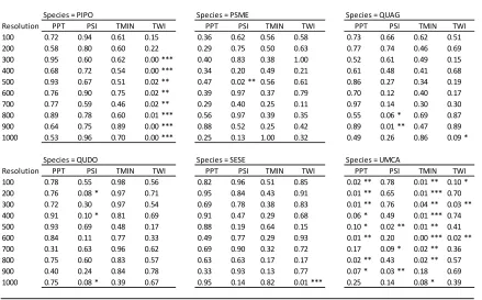
Table 2. Results of the paired t-tests between estimated parameter values of environmental covariates from true and fuzzed coordinates for each species. Each mini-table represents the species, the rows contain grain sizes, and the columns list the environmental variables. The cells within the tables list the corresponding p-values. Asterisks (*) indicate a statistically significant difference (* p<0.1, ** p<0.05, *** p<0.01). The abbreviations in the table follow

as: PPT, mean total yearly precipitation (1981-2010); PSI, potential solar irradiance

(calculated for the 183rd day (July 2nd) of 2014); TMIN, monthly mean of minimum daily

temperature (1981-2010); TWI, topographic wetness index. PIPO, Pinus ponderosa; PSME, Pseudotsuga menziesii; QUAG, Quercus Agrifolia; QUDO, Quercus douglasii; SESE,

Sequoia semprevirens; UMCA, Umbellularia californica.

Resolution

100 0.72 0.94 0.61 0.15 0.36 0.62 0.56 0.58 0.73 0.66 0.62 0.51

200 0.58 0.80 0.60 0.22 0.29 0.75 0.50 0.63 0.77 0.74 0.46 0.69

300 0.95 0.60 0.62 0.00 *** 0.40 0.83 0.38 1.00 0.52 0.61 0.49 0.15

400 0.68 0.72 0.54 0.00 *** 0.34 0.20 0.49 0.21 0.61 0.48 0.41 0.68

500 0.93 0.67 0.51 0.02 ** 0.47 0.02 ** 0.56 0.61 0.86 0.27 0.34 0.19

600 0.76 0.90 0.75 0.02 ** 0.39 0.97 0.37 0.79 0.70 0.12 0.40 0.17

700 0.77 0.59 0.46 0.02 ** 0.29 0.40 0.25 0.11 0.97 0.14 0.30 0.30

800 0.89 0.78 0.60 0.01 *** 0.56 0.97 0.39 0.35 0.55 0.06 * 0.69 0.87 900 0.64 0.75 0.89 0.00 *** 0.88 0.52 0.25 0.42 0.89 0.01 ** 0.47 0.89 1000 0.53 0.96 0.70 0.00 *** 0.25 0.13 1.00 0.32 0.49 0.26 0.86 0.09 *

Resolution

100 0.78 0.55 0.98 0.56 0.82 0.96 0.51 0.85 0.02 ** 0.78 0.01 ** 0.10 * 200 0.76 0.08 * 0.97 0.71 0.95 0.84 0.43 0.91 0.01 ** 0.65 0.01 *** 0.70 300 0.72 0.30 0.97 0.54 0.69 0.78 0.38 0.83 0.01 ** 0.76 0.04 ** 0.03 ** 400 0.91 0.10 * 0.81 0.69 0.91 0.47 0.29 0.68 0.06 * 0.49 0.01 *** 0.74 500 0.93 0.69 0.48 0.17 0.88 0.19 0.64 0.15 0.10 * 0.02 ** 0.01 ** 0.41 600 0.84 0.11 0.77 0.33 0.49 0.77 0.29 0.93 0.01 ** 0.20 0.00 *** 0.02 ** 700 0.31 0.63 0.96 0.62 0.69 0.90 0.32 0.72 0.17 0.09 * 0.02 ** 0.36 800 0.75 0.60 0.83 0.57 0.63 0.63 0.17 0.17 0.02 ** 0.43 0.02 ** 0.57 900 0.40 0.24 0.84 0.78 0.33 0.93 0.13 0.77 0.07 * 0.03 ** 0.18 0.69 1000 0.75 0.08 * 0.39 0.67 0.95 0.14 0.82 0.01 *** 0.25 0.14 0.08 * 0.39

Species = QUAG

PPT PSI TMIN TWI

Species = UMCA

PPT PSI TMIN TWI

Species = PIPO Species = PSME

PPT PSI TMIN TWI

Species = QUDO

PPT PSI TMIN TWI

Species = SESE

(26)

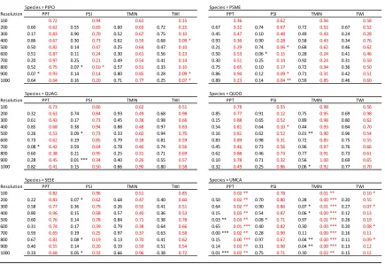
Table 3. Results of the paired t-tests between 100 m true coordinate models (assumed to be the most accurate) and all other grain sizes and coordinate types for each species. Black text indicates comparisons between the 100 m true coordinate model output compared to other grain sizes using true coordinates. Red text indicates comparisons between the 100 m true coordinate model output compared to the output of models using fuzzed coordinates. Each mini-table represents the species, the rows contain grain sizes, and the columns list the environmental variables. The cells within the tables list the corresponding p-values. Asterisks (*) indicate a statistically significant difference (* p<0.1, ** p<0.05, *** p<0.01).

Abbreviations in the table follow as: PPT, mean total yearly precipitation (1981-2010); PSI,

potential solar irradiance (calculated for the 183rd day (July 2nd) of 2014); TMIN, monthly

mean of minimum daily temperature (1981-2010); TWI, topographic wetness index. PIPO, Pinus ponderosa; PSME, Pseudotsuga menziesii; QUAG, Quercus agrifolia; QUDO,

Quercus douglasii; SESE, Sequoia sempervirens; UMCA, Umbellularia californica.

Resolution

100 0.72 0.94 0.61 0.15 0.36 0.62 0.56 0.58

200 0.60 0.62 0.55 0.65 0.60 0.63 0.72 0.25 0.67 0.32 0.74 0.67 0.72 0.52 0.67 0.52

300 0.17 0.83 0.90 0.70 0.52 0.67 0.75 0.10 0.45 0.47 0.10 0.48 0.49 0.43 0.24 0.28

400 0.86 0.67 0.30 0.73 0.62 0.59 0.68 0.09 * 0.93 0.36 0.90 0.28 0.58 0.43 0.34 0.76

500 0.50 0.82 0.14 0.47 0.25 0.64 0.47 0.10 0.21 0.29 0.74 0.06 * 0.68 0.62 0.46 0.62

600 0.51 0.87 0.11 0.24 0.30 0.61 0.56 0.23 0.50 0.53 0.06 * 0.15 0.28 0.24 0.41 0.46

700 0.20 0.97 0.25 0.21 0.49 0.54 0.41 0.14 0.30 0.51 0.25 0.14 0.92 0.24 0.31 0.59

800 0.52 0.75 0.07 * 0.10 * 0.57 0.51 0.33 0.10 0.75 0.65 0.10 0.17 0.72 0.34 0.36 0.50

900 0.07 * 0.93 0.14 0.14 0.80 0.85 0.28 0.09 * 0.86 0.94 0.12 0.09 * 0.71 0.31 0.42 0.51

1000 0.64 0.64 0.16 0.20 0.71 0.77 0.25 0.07 * 0.89 0.23 0.14 0.04 ** 0.59 0.85 0.46 0.60

Resolution

100 0.73 0.66 0.62 0.51 0.78 0.55 0.98 0.56

200 0.32 0.63 0.74 0.84 0.93 0.49 0.68 0.98 0.85 0.77 0.91 0.12 0.75 0.95 0.69 0.98

300 0.61 0.43 0.17 0.73 0.45 0.38 0.98 0.66 0.15 0.88 0.65 0.52 0.89 0.98 0.80 0.62

400 0.85 0.68 0.38 0.94 0.88 0.48 0.97 0.83 0.54 0.81 0.64 0.10 * 0.44 0.93 0.84 0.70

500 0.26 0.53 0.09 * 0.73 0.33 0.60 0.94 0.70 0.16 0.81 0.62 0.52 0.01 ** 0.90 0.96 0.54

600 0.73 0.62 0.19 0.85 0.79 0.38 0.81 0.59 0.83 0.89 0.98 0.31 0.72 0.85 0.75 0.55

700 0.08 * 0.42 0.59 0.64 0.78 0.40 0.74 0.56 0.45 0.46 0.73 0.56 0.96 0.97 0.76 0.66

800 0.60 0.38 0.21 0.95 0.25 0.31 0.71 0.69 0.62 0.88 0.46 0.73 0.77 0.91 0.73 0.61

900 0.28 0.45 0.01 *** 0.34 0.40 0.26 0.55 0.57 0.10 0.78 0.71 0.32 0.56 1.00 0.69 0.65

1000 0.82 0.41 0.15 0.50 0.66 0.90 0.80 0.58 0.32 0.49 0.25 0.86 0.06 * 0.92 0.77 0.70

Resolution

100 0.82 0.96 0.51 0.85 0.02 ** 0.78 0.01 ** 0.10 *

200 0.22 0.83 0.07 * 0.62 0.68 0.47 0.40 0.60 0.50 0.02 ** 0.70 0.80 0.28 0.00 *** 0.20 0.55

300 0.58 0.77 0.36 0.79 0.26 0.55 0.41 0.51 0.64 0.02 ** 0.90 0.86 0.07 * 0.01 *** 0.27 0.07 *

400 0.80 0.96 0.15 0.68 0.57 0.40 0.36 0.53 0.15 0.03 ** 0.54 0.87 0.06 * 0.00 *** 0.12 0.13

500 0.60 0.76 0.14 0.78 0.84 0.71 0.38 0.78 0.03 ** 0.03 ** 0.08 * 0.71 0.97 0.01 *** 0.26 0.19

600 0.31 0.74 0.17 0.39 0.79 0.38 0.64 0.66 0.65 0.01 *** 0.40 0.82 0.30 0.00 *** 0.20 0.08 *

700 0.93 0.69 0.19 0.25 0.97 0.37 0.63 0.58 0.00 *** 0.02 ** 0.28 0.90 0.11 0.00 *** 0.16 0.11

800 0.67 0.81 0.08 * 0.19 0.13 0.70 0.41 0.62 0.15 0.00 *** 0.97 0.67 0.04 ** 0.00 *** 0.11 0.09 *

900 0.40 0.55 0.14 0.20 0.19 0.59 0.51 0.54 0.14 0.02 ** 0.31 0.90 0.04 ** 0.00 *** 0.13 0.12

1000 0.33 0.68 0.05 * 0.32 0.66 0.96 0.38 0.72 0.01 *** 0.02 ** 0.75 0.71 0.30 0.02 ** 0.15 0.12

Species = SESE Species = UMCA PPT

PPT PSI

Species = PIPO Species = PSME

Species = QUAG Species = QUDO TWI

PSI TMIN TWI PPT PSI

PPT PSI TMIN TWI PPT PSI TMIN TWI

PSI TMIN TWI

(27)

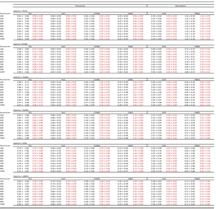
Table 4. Accuracy metric means and standard deviation for models using true and fuzz coordinate data models at each resolution for each species. Black indicates TRUE model. Red indicates FUZZ model. Bold indicates greater accuracy. Asterisks (*) indicate a

statistically significant difference (* p<0.1, ** p<0.05, *** p<0.01) in means of the accuracy metric between TRUE and FUZZ models for the species at the resolution. Abbreviations follow as: Occurrence accuracy metrics: AUC, area under curve; COMMISSION, false positive rate (type I error) ; OMISSION, false negative rate (type II error); TSS, true skill statistic. Abundance accuracy metrics: COR, Pearson correlation coefficient; RMSE, root

mean square error, units in square meters (m2). PIPO, Pinus ponderosa; PSME,

Pseudotsuga menziesii; QUAG, Quercus Agrifolia; QUDO, Quercus douglasii; SESE,

Sequoia semprevirens; UMCA, Umbellularia californica.

Resolution

100 0.51 ± 0.03 0.49 ± 0.04 0.83 ± 0.02 0.83 ± 0.02 0.25 ± 0.02 0.25 ± 0.01 0.24 ± 0.03 0.26 ± 0.04 0.14 ± 0.03 0.14 ± 0.03 1.22 ± 0.19 1.22 ± 0.19 200 0.51 ± 0.04 0.49 ± 0.05 0.83 ± 0.02 0.83 ± 0.02 0.25 ± 0.02 0.25 ± 0.01 0.25 ± 0.03 0.25 ± 0.04 0.14 ± 0.03 0.13 ± 0.03 1.22 ± 0.19 1.22 ± 0.19 300 0.50 ± 0.03 0.49 ± 0.05 0.83 ± 0.02 0.83 ± 0.02 0.25 ± 0.02 0.25 ± 0.01 0.25 ± 0.03 0.26 ± 0.04 0.14 ± 0.03 0.14 ± 0.03 1.22 ± 0.19 1.22 ± 0.19 400 0.50 ± 0.04 0.49 ± 0.05 0.83 ± 0.02 0.83 ± 0.02 0.25 ± 0.02 0.25 ± 0.01 0.25 ± 0.03 0.25 ± 0.04 0.14 ± 0.03 0.14 ± 0.03 1.22 ± 0.19 1.22 ± 0.19 500 0.50 ± 0.04 0.49 ± 0.05 0.83 ± 0.02 0.82 ± 0.02 0.25 ± 0.02 0.25 ± 0.01 0.25 ± 0.03 0.26 ± 0.04 0.14 ± 0.03 0.14 ± 0.03 1.22 ± 0.19 1.22 ± 0.19 600 0.51 ± 0.03 0.49 ± 0.05 0.83 ± 0.02 0.82 ± 0.02 0.25 ± 0.02 0.25 ± 0.01 0.24 ± 0.03 0.25 ± 0.04 0.14 ± 0.03 0.14 ± 0.03 1.22 ± 0.19 1.22 ± 0.19 700 0.50 ± 0.03 0.49 ± 0.04 0.83 ± 0.02 0.82 ± 0.02 0.25 ± 0.02 0.25 ± 0.01 0.25 ± 0.03 0.25 ± 0.04 0.14 ± 0.03 0.14 ± 0.03 1.22 ± 0.19 1.22 ± 0.19 800 0.50 ± 0.03 0.49 ± 0.05 0.83 ± 0.02 0.82 ± 0.02 0.26 ± 0.02 0.25 ± 0.01 0.25 ± 0.03 0.25 ± 0.05 0.14 ± 0.03 0.14 ± 0.03 1.22 ± 0.19 1.22 ± 0.19 900 0.50 ± 0.03 0.49 ± 0.04 0.83 ± 0.02 0.82 ± 0.02 0.25 ± 0.02 0.25 ± 0.01 0.25 ± 0.03 0.26 ± 0.05 0.14 ± 0.03 0.14 ± 0.03 1.22 ± 0.19 1.22 ± 0.19 1000 0.50 ± 0.04 0.50 ± 0.05 0.83 ± 0.02 0.82 ± 0.02 0.25 ± 0.02 0.25 ± 0.01 0.25 ± 0.03 0.25 ± 0.04 0.14 ± 0.04 0.14 ± 0.03 1.22 ± 0.19 1.22 ± 0.19

Resolution

100 0.58 ± 0.02 0.57 ± 0.03 0.87 ± 0.01 0.87 ± 0.01 0.24 ± 0.02 0.25 ± 0.02 0.18 ± 0.02 0.18 ± 0.02 0.30 ± 0.03 0.30 ± 0.04 3.72 ± 0.27 3.72 ± 0.31 200 0.58 ± 0.02 0.57 ± 0.03 0.87 ± 0.01 0.87 ± 0.01 0.24 ± 0.03 0.24 ± 0.03 0.18 ± 0.01 0.18 ± 0.02 0.30 ± 0.03 0.30 ± 0.04 3.71 ± 0.26 3.71 ± 0.31 300 0.58 ± 0.02 0.58 ± 0.03 0.87 ± 0.01 0.87 ± 0.01 0.24 ± 0.03 0.24 ± 0.03 0.18 ± 0.01 0.18 ± 0.01 0.30 ± 0.03 0.30 ± 0.04 3.71 ± 0.27 3.72 ± 0.31 400 0.58 ± 0.02 0.58 ± 0.03 0.87 ± 0.01 0.87 ± 0.01 0.24 ± 0.03 0.24 ± 0.02 0.18 ± 0.01 0.18 ± 0.01 0.31 ± 0.03 0.30 ± 0.03 3.70 ± 0.27 3.71 ± 0.31 500 0.58 ± 0.02 0.57 ± 0.02 0.87 ± 0.01 0.87 ± 0.01 0.24 ± 0.03 0.24 ± 0.02 0.18 ± 0.01 0.18 ± 0.01 0.31 ± 0.03 0.30 ± 0.04 3.71 ± 0.27 3.71 ± 0.31 600 0.58 ± 0.02 0.57 ± 0.03 0.87 ± 0.01 0.87 ± 0.01 0.24 ± 0.03 0.24 ± 0.03 0.18 ± 0.01 0.18 ± 0.01 0.32 ± 0.03 0.31 ± 0.03 3.70 ± 0.27 3.70 ± 0.31 700 0.59 ± 0.03 0.58 ± 0.03 0.87 ± 0.01 0.87 ± 0.01 0.24 ± 0.03 0.24 ± 0.03 0.18 ± 0.01 0.18 ± 0.01 0.32 ± 0.03 0.31 ± 0.04 3.69 ± 0.27 3.70 ± 0.31 800 0.58 ± 0.03 0.58 ± 0.04 0.87 ± 0.01 0.87 ± 0.01 0.24 ± 0.03 0.24 ± 0.03 0.18 ± 0.01 0.18 ± 0.02 0.32 ± 0.03 0.31 ± 0.03 3.69 ± 0.27 3.70 ± 0.31 900 0.59 ± 0.02 0.58 ± 0.03 0.87 ± 0.01 0.87 ± 0.01 0.24 ± 0.03 0.24 ± 0.03 0.18 ± 0.01 0.18 ± 0.01 0.31 ± 0.03 0.31 ± 0.03 3.70 ± 0.27 3.70 ± 0.31 1000 0.59 ± 0.03 0.58 ± 0.03 0.87 ± 0.01 0.87 ± 0.01 0.23 ± 0.03 0.24 ± 0.03 0.18 ± 0.01 0.18 ± 0.01 0.33 ± 0.03 0.32 ± 0.04 3.68 ± 0.27 3.70 ± 0.31

Resolution

100 0.49 ± 0.11 0.48 ± 0.09 0.83 ± 0.03 0.82 ± 0.03 0.26 ± 0.05 0.26 ± 0.05 0.25 ± 0.09 0.26 ± 0.07 0.34 ± 0.07 0.34 ± 0.08 0.66 ± 0.24 0.66 ± 0.24 200 0.49 ± 0.11 0.48 ± 0.10 0.83 ± 0.03 0.83 ± 0.04 0.26 ± 0.05 0.26 ± 0.05 0.25 ± 0.09 0.26 ± 0.09 0.34 ± 0.07 0.34 ± 0.08 0.66 ± 0.24 0.66 ± 0.24 300 0.48 ± 0.10 0.49 ± 0.10 0.83 ± 0.02 0.82 ± 0.03 0.26 ± 0.05 0.26 ± 0.05 0.25 ± 0.09 0.26 ± 0.07 0.34 ± 0.07 0.34 ± 0.08 0.66 ± 0.24 0.66 ± 0.24 400 0.48 ± 0.11 0.47 ± 0.09 0.83 ± 0.02 0.82 ± 0.03 0.27 ± 0.05 0.26 ± 0.04 0.24 ± 0.10 0.27 ± 0.08 0.34 ± 0.07 0.34 ± 0.08 0.66 ± 0.24 0.66 ± 0.24 500 0.47 ± 0.09 0.47 ± 0.09 0.83 ± 0.02 0.82 ± 0.04 0.25 ± 0.06 0.26 ± 0.05 0.27 ± 0.08 0.27 ± 0.07 0.34 ± 0.06 0.33 ± 0.08 0.66 ± 0.24 0.66 ± 0.24 600 0.47 ± 0.08 0.49 ± 0.10 0.83 ± 0.02 0.82 ± 0.03 0.26 ± 0.04 0.26 ± 0.04 0.26 ± 0.07 0.25 ± 0.09 0.34 ± 0.07 0.34 ± 0.08 0.66 ± 0.24 0.66 ± 0.24 700 0.49 ± 0.11 0.48 ± 0.11 0.83 ± 0.03 0.82 ± 0.03 0.26 ± 0.05 0.26 ± 0.05 0.25 ± 0.10 0.26 ± 0.09 0.34 ± 0.07 0.34 ± 0.08 0.66 ± 0.24 0.66 ± 0.24 800 0.46 ± 0.09 0.49 ± 0.11 0.83 ± 0.03 0.82 ± 0.03 0.28 ± 0.05 0.26 ± 0.05 0.26 ± 0.07 0.25 ± 0.09 0.34 ± 0.07 0.33 ± 0.07 0.66 ± 0.24 0.66 ± 0.24 900 0.47 ± 0.08 0.47 ± 0.10 0.83 ± 0.03 0.82 ± 0.03 0.27 ± 0.05 0.26 ± 0.05 0.27 ± 0.06 0.26 ± 0.07 0.34 ± 0.08 0.34 ± 0.08 0.66 ± 0.24 0.66 ± 0.24 1000 0.47 ± 0.08 0.48 ± 0.10 0.83 ± 0.03 0.82 ± 0.04 0.26 ± 0.05 0.26 ± 0.05 0.28 ± 0.07 0.26 ± 0.07 0.34 ± 0.07 0.34 ± 0.08 0.66 ± 0.24 0.66 ± 0.24

Resolution

100 0.65 ± 0.08 0.66 ± 0.07 0.89 ± 0.02 0.89 ± 0.03 0.20 ± 0.02 0.19 ± 0.03 0.15 ± 0.07 0.15 ± 0.06 0.37 ± 0.03 0.36 ± 0.04 0.27 ± 0.03 0.27 ± 0.03 200 0.65 ± 0.07 0.65 ± 0.06 0.89 ± 0.02 0.89 ± 0.03 0.19 ± 0.02 0.19 ± 0.03 0.15 ± 0.06 0.15 ± 0.06 0.37 ± 0.03 0.36 ± 0.03 0.27 ± 0.03 0.27 ± 0.03 300 0.65 ± 0.07 0.66 ± 0.06 0.90 ± 0.02 0.89 ± 0.03 0.19 ± 0.01 0.19 ± 0.03 0.15 ± 0.06 0.15 ± 0.06 0.37 ± 0.04 0.36 ± 0.04 0.27 ± 0.03 0.27 ± 0.03 400 0.65 ± 0.06 0.66 ± 0.06 0.89 ± 0.02 0.89 ± 0.03 0.19 ± 0.02 0.20 ± 0.03 0.16 ± 0.06 0.15 ± 0.06 0.37 ± 0.04 0.36 ± 0.04 0.27 ± 0.03 0.27 ± 0.03 500 0.65 ± 0.07 0.66 ± 0.06 0.89 ± 0.02 0.89 ± 0.03 0.19 ± 0.02 0.19 ± 0.03 0.16 ± 0.07 0.14 ± 0.06 0.37 ± 0.03 0.36 ± 0.04 0.27 ± 0.03 0.27 ± 0.03 600 0.66 ± 0.07 0.66 ± 0.06 0.90 ± 0.02 0.89 ± 0.03 0.19 ± 0.02 0.19 ± 0.03 0.15 ± 0.06 0.15 ± 0.06 0.37 ± 0.04 0.36 ± 0.04 0.27 ± 0.03 0.27 ± 0.03 700 0.65 ± 0.07 0.65 ± 0.08 0.89 ± 0.02 0.89 ± 0.03 0.19 ± 0.02 0.19 ± 0.04 0.15 ± 0.07 0.15 ± 0.07 0.37 ± 0.04 0.35 ± 0.04 0.27 ± 0.03 0.27 ± 0.03 800 0.64 ± 0.07 0.67 ± 0.07 0.89 ± 0.02 0.89 ± 0.03 0.20 ± 0.02 0.19 ± 0.03 0.16 ± 0.06 0.14 ± 0.06 0.37 ± 0.03 0.36 ± 0.03 0.27 ± 0.03 0.27 ± 0.03 900 0.66 ± 0.08 0.66 ± 0.06 0.90 ± 0.02 0.89 ± 0.03 0.19 ± 0.02 0.19 ± 0.03 0.15 ± 0.08 0.15 ± 0.06 0.37 ± 0.04 0.35 ± 0.04 0.27 ± 0.03 0.27 ± 0.03 1000 0.66 ± 0.08 0.65 ± 0.06 0.89 ± 0.02 0.89 ± 0.03 0.19 ± 0.02 0.19 ± 0.03 0.16 ± 0.08 0.15 ± 0.06 0.37 ± 0.04 0.35 ± 0.03 0.27 ± 0.03 0.27 ± 0.03

Resolution

100 0.73 ± 0.05 0.72 ± 0.08 0.93 ± 0.03 0.92 ± 0.04 0.13 ± 0.04 0.13 ± 0.06 0.14 ± 0.06 0.15 ± 0.08 0.24 ± 0.09 0.25 ± 0.07 6.63 ± 2.84 6.49 ± 3.10 200 0.73 ± 0.06 0.71 ± 0.09 0.93 ± 0.03 0.93 ± 0.04 0.13 ± 0.05 0.13 ± 0.06 0.14 ± 0.06 0.16 ± 0.08 0.24 ± 0.10 0.27 ± 0.05 6.63 ± 2.84 6.45 ± 3.13 300 0.74 ± 0.05 0.71 ± 0.08 0.93 ± 0.03 0.92 ± 0.04 0.13 ± 0.05 0.13 ± 0.06 0.14 ± 0.06 0.16 ± 0.09 0.25 ± 0.10 0.26 ± 0.07 6.61 ± 2.84 6.45 ± 3.12 400 0.73 ± 0.06 0.71 ± 0.08 0.93 ± 0.03 0.93 ± 0.04 0.13 ± 0.05 0.13 ± 0.06 0.14 ± 0.06 0.16 ± 0.08 0.24 ± 0.09 0.28 ± 0.07 6.63 ± 2.83 6.43 ± 3.14 500 0.74 ± 0.05 0.74 ± 0.06 0.93 ± 0.03 0.93 ± 0.04 0.13 ± 0.05 0.12 ± 0.06 0.13 ± 0.06 0.14 ± 0.07 0.24 ± 0.10 0.28 ± 0.08 6.61 ± 2.87 6.42 ± 3.14 600 0.74 ± 0.04 0.72 ± 0.09 0.93 ± 0.03 0.93 ± 0.04 0.13 ± 0.05 0.13 ± 0.07 0.13 ± 0.05 0.15 ± 0.08 0.24 ± 0.10 0.28 ± 0.08 6.63 ± 2.85 6.42 ± 3.16 700 0.74 ± 0.05 0.71 ± 0.10 0.93 ± 0.03 0.93 ± 0.04 0.13 ± 0.05 0.13 ± 0.06 0.13 ± 0.06 0.16 ± 0.09 0.26 ± 0.09 0.27 ± 0.06 6.58 ± 2.84 6.43 ± 3.16 800 0.72 ± 0.07 0.70 ± 0.09 0.93 ± 0.03 0.93 ± 0.04 0.14 ± 0.05 0.14 ± 0.05 0.15 ± 0.07 0.16 ± 0.08 0.24 ± 0.10 0.27 ± 0.09 6.62 ± 2.86 6.46 ± 3.14 900 0.73 ± 0.05 0.70 ± 0.09 0.93 ± 0.03 0.93 ± 0.04 0.13 ± 0.05 0.13 ± 0.06 0.14 ± 0.06 0.17 ± 0.10 0.25 ± 0.10 0.26 ± 0.07 6.61 ± 2.85 6.45 ± 3.17 1000 0.71 ± 0.07 0.70 ± 0.09 0.93 ± 0.03 0.93 ± 0.03 0.14 ± 0.05 0.14 ± 0.05 0.15 ± 0.07 0.17 ± 0.08 0.24 ± 0.10 0.27 ± 0.08 6.62 ± 2.86 6.44 ± 3.15

Resolution

100 0.40 ± 0.06 0.39 ± 0.06 0.79 ± 0.03 0.79 ± 0.03 0.28 ± 0.02 0.28 ± 0.03 0.32 ± 0.07 0.34 ± 0.08 0.18 ± 0.03 0.18 ± 0.03 0.17 ± 0.05 0.17 ± 0.05 200 0.41 ± 0.07 0.42 ± 0.08 0.79 ± 0.03 0.80 ± 0.04 0.28 ± 0.02 0.27 ± 0.03 0.31 ± 0.08 0.31 ± 0.09 0.18 ± 0.03 0.17 ± 0.03 0.17 ± 0.05 0.17 ± 0.05 300 0.43 ± 0.08 0.40 ± 0.07 0.79 ± 0.04 0.79 ± 0.03 0.28 ± 0.02 0.28 ± 0.02 0.29 ± 0.08 0.31 ± 0.08 0.18 ± 0.03 0.17 ± 0.03 0.17 ± 0.05 0.17 ± 0.05 400 0.42 ± 0.06 0.43 ± 0.07 0.79 ± 0.03 0.79 ± 0.03 0.28 ± 0.02 0.28 ± 0.03 0.30 ± 0.07 0.29 ± 0.08 0.18 ± 0.03 0.18 ± 0.03 0.17 ± 0.05 0.17 ± 0.05 500 0.45 ± 0.05 0.41 ± 0.08 0.80 ± 0.03 0.79 ± 0.04 0.29 ± 0.02 0.28 ± 0.03 0.26 ± 0.05 0.31 ± 0.09 0.17 ± 0.02 0.18 ± 0.03 0.17 ± 0.05 0.17 ± 0.05 600 0.43 ± 0.07 0.40 ± 0.08 0.80 ± 0.03 0.79 ± 0.03 0.29 ± 0.02 0.27 ± 0.02 0.29 ± 0.08 0.32 ± 0.10 0.18 ± 0.03 0.18 ± 0.03 0.17 ± 0.05 0.17 ± 0.05 700 0.44 ± 0.07 0.43 ± 0.06 0.80 ± 0.03 0.80 ± 0.03 0.29 ± 0.03 0.28 ± 0.02 0.27 ± 0.07 0.28 ± 0.08 0.18 ± 0.04 0.17 ± 0.03 0.17 ± 0.05 0.17 ± 0.05 800 0.43 ± 0.06 0.42 ± 0.07 0.79 ± 0.03 0.79 ± 0.03 0.29 ± 0.03 0.28 ± 0.03 0.28 ± 0.06 0.30 ± 0.08 0.17 ± 0.04 0.17 ± 0.04 0.17 ± 0.05 0.17 ± 0.05 900 0.45 ± 0.07 0.43 ± 0.08 0.80 ± 0.03 0.80 ± 0.03 0.28 ± 0.03 0.28 ± 0.03 0.27 ± 0.07 0.29 ± 0.09 0.18 ± 0.03 0.18 ± 0.03 0.17 ± 0.05 0.17 ± 0.05 1000 0.45 ± 0.07 0.42 ± 0.07 0.80 ± 0.03 0.80 ± 0.03 0.29 ± 0.03 0.28 ± 0.02 0.26 ± 0.06 0.29 ± 0.07 0.18 ± 0.04 0.17 ± 0.03 0.17 ± 0.05 0.17 ± 0.05

COR RMSE Species =PSME

Occurance

AUC COMIS OMIS

Abundance Species = PIPO

TSS

TSS AUC COMIS OMIS COR RMSE

COR RMSE

AUC COMIS OMIS COR RMSE

RMSE Species = QUAG

Species = QUDO

Species = SESE

Species = UMCA

TSS AUC COMIS OMIS COR

TSS

(28)

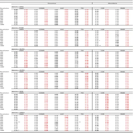
Table 5. Accuracy metric means for true and fuzz coordinate models at each resolution for each species. Black indicates TRUE model. Red indicates FUZZ model. Bold indicates greater accuracy. Asterisks (*) indicate a statistically significant difference (* p<0.1, ** p<0.05, *** p<0.01) in means of the accuracy metric between the 100 m TRUE model and the corresponding TRUE or FUZZ model for the species at the resolution. Please refer to Table 3 for standard errors associated with accuracy metrics.Abbreviations follow as:

Occurrence accuracy metrics: AUC, area under curve; COMMISSION, false positive rate (type I error); OMISSION, false negative rate (type II error); TSS, true skill statistic. Abundance accuracy metrics: COR, Pearson correlation coefficient; RMSE, root mean

square error, units in square meters (m2). PIPO, Pinus ponderosa; PSME, Pseudotsuga

menziesii; QUAG, Quercus Agrifolia; QUDO, Quercus douglasii; SESE, Sequoia

semprevirens; UMCA, Umbellularia californica.

Resolution

100 0.24 0.26 0.25 0.25 0.83 0.83 0.51 0.49 0.14 0.14 1.22 1.22

200 0.25 0.25 0.25 0.25 0.83 0.83 0.51 0.49 0.14 0.13 1.22 1.22

300 0.25 0.26 0.25 0.25 0.83 0.83 0.50 0.49 0.14 0.14 1.22 1.22

400 0.25 0.25 0.25 0.25 0.83 0.83 0.50 0.49 0.14 0.14 1.22 1.22

500 0.25 0.26 0.25 0.25 0.83 0.82 0.50 0.49 0.14 0.14 1.22 1.22

600 0.24 0.25 0.25 0.25 0.83 0.82 0.51 0.49 0.14 0.14 1.22 1.22

700 0.25 0.25 0.25 0.25 0.83 0.82 0.50 0.49 0.14 0.14 1.22 1.22

800 0.25 0.25 0.26 0.25 0.83 0.82 0.50 0.49 0.14 0.14 1.22 1.22

900 0.25 0.26 0.25 0.25 0.83 0.82 0.50 0.49 0.14 0.14 1.22 1.22

1000 0.25 0.25 0.25 0.25 0.83 0.82 0.50 0.50 0.14 0.14 1.22 1.22

Resolution

100 0.18 0.18 0.24 0.25 0.87 0.87 0.58 0.57 0.30 0.30 3.72 3.72

200 0.18 0.18 0.24 0.24 0.87 0.87 0.58 0.57 0.30 0.30 3.71 3.71

300 0.18 0.18 0.24 0.24 0.87 0.87 0.58 0.58 0.30 0.30 3.71 3.72

400 0.18 0.18 0.24 0.24 0.87 0.87 0.58 0.58 0.31 0.30 3.70 3.71

500 0.18 0.18 0.24 0.24 0.87 0.87 0.58 0.57 0.31 0.30 3.71 3.71

600 0.18 0.18 0.24 0.24 0.87 0.87 0.58 0.57 0.32 0.31 3.70 3.70

700 0.18 0.18 0.24 0.24 0.87 0.87 0.59 0.58 0.32 * 0.31 3.69 3.70

800 0.18 0.18 0.24 0.24 0.87 0.87 0.58 0.58 0.32 0.31 3.69 3.70

900 0.18 0.18 0.24 0.24 0.87 0.87 0.59 0.58 0.31 0.31 3.70 3.70

1000 0.18 0.18 0.23 0.24 0.87 0.87 0.59 0.58 0.33 ** 0.32 3.68 3.70

Resolution

100 0.25 0.26 0.26 0.26 0.83 0.82 0.49 0.48 0.34 0.34 0.66 0.66

200 0.25 0.26 0.26 0.26 0.83 0.83 0.49 0.48 0.34 0.34 0.66 0.66

300 0.25 0.26 0.26 0.26 0.83 0.82 0.48 0.49 0.34 0.34 0.66 0.66

400 0.24 0.27 0.27 0.26 0.83 0.82 0.48 0.47 0.34 0.34 0.66 0.66

500 0.27 0.27 0.25 0.26 0.83 0.82 0.47 0.47 0.34 0.33 0.66 0.66

600 0.26 0.25 0.26 0.26 0.83 0.82 0.47 0.49 0.34 0.34 0.66 0.66

700 0.25 0.26 0.26 0.26 0.83 0.82 0.49 0.48 0.34 0.34 0.66 0.66

800 0.26 0.25 0.28 0.26 0.83 0.82 0.46 0.49 0.34 0.33 0.66 0.66

900 0.27 0.26 0.27 0.26 0.83 0.82 0.47 0.47 0.34 0.34 0.66 0.66

1000 0.28 0.26 0.26 0.26 0.83 0.82 0.47 0.48 0.34 0.34 0.66 0.66

Resolution

100 0.15 0.15 0.20 0.19 0.89 0.89 0.65 0.66 0.37 0.36 0.27 0.27

200 0.15 0.15 0.19 0.19 0.89 0.89 0.65 0.65 0.37 0.36 0.27 0.27

300 0.15 0.15 0.19 0.19 0.90 0.89 0.65 0.66 0.37 0.36 0.27 0.27

400 0.16 0.15 0.19 0.20 0.89 0.89 0.65 0.66 0.37 0.36 0.27 0.27

500 0.16 0.14 0.19 0.19 0.89 0.89 0.65 0.66 0.37 0.36 0.27 0.27

600 0.15 0.15 0.19 0.19 0.90 0.89 0.66 0.66 0.37 0.36 0.27 0.27

700 0.15 0.15 0.19 0.19 0.89 0.89 0.65 0.65 0.37 0.35 0.27 0.27

800 0.16 0.14 0.20 0.19 0.89 0.89 0.64 0.67 0.37 0.36 0.27 0.27

900 0.15 0.15 0.19 0.19 0.90 0.89 0.66 0.66 0.37 0.35 0.27 0.27

1000 0.16 0.15 0.19 0.19 0.89 0.89 0.66 0.65 0.37 0.35 0.27 0.27

Resolution

100 0.14 0.15 0.13 0.13 0.93 0.92 0.73 0.72 0.24 0.25 6.63 6.49

200 0.14 0.16 0.13 0.13 0.93 0.93 0.73 0.71 0.24 0.27 6.63 6.45

300 0.14 0.16 0.13 0.13 0.93 0.92 0.74 0.71 0.25 0.26 6.61 6.45

400 0.14 0.16 0.13 0.13 0.93 0.93 0.73 0.71 0.24 0.28 6.63 6.43

500 0.13 0.14 0.13 0.12 0.93 0.93 0.74 0.74 0.24 0.28 6.61 6.42

600 0.13 0.15 0.13 0.13 0.93 0.93 0.74 0.72 0.24 0.28 6.63 6.42

700 0.13 0.16 0.13 0.13 0.93 0.93 0.74 0.71 0.26 0.27 6.58 6.43

800 0.15 0.16 0.14 0.14 0.93 0.93 0.72 0.70 0.24 0.27 6.62 6.46

900 0.14 0.17 0.13 0.13 0.93 0.93 0.73 0.70 0.25 0.26 6.61 6.45

1000 0.15 0.17 0.14 0.14 0.93 0.93 0.71 0.70 0.24 0.27 6.62 6.44

Resolution

100 0.32 0.34 0.28 0.28 0.79 0.79 0.40 0.39 0.18 0.18 0.17 0.17

200 0.31 0.31 0.28 0.27 0.79 0.80 0.41 0.42 0.18 0.17 0.17 0.17

300 0.29 0.31 0.28 0.28 0.79 0.79 0.43 0.40 0.18 0.17 0.17 0.17

400 0.30 0.29 0.28 0.28 0.79 0.79 0.42 0.43 0.18 0.18 0.17 0.17

500 0.26 ** 0.31 0.29 0.28 0.80 0.79 0.45 ** 0.41 0.17 0.18 0.17 0.17

600 0.29 0.32 0.29 0.27 0.80 0.79 0.43 0.40 0.18 0.18 0.17 0.17

700 0.27 0.28 0.29 0.28 0.80 0.80 0.44 0.43 0.18 0.17 0.17 0.17

800 0.28 0.30 0.29 0.28 0.79 0.79 0.43 0.42 0.17 0.17 0.17 0.17

900 0.27 0.29 0.28 0.28 0.80 0.80 0.45 * 0.43 0.18 0.18 0.17 0.17

1000 0.26 * 0.29 0.29 0.28 0.80 0.80 0.45 * 0.42 0.18 0.17 0.17 0.17

Occurance Abundance

Species = PIPO

OMIS COMIS AUC TSS COR RMSE

Species =PSME

RMSE Species = QUAG

OMIS COMIS AUC TSS COR

Species = UMCA

Species = SESE

(29)

REFERENCES

Allouche, O., Tsoar, A., & Kadmon, R. (2006) Assessing the accuracy of species distribution models: prevalence, kappa and true skill statistic (TSS). Journal of Applied Ecology 43: 1223–1232.

Augustin N.H., M.A. Mugglestone & S.T. Buckland. 1996. An autologistic model for the spatial distribution of wildlife. Journal of Applied Ecology 33: 339-347.

Barton, K. 2014. MuMIn: Multi-model inference. R package version 1.10.5. http://CRAN.R-project.org/package=MuMIn

Beven, K.J. & M.J. Kirby. 1979. A physically based, variable contributing area model of basin hydrology. Hydrological Sciences 24: 43-69.

Bivand, R. 2005. spdep: spatial dependence: weighting schemes, statistics and models. - R package version 0.3- 17.

Brand, G. 2004. Forest Inventory and Analysis sampling hexagons. FIA fact sheet series. Available from http://fia.fs.fed.us/library/

fact-sheets/datacollections/Sampling_hexagons.pdf [cited 11 April 2005].

Brockwell, P. J. & R.A. Davis. 1996. Introduction to time-series and forecasting. John Wiley & Sons

Byrt, T., Bishop, J. & Carlin, J.B. (1993) Bias, prevalence and kappa. Journal of Clinical

Epidemiology, 46, 423–429.

Cicchetti, D.V. & Feinstein, A.R. (1990) High agreement but low kappa. II. Resolving the paradoxes. Journal of Clinical Epidemiology, 43, 551–558.

Cohen, J. (1960) A coefficient of agreement of nominal scales. Educational and

Psychological Measurement, 20, 37–46.

Coulston, J.W., Reams, G.A., McRoberts, R.E., Smith, W.B. (2004) Practical considerations when using perturbed forest inventory plot locations to develop spatial models: a case study. In: McRoberts, R.E.; Reams, G.A.; VanDeusen, P.C.; McWilliams, W.H., eds. 2006. Proceedings of the sixth annual forest inventory and analysis symposium; 2004 September 21-24; Denver, CO. Gen. Tech. Rep. WO-70. Washington, D.C.: U.S. Department of Agriculture, Forest Service. 126 p.

Coulston, J.W., Riitters, K.H., McRoberts, R.E., Reams, G.A., & Smith, W.D. (2006) True versus perturbed forest inventory plot locations for modeling: a simulation study. Can J

(30)

Daly, C., R.P. Neilson, & D.L. Phillips. 1994. A Statistical-Topographic Model for Mapping Climatological Precipitation over Mountainous Terrain. J. Appl. Meteor. 33: 40-158.

Dolanc, C.R., Safford, H.D., Dobrowski, S.Z. & Thorne, J.H. (2014) Twentieth century shifts in abundance and composition of vegetation types of the Sierra Nevada, CA, US.

Applied Vegetation Science, 17, 442–455.

Dungan, J.L., Perry, J.N., Dale, M.R.T, Legendre, P., Citron-Pousty S., Fortin, M.J., Miriti, J.M., & Rosenberg, M.S. (2002) A balanced view of scale in spatial statistical analysis.

Ecography 25: 626–640.

Duong, Q.P. 1984. On the choice of the order of autoregressive models: a ranking and selection approach, J. Time Series Anal. 5: 145-157.

Elith, J. & Leathwick, J.R. (2009) Species Distribution Models: Ecological Explanation and Prediction Across Space and Time. Annual Review of Ecology, Evolution, and

Systematics 40: 677-697.

Fei, S. & Steiner, K.C. (2007) Evidence for Increasing Red Maple Abundance in the Eastern United States. Forest Science 53: 473-477.

Flint, L.E. & A.L. Flint. 2012. Downscaling future climate scenarios to fine scales for hydrologic and ecological modeling and analysis. Ecological Processes 1: 1-15.

Franklin, J., Davis, F.W., Ikegami, M., Syphard, A.D., Flint, L.E., Flint, A.L., & Hannah, L. (2013) Modeling plant species distributions under future climates: how fine scale do climate projections need to be? Global Change Biology 19: 473-483.

Gesch, D.B. 2007. The National Elevation Dataset, in Maune, D., ed., Digital Elevation Model Technologies and Applications: The DEM User’s Manual, 2nd Edition: Bethesda, Maryland, American Society for Photogrammetry and Remote Sensing, p. 99-118.

Gesch, D., M. Oimoen, S. Greenlee, C. Nelson, M. Steuck, & D. Tyler. 2002. The National Elevation Dataset. Photogrammetric Engineering and Remote Sensing 68: 5-11.

Gibson, J., Moisen, G., Frescino, T., & Edwards Jr., T.C. (2013) Using Publicly Available Forest Inventory Data in Climate-Based Models of Tree Species Distribution: Examining Effects of True Versus Altered Location Coordinates. Ecosystems 17: 43-53.

Gumpertz M.L., J.M. Graham J.B. Ristaino. 1997. Autologistic model of spatial pattern of Phytophthora epidemic in bell pepper: effects of soil variables on disease

(31)

Harris, R.B. (1999) Abundance and characteristics of snags in western Montana forests. Gen Tech. Rep. RMRS-GTR-31. Ogden, UT: U.S. Department of Agriculture, Forest Service, Rocky Mountain Research Station. 19 p.

Hijmans, R.J. 2012. Raster: Geographic analysis and modeling with raster data. R package version 2.3-0. http://CRAN.R-project.org/package=raster

Iverson, L.R. & Prasad, A.M. (1998) Predicting Abundance of 80 Tree Species Following Climate Change in the Eastern United States. Ecological Monographs 68: 465-485.

Iverson, L.R., Prasad, A.M., 2002. Potential redistribution of tree species habitat under five climate change scenarios in the eastern U.S. Forest Ecology and Management 155, 205– 222.

Lantz, C.A. & Nebenzahl, E. (1996) Behavior and interpreta- tion of the k statistic: resolution of two paradoxes. Journal of Clinical Epidemiology, 49, 431–434.

Manel, S., Williams, H.C. & Ormerod, S.J. (2001) Evaluating presence–absence models in ecology: the need to account for prevalence. Journal of Applied Ecology, 38, 921–931.

McPherson, J.M., Jetz, W. & Rogers, D.J. (2004) The effects of species’ range sizes on the accuracy of distribution models: ecological phenomenon or statistical artefact? Journal of

Applied Ecology, 41, 811–823.

McRoberts, R.E., Holden, G.R., Nelson, M.D., Liknes, G.C., Moser, W.K., Lister, A.J., King, S.L., LaPoint, E.B., Coulston, J.W., Smith, W.B., & Reams, G.A. (2005) Estimating and circumventing the effects of perturbing and swapping inventory plot locations. J For 103: 275–279.

Morin, R.S., Gottschalk, K.W., & Liebhold, A.M. (2003) Potential susceptibility of eastern forests to Sudden Oak Death, Phytophthora ramorum. 2003 forest health monitoring working group meeting. http://www.fhm.fs.fed.us/posters/posters03/ sod.pdf. (20 May 2005).

Myers, N. & Mittermeier, R. (2000) Biodiversity hotspots for conservation priorities. Nature, 403, 853–858.

Phillips, S.J., R.P. Anderson, R.E. Schapire, (2006) Maximum entropy modeling of species geographic distributions. Ecological Modelling 190. 231-259.

(32)

R Core Team (2013). R: A language and environment for statistical computing. R Foundation for Statistical Computing, Vienna, Austria. ISBN 3-900051-07-0, URL http://R-project.org/.

Reams, G.A., Smith, W.D., Hansen, M.H., Bechtold, W.A., Roesch, F., & Moisen, G.G. (2005) The forest inventory and analysis sampling frame. In The enhanced forest inventory and analysis program: national sampling design and estimation procedures.

Edited by W.A. Bechtold and P.L. Patterson. USDA For. Serv. Gen. Tech. Rep. SRS-80.

pp. 11–26.

Rich, P.M., R. Dubayah, W.A. Hetrick, & S.C. Saving. 1994. Using Viewshed Models to Calculate Intercepted Solar Radiation: Applications in Ecology. American Society for

Photogrammetry and Remote Sensing Technical Papers. 524-529.

Rich, P.M. & P. Fu. 2000. Topoclimatic Habitat Models. Proceedings of the Fourth

International Conference on Integrating GIS and Environmental Modeling.

Serra-Diaz, J.M., Franklin, J., Dillon, W.W., Syphard, A.D., Davis, A.W., Meentemeyer, R.K. (2015) California forests show early indications of both range shifts and local persistence under climate change. Global Ecology and Biogeography 25: 164-175.

Thorne, J.H., Morgan, B.J. & Kennedy, J.A. (2008) Vegetation change over sixty years in the

central Sierra Nevada, Califor- nia, USA. Madroño, 55, 223–237.

Tobalske, C. (2002) Effects of spatial scale on the predictive ability of habitat models for the Green Woodpecker in Switzerland. In Scott, J. M., Heglund, P. J., Mor- rison, M. L. et al.

(Eds.) Predicting Species Occurrences: Issues of Accuracy and Scale. Covelo, CA: Island Press, pp. 197–204.

VanDerWal, J., Shoo, L.P., Graham, C., & Williams, S.E. (2009) Selecting pseudo-absence data for presence only distribution modeling: How far should you stray from what you know? Ecological Modeling, 220, 589-594.

Woodall C.W., Oswalt C.M., Westfall J.A., Perry C.H., Nelson M.D., & Finley A.O. (2009) An indicator of tree migration in forests of the eastern United States. Forest Ecology and