Transactions, SMiRT-25 Charlotte, NC, USA, August 4-9, 2019
Division III
VALIDATION AND DETERMINATION OF SIGNIFICANT SIMULATION
PARAMETERS USING THE SMOOTHED PARTICLE HYDRODYNAMIC
CODE NEUTRINO
Emerald Ryan1, Steven Prescott2, Matthieu Andre3, Philippe Bardet4, Niels Montanari5, and Ramprasad Sampath6
1 INL Graduate Fellow, Idaho National Laboratory, Idaho Falls, ID, USA ([email protected]) 2 Software Engineer, Idaho National Laboratory, Idaho Falls, ID, USA
3 Research Professor, George Washington University, Washington, DC, USA 4 Associate Professor, George Washington University, Washington, DC, USA 5 Simulation Software Engineer, Centroid Lab, Los Angeles, CA, USA 6 Director of Research, Centroid Lab, Los Angeles, CA, USA
ABSTRACT
In recent years there has been an increase in flooding concern to nuclear power plants; thus, tools to reduce the cost of mitigation efforts are valuable to industry. Simulating flooding events is achieved through different methods and at varied levels of detail. However, these simulations must be able to match application conditions, which requires code validation as well as knowledge of which parameters affect the accuracy of the simulation. To validate and determine the significant parameters for these tools, a sloshing experiment was conducted at the George Washington University and then simulated with the smoothed particle hydrodynamic code Neutrino. The simulation setup was constructed to match the experiment as closely as possible, and the end-wall pressure results were analysed. The 90% and 50% end-wall pressure bounds were compared along with the pressure impulse. The simulation bounds fell mostly within the experimental bounds, with exceptions in insignificant low-pressure areas, such as at the beginning (~40% difference) and the end of the cycle (~40% difference). Another exception was seen at a point in the peak pressure (~75% difference). The simulated pressure impulse matched the experiments well and was within 10%. Additionally, seven parameters were qualitatively assessed and then investigated to determine their significance. The parameters’ significance was determined by sampling five values across the parameters’ range using the Risk Analysis Virtual Environment, then comparing the average pressure for each run. All seven parameters were identified as having some significance. However, the particle size, interaction-radius to particle-size ratio, and fluid settling seem to have a greater effect due to the larger fluctuation of the results. Now that the significant parameters are identified, further research is being done to quantify the significance of each parameter.
INTRODUCTION
validation. Additionally, there are many parameters for these simulations, so it is important to know which parameters are the most significant and how they affect accuracy and would relate to a real scenario.
To validate and determine significant parameters, an oscillation experiment was constructed and then simulated in the smoothed particle hydrodynamic (SPH) code Neutrino. The following sections describe both the experimental and simulation setups, the investigated parameters and methodology, and the results of the validation and determination of significant parameters.
EXPERIMENTAL SETUP
A large-scale oscillating tank was designed and constructed at the George Washington University. The tank measures 5.951 m long × 1.2 m high × 2.468 m wide. The tank is constructed of a steel frame and acrylic walls and bottom. The tank is oscillated through a sine-forcing function using a hydraulic actuator capable of amplitudes up to 0.25 m and velocities up to 0.5 m/s. Additionally, a pressure transducer is located at the end-wall of the tank, 0.1016 m above the tank bottom, to measure the pressure from wave impacts.
The experiment for the end-wall pressure measurement consisted of a water depth of 0.1524 m. The forcing function had a 0.1016 m amplitude, with a 0.11 Hz frequency. The experiment ran for 60 cycles and was repeated four times, with minor variations to account for some uncertainties. Two of the runs were identical; one run varied the depth by adding a precisely measured volume of water to the tank, and the last run varied the forcing function amplitude. Table 1 shows the variations on the four experimental model runs.
Table 1: Experimental model run variations.
Run Water Depth (m) Frequency (Hz) Amplitude (m) Variation
1 0.1524 0.11 0.1016 Reference run 2 0.1524 0.11 0.1016 Identical to Run 1
3 0.1524 0.11 0.102108 Change of forcing amplitude by 1% 4 0.1534 0.11 0.1016 Change of water depth by 1 mm
SMOOTHED PARTICLE HYDRODYNAMICS
The fluid-simulation code Neutrino was investigated and used to numerically reproduce the experiment. An incompressible SPH solver was selected, considering its high computational efficiency (Sampath et al. 2016). It solves the incompressible Navier-Stokes equations for isothermal, single-phase flows in a Lagrangian, velocity-pressure formulation. The water-air mixing and surface-tension effects, with air entrainment and formation of bubbles and foam, as occur from wave breaking, are not modelled. To avoid excessive complexity, only the water phase is considered, and the air-water interface is approximated as a free surface. The SPH method is well suited to simulate violent flows with a highly evolving free-surface. Thus, it is expected to perform well for water waves and oscillating motions.
SIMULATION SETUP
The Neutrino model was constructed to match the experimental setup as closely as possible. The oscillating tank experiment can be characterized as a two-dimensional (2-D) experiment, resulting in the simulation tank having the same length and height dimensions, but a smaller width of 0.2 m. By reducing the width of the simulation tank, the computational runtime of the simulation is also reduced without compromising accuracy. A simulation with a particle size of 0.01 m (181,387 fluid particles total) takes about 16.7 hours for 30 cycles using an Intel Xeon central processing unit E5-2683 v3 @ 2.00 GHz with 28 core and 56 logical processors.
The simulation tank was filled with particles to the correct fluid depth. The number of fluid particles was carefully controlled to ensure that the numerical volume of the fluid simulation corresponds to the correct physical fluid depth. A measurement field is used to measure the pressure on the end-wall. This measurement field compares to the pressure transducers used in the experimental setup. Figure 1 shows the large-scale oscillating tank on the left and a cross-sectional view of the simulation setup on the right.
Figure 1. Large-scale oscillating tank at the George Washington University (left) and Neutrino simulation setup (right).
Once the simulation setup was complete, the simulation tank and end-wall measurement field needed to be oscillated at the same forcing function as the experiment. To create these oscillations, a python script for each object was created and added to the position of the object as a dynamic expression. The python scripts adjust the position of the items based on Equation 1.
𝑧(𝑡) = 𝐴 sin (2𝜋𝑓𝑡) (1)
where z is the new position, t is the time, A is the amplitude, and f is the frequency. The amplitude and frequency values are set in the python script to match the experimental values, and the time is extracted from the simulation. The equation allows for the movement of each object to be continuous and evaluated for every time step of the simulation. Without using the equation and, instead, using a dataset of positions, the movement of the objects may not shift smoothly with the time step, causing jumps with overlapping particles, which results in erratic or explosion-like behavior from the simulation tank impact.
VALIDATION SIMULATION CONDITIONS
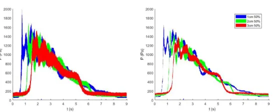
Figure 2. Particle size pressure bounds comparison.
As shown in the plots in Figure 2, the pressure bounds shift to the right as the particle size becomes larger. The left-most pressure bound using 0.01 m particles matched the experimental results with enough accuracy that smaller particles were not tested. Therefore, a particle size of 0.01 m was selected for both accuracy and acceptable run times.
Next, the measurement field size and location were adjusted. A particle size of 0.03 m was used for these comparisons to reduce the computational runtime. For changes to the measurement field size, the y-axis height of the measurement field stayed constant at a value equal to the particle size (0.03 m) because the field must be at least the size of the particles. The x-axis width value also stayed constant at 0.15 m because the experiment is considered 2-D. The z-axis length of the experiment was adjusted to see the effect on the results. Two z-axis length values were used: 0.15 m and 0.1 m.
For the location changes, only the x-axis position was varied to determine if a slight shift in location had an effect though the experiment is considered 2-D, particles are still 3-D in nature, and a shift may cause more or less particle interaction on the measurement field. The y-axis position was not adjusted because its location is based on the location of the pressure transducer in the experiment. The z-axis location also was not varied because it must stay on the end-wall of the tank. Figure 3 shows the measurement field length comparison on the left and the measurement field x-axis location comparison between centered and shifted 0.015 m on the right. These plots show the last 10 cycles of the 60 cycle simulation averaged together.
Figure 3. Measurement field size and location pressure comparison.
The values selected for each of these parameters were based on a brief parametric study of the parameter. More parameters could be adjusted, which might affect the simulation results. The following section will discuss these other parameters as well as the methodology for determining their significance.
SIGNIFICANT PARAMETER DETERMINATION
Investigated Parameters
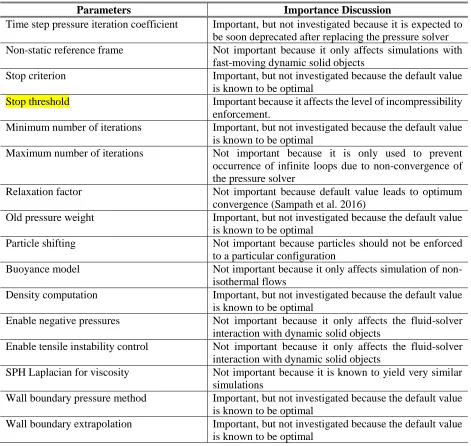
More than 30 parameters or settings are associated with a Neutrino simulation as well as parameters associated with the experiment. However, not all of these parameters have an effect on the accuracy of the simulation. Table 2 shows a list of the parameters and an initial discussion on whether the parameter was investigated to determine its significance. Highlights show parameters that were investigated.
Table 2: Parameter discussion table.
Parameters Importance Discussion
Time step pressure iteration coefficient Important, but not investigated because it is expected to be soon deprecated after replacing the pressure solver Non-static reference frame Not important because it only affects simulations with
fast-moving dynamic solid objects
Stop criterion Important, but not investigated because the default value is known to be optimal
Stop threshold Important because it affects the level of incompressibility enforcement.
Minimum number of iterations Important, but not investigated because the default value is known to be optimal
Maximum number of iterations Not important because it is only used to prevent occurrence of infinite loops due to non-convergence of the pressure solver
Relaxation factor Not important because default value leads to optimum convergence (Sampath et al. 2016)
Old pressure weight Important, but not investigated because the default value is known to be optimal
Particle shifting Not important because particles should not be enforced to a particular configuration
Buoyance model Not important because it only affects simulation of non-isothermal flows
Density computation Important, but not investigated because the default value is known to be optimal
Enable negative pressures Not important because it only affects the fluid-solver interaction with dynamic solid objects
Enable tensile instability control Not important because it only affects the fluid-solver interaction with dynamic solid objects
SPH Laplacian for viscosity Not important because it is known to yield very similar simulations
Wall boundary pressure method Important, but not investigated because the default value is known to be optimal
Wall hydrostatic pressure correction Important, but not investigated because the default value is known to be optimal
Wall viscous correction Important, but not investigated because the default value is known to be optimal
Free-surface density correction Important, but not investigated because the default value is known to be optimal
Free-surface pressure correction Important, but not investigated because the default value is known to be optimal
Near-free-surface identification coefficient Important, but not investigated because it only affects simulations with free-surface correction, which is not used
Open boundary extrapolation Not important because there is currently only a single choice and would only affect simulations with open boundaries
CFL number Important, but not investigated because the default value is known to be close to optimal
Time step diffusion coefficient Not important because it only affects simulations with highly viscous flow
Clamp to multiple of Solid-Solver time step Not important because it only affects fluid-solver interaction with dynamic solid objects
Adaptive time step Important, but not investigated because the default value is known to be optimal
SPH kernel Important, but not investigated since the same methodology can used to other smoothing kernels. Particle size Important because it changes the resolution of the
simulation.
Interaction-Radius to Particle-Size Ratio Important because it changes the number of particles influencing the particle of interest.
Fluid settling uncertainty Important because it effects the fluid depth.
Fluid depth uncertainty Not important because the correct number of particles for a given fluid depth can be calculated.
Fluid properties Not important because they will match the fluid properties of the experiment.
Measurement field size Important, but not being investigated due to initial research results.
Dimension uncertainty Important, but not investigated due to very small uncertainty range.
Forcing function amplitude uncertainty Important because it effects the forcing function of the simulation.
Forcing function frequency uncertainty Important because it effects the forcing function of the simulation.
Pressure transducer location uncertainty Important because it effects the measurement field location in the simulation.
Based on Table 2, 7 of the 37 parameters were investigated to determine their significance. These seven parameters were analysed using the method described below.
RAVEN is an Idaho National Laboratory developed analysis software. It is capable of running external codes and performing analysis on the results. RAVEN has a wide range of capabilities, a few of which include reduced order models, advanced sampling methods, data post-processing, and model parameter optimization (Rabiti et al. 2017). The Neutrino and RAVEN coupling was used so that RAVEN would sample parameter values, modify the Neutrino’s input file, and run Neutrino continuously without any user need after running the RAVEN input file (Ryan and Pope 2019).
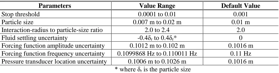
The methodology for determining the significance of parameters consisted of, first, randomly sampling across the range of possible values of a single parameter. The values were sampled from a uniform distribution across the range of values using a Monte Carlo sampler. The value range for each parameter was selected based on previous simulation investigation or the uncertainties associated with the physical experiment. The results were then analysed to determine whether the parameter caused a change in the results. If the different parameters values did not cause a change in results, then the parameter was considered insignificant. Table 3 shows the range of values for each parameter, as well as the default value that was used when other parameters were being sampled. These ranges are all considered uniform although many have other distributions.
Table 3: Investigated parameter value ranges and default value.
Parameters Value Range Default Value
Stop threshold 0.0001 to 0.01 0.001 Particle size 0.007 m to 0.02 m 0.01 m Interaction-radius to particle-size ratio 2.0 to 2.4 2.0 Fluid settling uncertainty -0.4δr to 0.4δr* 0
Forcing function amplitude uncertainty 0.1012 m to 0.102 m 0.1016 m Forcing function frequency uncertainty 0.1099868 Hz to 0.110011 Hz 0.11 Hz Pressure transducer location uncertainty 0.1006 m to 0.1026 m 0.1016 m
* where δr is the particle size
RESULTS
Validation
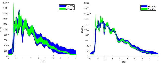
Figure 4. Pressure bounds comparison plots.
Figure 5: Pressure bounds simulation error plots.
The above plots show that both the 90% and 50% simulation pressure bounds mostly fall within the experimental bound. A few exceptions do occur in the low-pressure areas at the very beginning of the cycle (~40% difference) and the very end of the cycle (~40% difference); however, these low-pressure differences are typically insignificant for applications. The peak pressure tends to have a short but high initial peak variation (~75% difference) compared to the experiment. Overall, the simulation results match well with the experimental results for the majority of the time. However, refinement of parameters could possible increase the accuracy of the simulation.
Figure 6. Impulse pressure comparison plots.
The absolute percentage difference plot shows that the pressure impulse of the simulation is within 10% of all four experimental runs. However, for two of the runs, the simulation is within 5% of the experiment. This shows that the simulation pressure impulse matches the experimental very well.
Significant Parameters
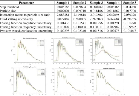
The parameters and their range of values identified above were sampled five times using RAVEN. The pressure results for all five runs were compared to determine whether the parameter is significant. To reduce the computational runtime, 30 rather than 60 cycles were simulated. Table 4 shows the five sampled values for each parameter and Figure 7 shows the average pressure plot comparison for the different parameters.
Table 4. Sampled values for each parameter.
Parameter Sample 1 Sample 2 Sample 3 Sample 4 Sample 5
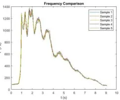
Figure 7. Average pressure comparison plots for each investigated parameter.
Based on the plots above, all seven parameters influence the simulation results. However, some of these parameters seem to be more important based on the amount of fluctuation that occurred between the results. For example, the particle size, interaction-radius to particle-size ratio, and fluid settling plots showed greater fluctuation than the stop threshold, amplitude, frequency, and pressure transducer location plots. This indicates that more research is needed to quantify the significance of each parameter.
CONCLUSION
A large-scale oscillating tank experiment was conducted and then used to validate the SPH code Neutrino, as well as determine parameters that affect the simulation results. The 90% and 50% end-wall pressure bounds were compared, as was the pressure impulse. The simulation bounds fell mostly within the experimental bounds, with exceptions at the beginning of the cycle (~40% difference), at peak pressure (~75% difference), and at the end of the cycle (~40% difference). The simulation pressure impulse matched the experiments well and was within 10%. Additionally, seven parameters were identified and investigated to determine their significance. All seven parameters were identified as significant. However, the particle size, interaction-radius to particle-size ratio, and fluid settling seem to have a greater effect due to larger fluctuation in their results.
The next step is to quantify the significance of each parameter. Once this is done, those parameters that have the greatest effect on the simulation results can be optimized. The optimization goal would be to increase the accuracy of the simulation results while still accounting for the computational runtime of the simulation. This optimization will also depend on the scenario and a valid parameter range vs result criteria needs to be established.
REFERENCES
Rabiti, C., Alfonsi, A., Cogliati, J. Mandelli, D., Kinoshita, R., Sen, S., Wang, C., Talbot, P. W., Maljovec, D. P., and Chen, J. (2017). “RAVEN User Manual,” Idaho National Laboratory, Idaho Falls, ID, INL/EXT-15-34123.
Ryan, E. D., and Pope, C. L. (2019). “Coupling of the Smoothed Particle Hydrodynamic Code Neutrino and the Risk Analysis Virtual Environment for Particle Spacing Optimization,” Submitted for publication.