TOP: A Framework for Enabling Algorithmic
Optimizations for Distance-Related Problems
Yufei Ding
North Carolina State UniversityXipeng Shen
North Carolina State UniversityMadanlal Musuvathi
Microsoft Research [email protected]Todd Mytkowicz
Microsoft Research [email protected]Abstract
This paper introduces an abstraction to enable unified treatment to distance-related problems. It offers the first set of principled under-standing to automatic algorithmic optimizations to such problems. It describes TOP, the first software framework that is able to auto-matically produce optimized algorithms either matching or outper-forming manually designed algorithms for solving distance-related problems.
1.
Introduction
A class of important problems involve certain kinds of distance calculations. They appear in various domains, including machine learning (e.g., KMeans, KNN), graphics (e.g., shortest path), im-age processing (e.g., 3D construction), scientific simulation (e.g., N-body simulation), and so on. Due to the different natures of the various problems, their distance calculations differ in many aspects, such as their definitions, patterns, constraints, purposes, and con-texts of the distance calculations. None the less, calculation of the distances among a large number of points is typically the perfor-mance bottleneck in solving these problems.
Researchers in those domains have devoted decades of efforts to create some clever algorithms to optimize the distance calculations. These efforts have beenproblem-specific. The resulting algorithm works for one problem but not others, while coming up with such algorithms usually take the domain experts lots of deep thinking, theoretical analysis, and empirical measurements. It is evidenced by the large number of papers published in the premium venues in those domains; each of them describes just one particular design of such algorithms. For instance, in the recent 10 years of top machine learning conferences, there are more than 20 papers on developing algorithms to optimize distance calculations for KMeans (e.g., [5, 10, 10, 16, 25–27]).
The objective of this work is to replace the need for such man-ual efforts with an automatic framework. We presentTriangular OPtimizer(TOP), a framework that enables automatic algorithmic optimization for various distance-based problems. With TOP, users only need to use a set of API to specify the distance problem; TOP can then automatically create an optimized algorithm for minimiz-ing the distance calculations in solvminimiz-ing the problem. TOP is ap-plicable to all problems involving distance-based calculations that meets the Triangular Inequality condition (explained later), regard-less of the domains, definition of distances, distance calculation patterns, usage of the distances, and so on. Its result matches or outperforms the algorithms manually designed by the domain ex-perts. With TOP, decades of manual efforts by the domain experts
could have been saved; it makes it much easier to create optimized algorithms to solve new distance-based problems.
The key insight underlying TOP is that all previous algorith-mic inventions for optimizing distance calculations in the various domains are essentially just variations of the usage of triangular in-equality to avoid unnecessary distance calculations. Accordingly, we propose a simple abstraction to formalize various distance-related calculations in a unified manner. The abstraction allows a systematic examination of all kinds of scenarios related with dis-tance computations, which in turn, leads to a spectrum of algo-rithmic optimizations along with some automatic mechanisms for selecting the best optimizations based on certain properties of the problem. We turn all these findings into a runtime library, the in-vocations of which in a program would automatically enable effec-tive avoidance of unnecessary distance calculations for an arbitrary distance-related problem (that meets the triangular inequality con-dition).
Along with the library, we equip TOP with a set of API and a compilation module. Through the API, programmers can easily specify the distance problem, based on which, the compiler mod-ule derives important properties of the problem, and inserts neces-sary calls to the runtime library such that at runtime, unnecesneces-sary distance calculations can be effectively detected and avoided.
Our experiments show that TOP is able to produce algorithms that match or beat the algorithms that have been designed by do-main experts. It is able to generate new algorithms for problems on which no prior work has applied triangular inequality optimizations and achieves 237X speedups.
Overall, this work makes the following major contributions:
• Abstraction:It offers an abstraction that unifies various distance-related problems to enable the first systematic study over them as a single class.
• Algorithmic Optimizations:It develops the first set of princi-pled analysis on how triangular inequality should be applied to a spectrum of distance-related problems, presents seven crys-talized principles, reduces the optimization design into two key questions (landmark selection and comparison ordering), and reveals a strand of insights in effective design of distance-related optimizations.
• TOP Framework:It builds the first software framework that is able to automatically apply algorithmic optimizations on the fly for distance-related problems.
q
c
1c’
1c
2c’
2(a) KMeans
(b) P2P
q
t
Figure 1. Example distance problems.
of the algorithms have never been proposed for the distance-related problems by domain experts.
2.
Examples for Intuition
To help convey the intuition behind TOP for optimizing distance calculations, we first describe two example problems that involve distance calculations and point out some unnecessary distance cal-culations in them.
KMeans is a popular clustering technique. It tries to group some points into K clusters. It runs iteratively. It starts with K initial centers. In each iteration, it labels every point with the center that is closest to it, and then uses the average location of the points in a cluster to update its center. It stops when the centers stop changing across iterations. In the default KMeans algorithm, each iteration has to compute the distances between every point and every center in order to find the center closest to every point. It is not necessary. Consider Figure 1 (a), where,c01 is the center of pointq in the previous iteration and c01 gets updated into c1 at the end of the previous iteration;c02 andc2 are the centers of another cluster in the two iterations. If we can quickly get the upper bound of the distance betweenqandc1, denoted asd(q, c1), and the lower bound ofd(q, c2), we may compare them first. If the former is smaller than the latter, we can immediately conclude thatc2is not possible to be the new center forxand avoid computingd(q, c2). That condition often holds as only a few points actually switch their clusters in most iterations of KMeans. The lower bound and upper bound can be more efficiently obtained than the exact distances. For instance, the upper bound of d(q, c1) can be obtained through triangular inequality ond(q, c01)andd(c1, c01), two already known distances; we will elaborate on this point in Section 4.
P2P is a second example. It is a graphic problem that tries to find the shortest path between two points in a directed graph. During the search for the shortest path among all paths between the two points, one can avoid a path if the lower bound of its length is greater than the length of the shortest path encountered so far.
3.
Unifying Abstraction
Although both involve some kind of distance calculations, the two examples described in the previous section differ in many aspects, including their domains (machine learning versus graph process-ing), natures of problem (iteratively putting points into groups ver-sus finding a path in a graph), ways distances are calculated, and purposes and constraints of distance calculations. It is hence not a large surprise that even though both problems involve unneces-sary distance calculations, no research has tried to find commonal-ities in the two problems and provide a general solution for them or other distance-related problems. Our survey finds many papers that have been published on proposing new algorithmic designs for helping each of the two problems avoid unnecessary distance cal-culations ([5, 7] for KMeans, [11, 15] for shorestPath). Similarly,
we have seen such problem-specific manual efforts in many other distance-related problems, even for some problems residing in the same domain (e.g., KNNjoin [23, 30] and KNN [14, 28]).
Despite the differences among these problems, they are all re-lated with distance calculations. A key view motivating this study is that if we can have an abstraction to which such distance-related problems can all map, we may be able to derive an automatic approach to automatically creating optimized algorithms for such problems through analyses and manipulations at that abstraction level.
Abstraction In this work, we instroduce the notion of abstract distance-related problem. It is defined as follows:
Anabstract distance-related problemis an abstract form of the problems that aim at finding some kind of relations between two sets of points, a query set and a target set; the relations are about a certain type of distances defined between the two sets of points under a certain set of constraints. We denote such a problem with a five-element tuple(Q, T, D, C, R). We explain the five elements as follows:
• Q: the query set of points. It may contain one or more points in a space of a certain dimension. It is the central entity of the relations of interest.
• T: the target set of points. It is the other party of the relations of interest.
• D: a type of distance between points.
• C: constraints related with the problem. They can be about the connectivity between Q and T, available memory in the system, or some other conditions. A special condition is whether the distance problem of interest involves many iterations of update on Q or T. If so, we call the problem an iterative distance problem.
• R: the relation of interest between Q and T. It is about the distances between those points, such as the lower bound of the distance, the closest targets to a query point, and so on.
Mappings from the Concrete The abstraction unifies various distance-related problems into a single form, making automatic al-gorithmic optimizations possible. Table 1 presents how six impor-tant distance-related problems in various domains can be mapped to the abstraction form. Each of the six problems has been ex-tensively studied in its specific domain, but they have never been treated together in a unified manner. We next explain them and the mapping briefly.
KNN is a problem that tries to find the K target points that are closest to a query point. The first row in Table 1 shows how it maps to our abstract distance-related problem. As shown in the “instantiation” part of the table, we use “x” for a single point (the query), and “S” for a point set (the target). The distance could be Euclidean or other distances, the constraint is that the memory cost should be within a given budget, and the relation of interest is to find K points from S that are closest to x. KNNjoin is similar to KNN except that its Q is a set of query points.
We have described KMeans in the previous section. It maps to our abstraction well. The set of points to cluster is Q, the center set in each iteration is T (the superscript inSt in Table 1 stands for iterative update of centers), its constraints include the iterative property besides the memory limit, and the relation of interest is the closest target for a query point.
ICP is a technique for mapping the pixels in a query image with the pixels in a target image. It is an iterative process. In each iteration, it maps each pixel in a query image with a pixel in the target image that is the most similar to the query pixel, and then transforms the query image in a certain way.
Table 1. Six Important Distance-Related Problems
Problem Domain Description Instantiation
KNN Data Mining Finding the K nearest neighbors of a query point
Q={x}, T=S, D*: Euclidean, C: mem<M, R: K points in S closest to x
KNNjoin Data Mining Finding the K nearest neighbors of each query point
Q=S1, T=S2, D*: Euclidean, C: mem<M, R: K points in T closest to each point in Q
KMeans Data Mining Clustering query points into K groups Q=S1, T=St, D*: Euclidean, C: mem<M & repeated invocations, R: the point in T that is closest to each point in Q
ICP Image Processing Matching two images Q=S1t, T=S2, D*: Euclidean, C: mem<M & repeated invocations, R: the point in T that is closest to each point in Q
P2P Graphics Finding the shortest path between two points on a directed graph
Q=S1, T=S2, D: path length, C: mem<M & graph connectivity, R: lower bound of the distance between query and target
Nbody Physics Simulate movements of particles caused by their interactions
Q=St, T=St, D: Euclidean, C: mem<M & repeated invocations, R:
set of points in T that are no farther thanrfrom a query point S,S1,S2are all sets of points, which may be identical or different; superscripttmeans that the set could get dynamically updated;xis one point; D* can be defined as other types
of distance;ris a constant give beforehand.
other in T) in a directed graph. Q and T are two sets of points on that graph, the graph connectivity is a special kind of constraint for it, the relation of interest is the lower bound of the path length between two points.
Many algorithms have been manually designed specifically for each of the five problems for avoiding unnecessary computations: KNN [8, 14, 19, 28], KNNjoin [4, 9, 23, 30, 32], KMeans [5, 7, 16, 25], ICP [12], P2P [11, 15].
Nbody is a technique for simulating the movement of many particles. It has many variations. The one used in this study is as follows. In each time step, it computes the forces imposed on a particle by all particles located within a certain range of the query point, and then updates the position of the particles accordingly. Its Q and T are the same, the set of particles, which gets updated in each iteration.
4.
Algorithmic Optimizations
With the abstraction offering a unified representation of the vari-ous distance-related problems, it becomes possible to extract the essence of the various manually designed optimizations to those problems, and reason about the principled ways for optimizing distance-related problems.
An important insight from this work is that all the previously proposed solutions are essentially just certain capitalization of tri-angular inequality in the context of the specific problem. In this sec-tion, we first give a formal presentation of triangular inequality— the fundamental vehicle for all the optimizations, and then discuss some basic conditions under which triangular inequality could help avoid unnecessary distance calculations for distance-related prob-lems. After that, we present seven principles we attain for effective capitalization of triangular inequality, which serve as the founda-tion for TOP, our automatic algorithmic optimizafounda-tion framework.
4.1 Triangular Inequality (TI): Concepts and Implications
We give the formal definition of TI as follows:
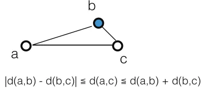
Definition 1. Leta, b, crepresent three points andd(a, b) repre-sent the distance betweenaandb;triangular inequality (TI)states thatd(a, c)≤d(a, b) +d(b, c).
Although TI does not hold for all kinds of distances, it holds for many common ones (e.g., Euclidean distance). It provides an easy way to compute both the lower bound and upper bound of the distance between two points as follows. Figure 2 offers the illustration.
|d(a, b)−d(b, c)| ≤d(a, c)≤d(a, b) +d(b, c) (1) Formula 1 offers the fundamental connection between TI and distance-related problems. Intuitively, if the lower or upper bound of the distance between two points could be used in place of their
c
a
b
|d(a,b) - d(b,c)| d(a,c) d(a,b) + d(b,c)
Figure 2. Illustration of distance bounds obtained from Triangular Inequality withbserving as alandmark.
exact distance in solving a distance-related problem, the bounds provided by Formula 1 may save the calculation of their exact distance.
But how the saving could help may not be immediately clear. As the formula shows, to get either the upper or lower bound of the distance between two points “a” and “c” in order to save the calculation of the distanced(a, c), we need two distancesd(a, b) andd(b, c). So at the first glance, there seems to be no benefits but extra cost to use the bounds. However, when we consider the context of distance-related problems, the benefits become easy to see. It relates with the concepts oflandmarkanddistance reuses that we introduce next.
Landmarks and Distance Reuses Recall that in the distance-related problem this paper defines earlier, there are two sets of points, Q and T. Suppose that the objective is to find out the upper bounds of the Euclidean distances between every point in Q and every point in T. We compare two methods. The first directly computes all the distances between the two point sets; there would beO(|Q| ∗ |T|)distances to compute. The second picks a point
x(e.g., randomly selected from Q or T), computes the distances betweenxand every point in Q and T, and then applies TI to obtain the upper bounds:d(q, t) ≤ d(q, x) +d(t, x). The number of distance computations would beO(|Q|+|T|), much smaller than in the first method when|Q|and|T|are non-trivial. We callxan intermediate point or alandmark. Using more than one landmark can help tighten the obtained bounds (to be elaborated in the next section.)
Besides spatial reuse, temporal reuse can also help exploit TI for distance-related problems. As mentioned in Section 3, some distance-related problems involve iterative update to either Q or T. It is possible to use the counterpart (q0) of a point in the previous iteration as the landmark for that point (q) in the current iteration. If the distance betweenq0and a target pointt,d(q0, t), and the move-ment of the point between the two iterations,d(q0, q), are known (or properly estimated), the bounds ofd(q, t)can be computed with TI directly; no extra distance calculations would be needed. Such distance reuses across iterations are calledtemporal reuses.
4.2 Principles for Optimization Designs
With landmarks and distance reuses, one can better understand the underlying reasons for TI to be able to help with distance-related problems. But to tap into the full potential of TI, it is essential to design the optimization to fit the given problem. Given that distance-related problems may vary in every component listed in Section 3, there is no single design that fits all. This section presents a set of design principles obtained throughout our research.
Applicability First of all, we list the basic conditions a distance-related problem should meet such that TI optimizations can apply:
•Problem Condition The solution of the distance-related prob-lem must involve some kinds of comparisons of distances among points.
•Distance ConditionThe definition of the distance involved in the comparisons must obey triangular inequality.
The Problem Condition comes from the inequality nature of TI, while the Distance Condition is necessary for TI to hold. Many distance-related problems, including all the example problems dis-cussed in Section 3, meet the conditions.
Design Objective and Dimensions There are two primary con-siderations when designing a TI optimization: optimization quality and cost. The quality is about how much computation the optimiza-tion can help avoid. It is determined by both the tightness of the distance bounds offered by TI (i.e., how close the bounds are to the exact distance) and the way the bounds are used in solving the distance-related problem. The cost is mainly about the space and time overhead introduced by the TI optimizations. TI optimizations usually require some computations and auxiliary space to work. The objective of TI optimization design is to maximize the quality while minimizing the time overhead and confining the space cost to an acceptable level (e.g., below a memory budget).
One of the most important findings in this work is that al-though the best design of TI optimizations is different for differ-ent distance-related problems, a systematic approach is possible to be developed to automatically determine the appropriate design for a given problem. Moreover, the many aspects in the design of TI optimizations can be crystallized into two dimensions: how land-marks are defined and how they are used in distance comparisons. We next explain each of the two dimensions, along with seven prin-ciples for design of TI optimizations, which are the foundation of our framework TOP.
4.2.1 First Dimension: Landmark Definition
Definition of landmarks determines the tightness of the computed distance bounds, as well as the cost of TI optimizations. We first explain some principles for effective definitions of landmarks, and then provide the whole taxonomy of definitions applicable to each category of distance-related problems.
Principle I: A good landmark for a pair of points should be close to either of the two points. That would help make the computed bounds close to the exact distance. We prove it as follows. Appar-ently, the closer lower bound and upper bound are to each other,
the tighter the bounds are. According to the definition of TI, for two pointsaandband a landmarkc, the upper bound of the dis-tanced(a, b)through TI isd(a, c) +d(b, c), while the lower bound is|d(a, c)−d(b, c)|. Their difference is2∗min(d(a, c), d(b, c)). Therefore, the closer the landmarkcis to eitheraorb, the tigher the bounds are.
Principle II: Having more than one landmark can help TI tighten bounds, if the closestLandmark information is given. ClosestLand-markinformation is about which landmark is closest to each point of interest. This principle directly follows Principle I: More land-marks, more choices, and the closestLandmark information allows TI to operate on the landmark that produces the tightest bound among all landmarks. In some cases, such information is easy to obtain and free to get, but in some other cases, it requires some computations to obtain, which could add extra cost to TI optimiza-tions. Priniple IV will elaborate on this point.
Principle III: A landmark hierarchy can help strike a good trade-off between cost and quality. Principle II says that more landmarks could help tighten bounds, but they could also increase the time and space overhead. A landmark hierarchy help address the dilemma by having more than one levels of landmarks. The bottom level has a relatively larger number of landmarks while a higher level has fewer; each landmark at a higher level represents a group of lower-level landmarks. Use of the fine-grained landmarks at the bottom level may help obtain a tight bound in some critical situation, while use of the coarse-grained landmarks at the higher levels in other situations may help reduce the space and time overhead.
Figure 3 exemplifies the benefits of a landmark hierarchy. What it shows is a small step in KMeans clustering that tries to find the center closest to a query pointq. Centers get updated in each iter-ation of KMeans. In Figure 3, we use a broken-line circle to rep-resent the location of a center in the previous iteration—which, we call theghostof the center. For instance,C10 is the ghost ofC1 in Figure 3. A possible landmark hierarchy is to use the ghosts of all centers as the low-level landmarks, and treat a group of low-level landmarks that are nearby as a high-level landmark. For instance, the broken-line oval at the top of Figure 3,G02, is a high-level land-mark corresponding to the two low-level landland-marks it contains. The usage of the two levels of landmarks is as follows. The low-level landmarkC10 is used to compute the upper bound of the distance betweenqandC1, the new position of the center that was closest toq in the previous iteration; the bound isU pBound(q, C1) =
d(q, C10) +d(C 0
1, C1). A high-level landmark is used to compute the lower bound of the distance betweenqand the group of centers corresponding to the landmark; the bound,LowBound(q, Gi), is computed as the difference betweenLowBound(q, G0i)and the maximal distance that the centers inG0ihave moved since the previ-ous iteration. IfU pBound(q, C1)< LowBound(q, Gi), no cen-ter inGiis impossible to be the center closest toq, and hence, no need to compute the distances betweenqand those centers. This example uses the low-level landmarks to ensure the tightness of
U pBound(q, C1)because it is used in the comparisons with all lower bounds. It uses the high-level landmarks for lower bounds calculation to reduce the space and time overhead: Fewer lower boundsLowBound(q, G0i)need to be recorded than using low-level landmarks for lower bounds computations, and also, fewer lower bounds need to be updated across iterations. The example demonstrates the potential benefits of having a landmark hierarchy.
q c1 c’
1
: query point
: cluster center in this iteration : cluster center in previous iteration
: group of centers in this iteration : group of centers in
previous iteration
G’2
G2
G’3
G3
Figure 3. Example of the use of landmark hierarchy in a step of KMeans.
iterative?
Q=T?
updated set
1L1M 1L2M 2L1M 2L2M
Tset
Tghost Tghost2L
Tset
Qghost Qghost2L
No Yes
Yes No
T & Q
Q T
TQghost2M
TQghost2L2M Tset+Tghost Tset+Qghost
TQghost2M
TQghost2L2M
C1 C2 C3 C4 C5
Tset+Tghost2L Tset+Qghost2L
Figure 4. Taxonomy of landmark definitions in each category of distance-related problems.
in the previous iteration. These distances can be useful in the com-putation of distance bounds in the current iteration (as illustrated in Figure 3.) Second, the ClosestLandmark information comes for free: The ghost of a point is usually the landmark close if not closest to that point when points move slowly across iterations.
Principle V: For non-iterative problems or the first iteration of an iterative problem, using some landmarks to leverage spatial reuse is often beneficial. One method is to cluster point in Q or T to create such landmarks. An alternative is to randomly select some points in Q or T as the landmarks. Although it can create the landmarks faster than clustering, the random method needs to pay the cost to find out the ClosestLandmark information. In comparison, such information comes with the clustering process in the first method. The clustering method finds landmarks better representing the points and hence is able to give tighter bounds. The clustering can be lightweight; we just run KMeans for 5 iterations and use the centers as the landmarks in our experiments.
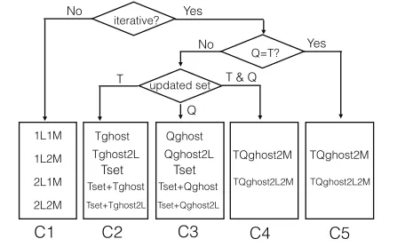
Taxonomy of Landmark Definitions Guided by those five princi-ples, we come up with a taxonomy of landmark definitions, shown in Figure 4. The graph shows the classifications of various distance-related problems into five categories based on whether the problem is iterative, whether Q equals T, and which point set gets updated across iterations (if the problem is iterative). A set of landmark def-initions suite each of the categories. We explain each of them as follows and then discuss how they are selected for a given distance-related problem.
•1L1M, 1L2M, 2L1M, 2L2M:In these definitions, “L” stands for “level”, “M” stands for “landmarks”. In all of them, there are a number of landmarks created through simple clustering as Pinciple V mentions, and these landmarks are at a low fine-grained level.
In “1L1M”, the computation of the bounds of the distance be-tween a query point and a target point is through one landmark (just like what Figure 2 shows), which shall be close to the
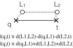
target point. In “1L2M”, the computation is through two land-marks, one shall be close to the query point, the other close to the target point, as illustarted in Figure 5. Both “1L1M” and “1L2M” leverage spatial reuses of the distances between points and landmarks and between landmarks. They differ in the num-ber of distances needed to compute. To compute the bounds between all pairs of query and target points, “1L1M” requires (m∗z+n)distances (zfor the number of landmarks): It needs to compute the distance from every query point to every land-mark, and the distance from every target to its closest landmark. On the other hand, “1L2M” requires(m+n+zq∗zt)distances (zqandztfor the numbers of landmarks closest to queries and targets respectively) since it needs the distance from each query or target to only its closest landmark, and the distances be-tween query-side landmarks and target-side landmarks. When landmarks are much fewer than queries and targets, “1L2M” needs fewer distances. However, the bounds given by “1L2M” are usually not as tight as “1L1M” gives.
The landmark definitions in “2L1M” and “2L2M” are similar to those in “1L1M” and “1L2M”, except that they also use high-level coarse-grained landmarks in addition to the low-high-level fine-grained landmarks. As explained in Principle III, the landmark hierarchy may offer better tradeoff between cost and benefits than the 1-level definitions do. The difference between “1L1M” and “1L2M” is just whether one or two landmarks are used in bounds computation. Although it is possible to have a hierarchy with more than two levels of landmarks, we have not observed much extra benefit with that increased complexity.
All these four definitions leverage spatial reuses. They suite non-iterative distance problems as well as the first iteration of iterative distance problems. The rest of definitions are specific to other iterations of iterative distance problems.
• Tghost, Qghost:These two definitions use either the ghosts of targets or queries as the landmarks, depending on which set gets updated across iterations (and hence has ghosts). As Principle IV mentions, using ghosts as landmarks for iterative problems have some special advantages: the distances (bounds) from landmarks to points are often known and the ClosestLandmark information is often available.
• Tghost2L, Qghost2L: These two definitions are similar to Tghost and Qghostexcept that a set of high-level landmarks are introduced to complement the low-level landmarks to lower the space and time overhead (just like the differences between 2L1Mand1L1Mmentioned earlier.)
• Tset:In theTsetdefinition of landmarks, points in the target set
T are used as landmarks. The bounds of the distance between
qand a target pointtis obtained by applying TI toq, t, and
L(q), where,L(q)is a target point close toq. This definition works when it is known which target is close to which query point. An example is KMeans, in which, every iteration deter-mines the center closest to each query point. Although the cen-ters may move across iterations, the movement is often small. As a result, the closest center to a query point in iteration l usu-ally remains close (if not closest) to that query point in itera-tion l+1. This definiitera-tion is not applicable to non-iterative prob-lems because the CloseLandmark information is not available in those problems. Usage of this definition for TI requires compu-tation ofd(q, L(q))andd(t, L(q)); there are|Q|computations ofd(q, L(q)), and|T| ∗ |T|computations ofd(t, L(q)). When |T| <<|Q|, the amount is still much less than the pair-wise distances between Q and T.
q
t
L
1L
2d(q,t) d(L1,L2)-d(q,L1)-d(L2,t) d(q,t) d(q,L1)+d(L1,L2)+d(L2,t)
Figure 5. Illustration of how two landmarks can be used for com-puting lower and upper bounds of distances.
Tghost or Tghost2L are then used for attaining tighter bounds for that pair. Such a combination could be beneficial because checks with Tset are faster to do while the bounds from Tset are not very tight. The combination gets the best of both worlds. Tghost2L is preferred over Tghost if space is an issue. •TQghost2M, TQghost2L2M: TQghost2Mis similar toTQghost
except that to compute the bounds of a distance, it uses two landmarks: One is the ghost of the query, the other is the ghost of the target. The usage of this landmark definition needs to have the distances or their bounds between every pairs of query and target recorded in each iteration, which could incur large space and time overhead. TQghost2L2M includes high-level landmarks to lower the space and time cost (in a vein similar to2L1Mversus1L1Mmentioned earlier).
These two definitions apply only when Q=T or Q and T both get update across iterations since in other cases, either the query or the target has no ghost. On the other hand, the definitions that apply to the other cases do not apply to these two cases because those definitions all assume that either the target or the query remains unchanged across iterations.
Selecting Landmark Definitions As Figure 4 shows, multiple landmark definitions may apply to a distance-related problem, and one definition can have many possible configurations (e.g., number of landmarks).
For a given distance-related problem, the suitable landmark definition should have an acceptable space cost and at the same time minimize the time for solving the problem. Space cost includes the space for storing landmarks and distances or bounds from points to landmarks. It is mainly determined by the size of the problem and the number of landmarks the definition uses. Given such information, the cost can be computed analytically; during our explanation of the taxonomy of definitions, we have already mentioned the space cost required by them.
Execution time is more complicated. The TI optimization helps avoid some distance calculations between queries and targets, but also introduces time overhead, including the time for computing distance bounds between queries and targets, distances (or bounds) from landmarks to queries or targets, and extra comparisons among bounds and distances for avoiding distance calculations. The ben-efits and costs depend on the size of the problem, the number of landmarks, but also the locations or distributions of the queries and targets. It is more difficult to compute the time cost and benefit analytically. One option is to use runtime sampling to model the distributions of the points, based on which, it infers the amount of distance computations each definition may avoid and estimates the time benefits and cost accordingly. Due to its complexity, we leave this option for future study. In this work, we instead use a sequence of rules obtained empirically for definition selection. These rules are not intended for optimal selections, but offer a simple way to make good selections in practice.
The rules together form a selection algorithm. For lack of space, we omit a thorough discussion to the Appendix, where the type and number of landmarks are decided.
4.2.2 Second Dimension: Comparison Order
Besides landmark definition, another important dimension for TI to work effectively is how the bounds TI produces are used, particu-larly, the order of using the bounds for distance comparison. For example, one wants to find a target closest to a queryq. Letdmin be the shortest distance currently found betweenqand targets. For a targett, before computingd(q, t), one can first check whether the lower bound ofd(q, t)(obtained through TI) is larger thandmin and skip computingd(q, t)if so. In this example, the comparison order refers to the order in which the targets are checked. If the order is an ascending order of the lower bounds ofd(q, t)among allt, the check can stop immediately when it encounters one target whose lower bound is greater thandmin: All the remaining targets must have lower bounds greater thandminas well because of the ascending comparison order.
Our analysis gives the following two principles regarding com-parison order. They help not just save distance comcom-parisons, but avoid computing unnecessary lower bounds at the first place. The principles apply to a set of targets that share a landmark—that is, the landmark used would be the same if one wants to apply TI to compute the distance bounds between a query point and each of the targets. An example is whenT setis used as landmarks for KMeans. For a given query, all targets share the same landmark (i.e., the landmark closest to the query).
Principle VI: When the objective of distance comparisons is to find the targets closest to the query, the comparison order should be the ascending order of the distances from the targets to the landmark if the landmark is closer to the query than to the targets, and should be the descending order of the distances otherwise.
Principle VII: When the objective of distance comparison is to find the target farthest from the query, the comprison order should be the descending order of the distances from the targets to the landmark.
Principle VI ensures that the order is the same as the ascending order of the lower bound of the distances from target to query. To see it, one just need to notice that the lower bound equals
d(l, t)−d(l, q)if the landmark is closer to the query, and equals
d(l, q)−d(l, t)otherwise (wherelfor landmark,tfor target, and
qfor query). Principle VII ensures that the order is the same as the descending order of the upper bound of distances from target to query. It is because the upper bound equalsd(l, t) +d(l, q)no matter wherelis.
When the two principles are used for distance comparison, many targets that are impossible to be the closest or farthest could be skipped from consideration. If a target is skipped from consid-eration, its distance from the query need not get computed, and at the same time, the computation of the lower bound of the distance from it to the query can be also skipped since the two principles use the distance from targets to landmarks rather than the lower bounds for ordering.
5.
TOP Framework
To translate the abstraction and optimizations into applicable tools, we design a software framework named TOP (which stands for triangular optimization). TOP consists of three components: a set of API that users can use to formally define a particular distance-related problem, a runtime library that implements the principles and rules for creating optimized algorithms to fit the user-defined distance problem, and a compiler module that helps the runtime obtain necessary information.
5.1 API
module and runtime. The key point of these API is to express the algorithm in terms of the five components we defined before: query set Q, target set T, constraints C, distance definition D, and inter-point relations of interest R.
5.2 Runtime Library
The runtime library consists of three parts. The first part is for se-lecting and configuring landmark definitions. At its core is a func-tionpickLandmarkDefthat implements the algorithm for selecting and configuring landmark definitions as what was shown in Fig-ure 9 in Section 4. Runtime invocation of this function will de-termine the landmark definition suiting the particular problem in-stance. The second part is for materializing the TI optimizations. It contains a set of functions that implement the TI-based optimiza-tions for the various kinds of relaoptimiza-tions listed at the bottom part of the TOP API. For each of the relation, a number of versions are created with each as an optimized algorithm based on one type of landmark definition. Each of them records necessary bounds or dis-tances for the TI to work, and applies TI by drawing on the land-marks to avoid as many distance computations as possible. These first two parts of the TOP runtime library form the low-level API of TOP. The third part of the library is the implementations of the TOP API in Figure 10, which we call the high-level API. The im-plementation of each high-level API at the bottom section of Fig-ure 10 contains some condition checks such that it invokes the cor-rect TI-optimized algorithm by calling the right low-level API func-tion contained in the second part of the library.
For instance, the second part of the library contains 15 func-tions that each implements a TI-based algorithm to find the clos-est targets for a query point. They all try to use TI to clos-estimate the lower bound of the distance between a query point and a tar-get and avoid computing their distances if the lower bound is larger than the current minimum distance. They differ in what land-marks are used for getting the lower bounds, and in the opera-tions related with the maintainence of the landmarks. Invocation of TOP findClosestTargets selects one of them based on the category of the current problem and the definition of the landmarks that has been selected. For the KMeans example shown in Figure 11, one of the versions corresponding to the four definitions in category 2 will be selected depending on the result of the function pickLand-markDef.
The versions in the library subsume existing manually designed problem-specific algorithms that leverage TI. They often go beyond them thanks to the taxonomy we obtain through this systematic treatment to distance-based problems. Section 6 will show that the outcome from TOP optimizations either match or beat prior manually designed algorithms.
5.3 Compiler Module
The main functionalities of the compiler module are two-fold. First, it inserts invocations of some low-level API calls (e.g., pickLand-markDef) into the original program. Second, it analyzes the code to determine whether the problem is iterative and which data set gets updated across iterations. It passes these information to the runtime library by inserting several low-level API calls before the invocation ofpickLandmarkDef. In the similar way, it helps inform the TOP runtime library other necessary information (e.g., size and dimensionality of data sets) that are collected at runtime. The im-plementation of the compiler is based on LLVM [20].
6.
Evaluation
TOP is an powerful automatic tool that can be applied to various of distance related problems. To demonstrate its efficacy, we ran it on six algorithms and compared their performance with the manually optimized versions developed in previous paper. Both the generated algorithm from TOP and manually optimized versions are in C++.
Table 2. Averaged Ratio of Eliminated Compuations
Problem TOP Previous Works
KNN 92.98% 92.98%
KNNjoin 95.56% 95.55%
KMeans 92.84% 96.83%
ICP 99.63% 97.53%
P2P 93.22% 93.22%
Nbody 99.44% 0
For each problem, we tested both versions on the same set of inputs, most of which are coming from those used in previous paper. As each pair of algorithms follow the same semantics and would generate the same results when same inputs and running configurations are used, the quality of results is not a problem here. Instead, we would focus on the performance of algorithms.
6.1 Efficiency
Triangle inequality optimization, as we discussed, is to eliminate redundant computations in the program. For some of them, like KNN, kmeans, it is to remove unnecessary distance computations through high quality lower bound and upper bound computations. While for others, like P2P, it is to accelerate the search process with good estimation of the distance(path) between two points. In our experiments, we report both the left computations, and average running times for both set of algorithms. The concept of computa-tions can be different for different algorithms, for example, for Knn, Kmeans, KNN, ICP, Nbody, it is the number of distance computa-tions; and for P2P, it is the number of visited vertices. Measurement of such computations is machine-independent and a good measure of algorithm performance, especially when these computations are the most time consuming part in the original algorithm. We also re-port the average running times of both set of algorithms to provide a better understanding of practical performance when the algorithms are ran on a specific machine, where the amount of computation and memory sources are limited.
6.1.1 Pruned Computations
Number of Computations (Previous Works)
0 106
1013
Number of Computations (TOP)
106 1013
Knn Knnjoin Kmeans ICP Nbody P2P Reference line
Figure 6. Number of pruned computations
Speedup of Previous Works (Runtime)
0 1 102
104 Speedup of TOP (Runtime) 1
102 104
Knn Knnjoin Kmeans ICP Nbody P2P Reference line
Figure 7. Speedup of averaged running time over default imple-mentations
previous iteration, and as a consequence, limits its applicability. For inputs with larger k — the size of the target set, such overhead can be much larger than the original input size and can not fit in the memory. Points on the y-axis of figure 6 is a result of such case. On the other hand, our version from TOP framework takes the memory size of the specific machine into account. And through grouping, it reduces the space overhead and enhance the applicability.
6.1.2 Running times
Figure 7 shows the running times for six pairs of algorithms under the same set of inputs, which are used in figure 6. As expected, these two figures show close correlations, and five out of six algo-rithms give the same trend of performance. However, such trend gets reversed for Kmeans, where our TOP shows shorter running time for most of the inputs. With further test and analysis, we found the reason of good performance of our TOP version as follows. Due to the strong pruning of both our and the manually optimized ver-sion, most of the distance computations get pruned, and as a re-sult, distance computation is no longer the dominate cost of the op-timized version. In comparison, updating these historic distances, along with comparisons between the upper and lower bounds be-come an important cost. With grouping, our TOP framework re-duces such costs and improves the overall performance.
6.1.3 Elasticity
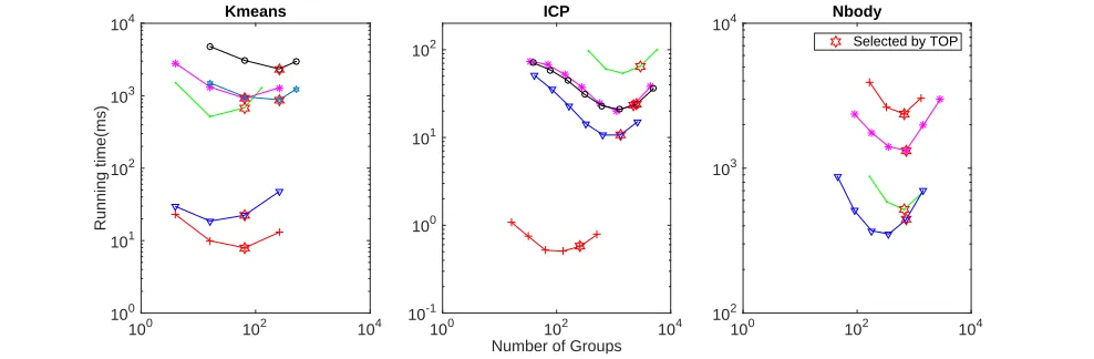
Temporal optimization provides good ways to pick up the interme-diate point set, and further, through reusing of the historic distance results, it shows great power of pruning redundant computations.
Generally speaking, the more distance information we maintained across iterations, the more redundant computations we can elim-inate. However, with more distances maintained across iterations, we need more space to store them, and more cost to update and check them. Fortunately, our grouping strategy provides a solution to strike a balance between the pruning power and the overhead. Figure 8 shows the overall running times as the function of the number of groups of the query set, and each curve in the figure stands for the performance of one special input. As expected, fig-ure 8 demonstrates that by increasing the number groups, the over-all running time first decreases, then increases when the number of groups further increases. Three iterative algorithms, ICP, Kmeans and Nbody, for which temporal optimization are applied, give the same trend of performance changes. In our TOP framework, the number of groups are decided automatically, based on the size of memory and size of the query and target set. On average, the run-ning time based on such strategy is within 13% percentage from the best performance by varying the number of groups.
We also carried out two case studies to show how different algorithmic option affect the performance. Due to the space limit, we put two of them into the Appendix.
7.
Related Work
Triangle inequality has been used for many distances related prob-lems, like the six algorithms we discussed in the paper. For lack of space, we omit a thorough discussion of all the previous works. And our discussion will focus on these six algorithms and the ver-sion we used in the paper for comparison.
K nearest neighbor (KNN) queries is an important problem in spatial databases, e.g., road networks. Many researches has focused on this problem to accelerate the search process. Generally, these existing work are based on either different kinds of tree structures [18, 21], or triangle inequality [14, 28]. In [28], Xueyi relies on the latter and compares his algorithm to the previous k-d tree and ball tree implementations, and shows better overall performance. In particular, it uses Kmeans to partition the target point set. And the distance from the query point to the target point are estimated through the landmark in each partition based on triangle inequality. Knnjoin can be regarded as a combination of the k nearest neighbor query and the join operation, and it is widely adopted by many data mining applications as a primitive operation. To compute distances among a large amount data is an important problem and has been investigated through various perspectives [23, 30, 31]. In [23], Lu suggests to partition both query and target into groups and compute bounds of distance between query and target point through landmarks they are assigned to, based on triangle inequality. As a result, instead of computing the exact distance between every pair of query and target points, bounds of distances are used as substitutions when possible.
KMeans, as a method of clustering multidimensional data, has been used in various areas, e.g. bioinformatics, astrophysics, vector quantization, and computer vision. Various prior efforts try to im-prove naive kmeans [22], both in terms of speed and cluster quality, as discussed in [1, 7, 17, 24]. Among them, Kanungo’s work [17] based on k-d tree and Elkan’s work [7] based on triangle inequality are the two main branch that focus on improving the speed. The former is good for lower dimensional data, while the later shows good performance across inputs with all dimensional data. In the paper, we use Elkan’s algorithm as the previous work for compar-ison. Elkan uses the triangle inequality to to compute one upper bound and k lower bounds per each data point. By recording and efficiently updating these bounds across iteration, it avoids calcu-lating the explicit distance between a point and a center, whenever the lower bound is larger than the upper bound, and results in sig-nificantly acceleration of kmeans.
100 102 104
Running time(ms)
100 101 102 103
104 Kmeans
Number of Groups
100 102 104
10-1 100 101 102
ICP
100 102 104
102 103
104 Nbody
Selected by TOP
Figure 8. Running times as a function of the number of groups/landmarks
mapping between two overlapping surfaces and uses the mapping to guide the transformation. One of the main drawbacks of the algorithm is its quadratic time complexityO(n2)with the number of pointsn. Various of previous work has been used to accelerate the process [12, 13] . In [12], Greenspan demonstrates how to uses triangle inequality to find the mapping between two sets of points efficiently and their results are better than previous strategy based on k-d tree and Elias methods. In their implementation, each query point uses its best mapping — closest target point from last iteration as the bridge, to estimate its distance to other query points. As the query set is fixed across iteration, the cost of computing distances among target point can be amortized.
Point to point (P2P) shortest path problem is a fundamental problem with numerous applications, e.g. providing driving direc-tions for GPS devices. Traditional way to search for the shortest path is based on Dijkstra’s algorithm [3]. Obviously it is not a ef-fective solution, later work tries to improve the efficiency by re-ducing the number vertices along the search path. Lower bounds of path between two vertices are found important and are utilized in different works to accelerate the search process [11, 15]. In [11], Andrew uses A*, combined with lower bounds computations based on triangle inequality to improve the efficiency and achieves great speedup, and this is also the one we used for comparison.
Nbody simulation [6] studies the evolution of a dynamical system of multiple particles, under the influence of physical forces. It has been used for various problems in the area of physics and astronomy. Due to the large number of particles in the system, computations of interactions between every two particles would be huge and sometimes unaffordable. Various of previous work has been done to improve its speed [2, 29]. In particular, when the force are short-ranged, it is possible to use the neighbor list, which includes all points within a certain radius to guide the simulation. Previous work to accelerate neighbor list computation process is based on cell lists [29], which is similar to tree structure used in previous algorithms. We did not find any previous work based on triangle inequality and findings here could be a good alternative solution.
8.
Conclusion
This paper presents an effort to enable automatic algorithmic opti-mizations for distance-related problems. It develops the first set of principled analysis on how triangular inequality should be applied to a spectrum of distance-related problems. The resulting frame-work TOP is able to produce algorithms that either match or beat manually designed algorithms for a list of important problems.
References
[1] D. Arthur and S. Vassilvitskii. k-means++: The advantages of careful seeding. InProceedings of the eighteenth annual ACM-SIAM sympo-sium on Discrete algorithms, pages 1027–1035. Society for Industrial and Applied Mathematics, 2007.
[2] N. Bou-Rabee. Time integrators for molecular dynamics.Entropy, 16 (1):138–162, 2013.
[3] E. W. Dijkstra. A note on two problems in connexion with graphs. volume 1, pages 269–271. Springer, 1959.
[4] H. Ding, G. Trajcevski, and P. Scheuermann. Efficient similarity join of large sets of moving object trajectories. InTemporal Representation and Reasoning, 2008. TIME’08. 15th International Symposium on, pages 79–87. IEEE, 2008.
[5] J. Drake and G. Hamerly. Accelerated k-means with adaptive distance bounds. In5th NIPS Workshop on Optimization for Machine Learning, 2012.
[6] V. Eijkhout. Introduction to High Performance Scientific Computing. Lulu. com, 2010.
[7] C. Elkan. Using the triangle inequality to accelerate k-means. In
ICML, volume 3, pages 147–153, 2003.
[8] C. Elkan. Nearest neighbor classification. University of California– San Diego, 2007.
[9] T. Emrich, F. Graf, H.-P. Kriegel, M. Schubert, and M. Thoma. Optimizing all-nearest-neighbor queries with trigonometric pruning. InScientific and Statistical Database Management, pages 501–518. Springer, 2010.
[10] A. Fahim, A. Salem, F. Torkey, and M. Ramadan. An efficient en-hanced k-means clustering algorithm.Journal of Zhejiang University SCIENCE A, 7(10):1626–1633, 2006.
[11] A. V. Goldberg and C. Harrelson. Computing the shortest path: A search meets graph theory. InProceedings of the sixteenth annual ACM-SIAM symposium on Discrete algorithms, pages 156–165. Soci-ety for Industrial and Applied Mathematics, 2005.
[12] M. Greenspan and G. Godin. A nearest neighbor method for efficient icp. In3-D Digital Imaging and Modeling, 2001. Proceedings. Third International Conference on, pages 161–168. IEEE, 2001.
[13] M. Greenspan and M. Yurick. Approximate kd tree search for efficient icp. In3-D Digital Imaging and Modeling, 2003. 3DIM 2003. Pro-ceedings. Fourth International Conference on, pages 442–448. IEEE, 2003.
[14] M. Greenspan, G. Godin, and J. Talbot. Acceleration of binning nearest neighbor methods. InVision Interface, Montreal, Canada, May 14-17, page 337–344. IEEE, 2000.
[16] G. Hamerly. Making k-means even faster. InSDM, pages 130–140. SIAM, 2010.
[17] T. Kanungo, D. M. Mount, N. S. Netanyahu, C. D. Piatko, R. Silver-man, and A. Y. Wu. An efficient k-means clustering algorithm: Anal-ysis and implementation. volume 24, pages 881–892. IEEE, 2002. [18] Y. J. Kim and J. M. Patel. Performance comparison of the {rm
R}ˆ{ast}-tree and the quadtree for knn and distance join queries. volume 22, pages 1014–1027. IEEE, 2010.
[19] J. Z. Lai, Y.-C. Liaw, and J. Liu. Fast k-nearest-neighbor search based on projection and triangular inequality. Pattern Recognition, 40(2): 351–359, 2007.
[20] C. Lattner and V. Adve. Llvm: A compilation framework for life-long program analysis & transformation. InCode Generation and Optimization, 2004. CGO 2004. International Symposium on, pages 75–86. IEEE, 2004.
[21] T. Liu, A. W. Moore, and A. G. Gray. Efficient exact k-nn and non-parametric classification in high dimensions. InAdvances in Neural Information Processing Systems, page None, 2003.
[22] S. Lloyd. Least squares quantization in pcm. volume 28, pages 129– 137. IEEE, 1982.
[23] W. Lu, Y. Shen, S. Chen, and B. C. Ooi. Efficient processing of k nearest neighbor joins using mapreduce. Proceedings of the VLDB Endowment, 5(10):1016–1027, 2012.
[24] A. W. Moore. The anchors hierarchy: Using the triangle inequality to survive high dimensional data. InProceedings of the Sixteenth conference on Uncertainty in artificial intelligence, pages 397–405. Morgan Kaufmann Publishers Inc., 2000.
[25] W. K. Ngai, B. Kao, C. K. Chui, R. Cheng, M. Chau, and K. Y. Yip. Efficient clustering of uncertain data. InData Mining, 2006. ICDM’06. Sixth International Conference on, pages 436–445. IEEE, 2006.
[26] D. Sculley. Web-scale k-means clustering. InProceedings of the 19th international conference on World wide web, pages 1177–1178. ACM, 2010.
[27] J. Wang, J. Wang, Q. Ke, G. Zeng, and S. Li. Fast approximate k-means via cluster closures. InComputer Vision and Pattern Recog-nition (CVPR), 2012 IEEE Conference on, pages 3037–3044. IEEE, 2012.
[28] X. Wang. A fast exact k-nearest neighbors algorithm for high dimen-sional search using k-means clustering and triangle inequality. In Neu-ral Networks (IJCNN), The 2011 International Joint Conference on, pages 1293–1299. IEEE, 2011.
[29] Z. Yao, J.-S. Wang, and M. Cheng. Improved o (n) neighbor list method using domain decomposition and data sorting. 2004. [30] C. Yu, B. Cui, S. Wang, and J. Su. Efficient index-based knn join
pro-cessing for high-dimensional data.Information and Software Technol-ogy, 49(4):332–344, 2007.
[31] C. Zhang, F. Li, and J. Jestes. Efficient parallel knn joins for large data in mapreduce. InProceedings of the 15th International Conference on Extending Database Technology, pages 38–49. ACM, 2012. [32] D. Zhang, C.-Y. Chan, and K.-L. Tan. Nearest group queries. In
Proceedings of the 25th International Conference on Scientific and Statistical Database Management, page 7. ACM, 2013.
A.
Appendix
A.1 Landmark SelectionBased on the rules we learn, we develop a selection algorithm as show in Figure 9. For category 1, the algorithm uses 2-level land-marks if the platform is a distributed system, and 1-level otherwise. The number of top-level landmarks in the 2-level case equals the number of computing nodes on the platform. Regarding whether TI should be applied with one or two landmarks each time, the algorithm first examines how many landmarks the space budget allows if the one-landmark scheme is used. If it is too few (less thanp(|Q|)), the one-landmark scheme is unlike to offer tight distance bounds, and the two-landmark scheme should used. Be-cause the two-landmark scheme does not require as many distances to be stored as one-landmark scheme requires, the space budget could allow more landmarks created and hence offer tighter dis-tance bounds.
For category 2, the algorithm first decide whether Tset should be used. Since Tset needs the computation of the distances between every pair of targets, it applies only when|T|is small (less than 0.01∗ |Q|). After that, the algorithm tries to decide whether Tghost or Tghost2L should be used in case that the bounds from Tset are not tight enough. One condition is whether there are enough space for Tghost. If so,d, the number of dimensions of the data space, is checked. Tghost is used only ifdis large enough (no smaller than 1000). Otherwise, Tghost2L is used. The condition ondcomes from the following reason. Tghost may avoid more distance calcu-lations than Tghost2L does because it always use low-level land-marks for bound computations. However, it adds more bound com-putations and distance checks than Tghost2L does—Tghost2L do bound computations and distance checks only once for a group of rather than every low-level landmarks. So, Tghost is better only if a distance calculation is much more costly than a bound computation or check. The cost of a distance calculation is mainly determined by the number of dimensions of the data space, hence the condi-tion. Treatment to category 3 is the same as to category 2 except that Qghost or Qghost2L rather than Tghost or Tghost2L is used.
For categories 4 and 5, the main question is whether 1-level or 2-level landmarks should be used. The conditions to check are the same as those checked for determining the number of landmark levels in category 2.
After the type of landmark definition is determined, function “configure” sets up the number of landmarks to generate. For cat-egory 1, the number of low-level landmarks is 2p
|Q| for the query set and2p|T|for the target set. Such numbers come from previous domain-specific explorations [23, 28], which each stud-ies only a specific distance-related problem, but finds the same choice of the number of landmarks that works well. If two lev-els are used, the number of landmarks at the top level equals the number of computing nodes in the distributed system. For the other categories, the number of low-level landmarks either equal to|T|or|Q|since the landmarks are just their ghosts. When the 2-level scheme is used, the number of the top-2-level landmarks equals
q
2∗p
|X| ∗ |X|/10, whereX should be replaced withT orQ
depends on which set the landmarks are created for. This formula is a combination of the considerations for the spatial and temporal reuses. Recall that for iterative problems, we exploit spatial reuse for the first iteration and temporal reuse for the future iterations. The first part of the formula,2∗p
input: query setQ, target setT, number of dimensions of the data spaced, space budgetBudget, category of the problemcat. ifcat==1then
// to use 1-level or 2-level landmarks
L=1;
ifdistributedPlatformthen L=2;
end if
// to use 1 or 2 landmarks as intermediate points
M=1;
nMax=maxLandmarks(Budget, cat, L, M,|T|,|Q|); ifnMax<p
|Q|then M=2;
end if end if
ifcat== (2k3)then
// to decide whether Tset is to be used
useTset=false;
if|T|<0.01∗ |Q|then useTset=true; end if
// to select Tghost/Qghost or Tghost2L/Qghost2L
ifcat==2then
spaceNeeds = estimateSpaceCost(Tghost, |T|, |Q|,useTset);
else
spaceNeeds = estimateSpaceCost(Qghost, |T|, |Q|,useTset);
end if L=1;
ifspaceNeeds>Budgetkd<1000then L=2;
end if end if
ifcat==(4k5)then
// to select TQghost2M or TQghost2L2M
spaceNeeds = estimateSpaceCost(TQghost2M,|T|,|Q|); L=1;
ifspaceNeeds>Budgetkd<1000then L=2;
end if end if
// to set the number of landmarks based on space budget
configure(Budget, cat, L, M,|T|,|Q|);
Figure 9. Algorithm for selecting landmark definitions.
A.2 API
We introduce a small set of API, with which, users can easily define their distance-related problem in a way that it can be analyzed and handled by the TOP compiler module and runtime. The API in our current implementation is intended to be used with C or C++ languages; it can be easily modified to work with other languages.
As Section 3 lists, there are five components of a distance-related problem: query set Q, target set T, constraints C, distance definition D, and inter-point relations of interest R. The API con-tains entries for specifying each of them, as summarized in Fig-ure 10. It includes some predefined structFig-ures for a data point and a point set. It has a cost matrix structure TOP costMat for expressing connection constraints among points (e.g., points in a graph). Let
M be a TOP costMat; ifM[i, j] >= 0, there is an edge from point i to point j with edge weight equalingM[i, j]; otherwise, no edge between them. It is symmetric if the graph is undirected. There are some other structures defined for representing sparse ma-trices or graphs, which are not shown in Figure 10. There are some APIs to faciliate users in constructing cost matrices which are
omit-Predefined structures:
TOP_point, TOP_pointSet, TOP_costMat, …
API for Constraints:
TOP_update (TOP_pointSet S, int * changedFlag, …); some facilities for cost matrix construction;
API for Distance:
TOP_defDistance (enum);
TOP_defDistance (TOP_point, TOP_point, TOP_costMat);
API for Relation:
TOP_getLowerBound (TOP_pointSet, TOP_pointSet, TOP_costMat); TOP_getUpperBound (TOP_pointSet, TOP_pointSet, TOP_costMat); TOP_findClosestTargets (int, TOP_pointSet, TOP_pointSet, TOP_costMat); TOP_findFarthestTargets (int, TOP_pointSet, TOP_pointSet, TOP_costMat); TOP_findTargetsWithin (float, TOP_pointSet, TOP_pointSet,TOP_costMat); TOP_findTargetsBeyond (float, TOP_pointSet, TOP_pointSet, TOP_costMat);
Figure 10. Core APIs defined in TOP.
/*Goal: Cluster points in S into K classes with T containing all cluster centers S: a set of query point to cluster.
T: a set of target point, that is, the cluster centers. N: a set of index of points. |N|=|S|.*/
… // declarations
TOP_defDistance(Euclidean); T = init();
changedFlag = 1; while (changedFlag){
N = TOP_findClosestTargets(1, S, T); TOP_update(T, &changedFlag, N, S); }
Figure 11. KMeans written in TOP API.
ted in Figure 10. In addition, the API for constraints contains a TOP update function, which users may implement to update a point set S. Its returned value in ”changedFlag” indicates whether the point set gets actually updated. This function helps compiler and runtime determine whether the distance problem iteratively updates a point set and which set it is. The API for distance definition in-cludes a function to specify the distance in the problem if it is one of a set of predefined distances (Euclidean etc.) that are amenable to TI. It has another function which users may implement to de-fine their own distances. It would be the users’ responsibility to ensure that the distance is amenable to TI. Automatic inference of the property could be possible, but not in the current implementa-tion of TOP yet. The final part of the API is for specifying the kind of relations of interest between query points and target points. TOP currently includes four basic relations: get the lower bound of a dis-tance, get the upper bound of a disdis-tance, find a certain number of targets that are closest or farthest to a query point, find all the tar-gets that reside within or beyond a certain distance from the query point. There are some variations of some of the API functions that are elided in Figure 10 (e.g., using a sparse cost matrix). Using the API to define a distance problem is simple. Figure 11 illustrates the usage of TOP API by showing the important part of KMeans written in the API.
A.3 Case studies:
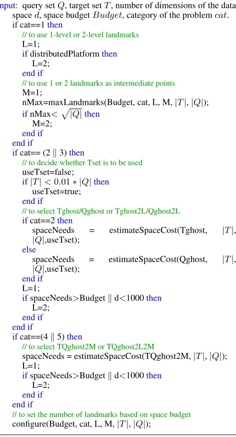
A.3.1 Spatial vs Temporal Optimization for ICP
Different input settings (ICP)
Number of Distance Computations
102 104 106 108 1010 1012
Default
Spatial Optimization Temporal Optimization
Figure 12. Averaged number of distance computations per itera-tion with spatial and temporal optimizaitera-tion
first, it reduces the starting-up cost for transitional usage of tem-poral optimization. Take Kmeans as example, the manually opti-mization version from previous paper does not optimize the first iteration, where distances from every query and target points are calculated. Its main purpose is to get a tight bound of these dis-tances and improve the pruning power of later iterations. But we find that for those far-away target points, there is no need to get such tight bounds anyways, in that, the slightly relaxed bounds, obtained from spatial optimization, would already give great prun-ing power. Second, temporal optimization is great to apply when the changes of query/target set are small across iteration, this can be easily satisfied for most iterative algorithm, especially for their later iterations. However, for the first one or several iterations, it is still common that the changes of query/target set is relative large, and as a result, the performance of temporal optimization is not as good as spatial optimization. Figure 12 shows a case study of the ICP algorithm, where both spatial and temporal optimization are used. We found that for inputs we tested, our TOP framework chooses spatial optimization for the first iteration and temporal op-timization for the later iterations. And three bars in figure 12 shows the averaged number of distances per iteration for the default, our spatial and temporal optimization. Here default refers to the naive implementation, where distance between every query and target points are computed. It shows that the spatial optimization removes over 90% percentage of distance computations, but still maintains a good quality of bounds for later temporal optimization, for which there is less than one distance computation for each query point on average.
A.3.2 Ordering inside Group for KNN
As discussed, ordering of points inside each group could be ben-eficial in that the transverse of points can be terminated earlier. In figure 13, we studied how ordering would affect the performance for KNN. We compared the averaged running time of two ver-sions on a set of inputs: first one is automatically selected version from our TOP, where points inside each group is ordering descend-ing based on its distance to the landmark; second is the one we manually implemented, for which only the maximum distance is recorded for each landmark. Figure 13 shows that by adding this ordering, the first version outperforms up to3.89Xbetter than the second version. Besides, we tried three options of k —the number of neighbors— for each input. It can be seen that speedup decreases with increasing of k. It is easy to understand, in that the possibility for a point to be one of the k nearest neighbor increases with larger k. And based on our empirical study, we find that the speedup di-minishes when k reaches the size of group.
Due to the space limit, we will not show how the dimension d of point affect the ordering here. But the conclusions are as
Input Size (n)
103 104 105
Speedup(Runtime)
1 1.5 2 2.5 3 3.5 4
k = 10 k = 40 k = 160
Figure 13. Running times as a function of the number of groups/-landmarks
the follows: speedup gained from ordering would decrease with increasingd, and such speedup would diminish when d reaches √