3029
Mixed Stochastic Input Oriented Data
Envelopment Analysis Model
Nahia Mourad, Assem Tharwat
Abstract: Data envelopment analysis (DEA) is a mathematical tool used to evaluate relative efficiency of decision-making units (DMUs). It is a bench-marking method for these units. To measure this relative efficiency, data related to a set of inputs and outputs are provided from all the DMUs under analysis, and then implemented in a suitable DEA model. Stochastic DEA allows the inputs or outputs to be stochastic random variables. In this article, we consider combination of deterministic and stochastic inputs following Normal and/or Poisson distribution. To the best of our knowledge, variables following Poisson distribution are not yet considered in these methods. We introduce the stochastic input -oriented data envelopment analysis (SIODEA) model. The random inputs, following either normal or Poisson distributions, are controlled by chance constrained. Using functional analysis techniques, the chance constrained with Poisson variables is replaced by difference of Marcum functions evaluated at points related to th e parameters of these variables. Consequently, we formulate a deterministic equivalent model with mixed random inputs. Finally, a numerical example is presented and the efficiencies of different DMUs are calculated using the obtained equivalent model to test its validity.
Keywords: Mathematical Programming, Performance, Efficiency, Decision Making, Data Envelopment Analysis, Input Oriented DEA, Stochastic Inputs, Chance Constrained
—————————— ——————————
1
INTRODUCTION
Data envelopment analysis has become a powerful tool for measuring product or organizational performance [14]. It was first introduced by Charnes and Cooper [7], in 1978. DEA, which is a non-parametric method, uses mathematical programming to analyze the performance of comparable organizations. These organizations are known by the decision-making units. Information regarding predetermined inputs and outputs are gathered from different DMUs and implemented in a suitable DEA model. Using this model, one can computes the maximum relative efficiency of each DMU under analysis. DEA method is not restricted to business and economics problems. It has a wide range of applications in different fields. This method is used to compute the efficiency in agriculture [1, 5, 20], ecological development [8], consumption and production of energy [20, 27, 28], etc. It is especially used in the studies of sustainable energy [12, 21]. More applications of DEA, in various fields, can be found in the literature. The efficiency score is the ratio of the weighted output to the weighted input [29]. This produces a DEA ratio problem. This last is transformed from fractional programming to linear programming, forming either input or output oriented model. Finally, the dual of this last formulation is generated (for more details refer to [2]). In this paper, we will consider input oriented data envelopment analysis model. There are many types of DEA models. We differentiate between variable return to scale (VRS), and constant return to scale (CRS). The former is stemmed from a model set by Banker, Charnes and Cooper (BCC), while the last is based on a model described by Charnes, Cooper and Rhodes (CCR) [4]. In this paper, we consider the VRS DEA models, for which the change in inputs is not necessarily proportional to the change in outputs [23].
Introducing the stochastic data envelopment analysis [26] is a trial to improve the DEA approach. The obtained model allows the possible presence of stochastic inputs and outputs [11]. That is, this possible input or output can be a random variable following specific probability distribution. In that case, the constrained with random variables must be maintained at a prescribed probability level. This is known by chance constrained [10, 11]. Stochastic DEA model with random variable (typically input or output) following normal distribution, is already introduced in the literature [19]. In fact, this random variable need not necessarily follows normal distribution. For example, if the random variable measures the rate of occurrence of a specific event with a known average. It, under specific conditions, may follow Poisson distribution. If the average is not relatively big, this random variable can’t be approximated by normal distribution. In this article, we introduce the possibility of allowing inputs to follow Poisson distributions. Performance assessment of organization(s) is an important management requirement. Managerial decisions should focus on clear evidence and decision science techniques. To increase the economic impact of the industry, the economic benefits in organization environment need to be investigated and discussed using a Data Envelopment Analysis (DEA) model. DEA is an optimization technique which has the potential to compare DMUs through efficiency evaluation. It generates ranking of DMUs, which will facilitate a rationale decision making for managerial actions. This technique has become a popular management science tool in assessing performance of organizations [6]. In this paper, we extended the type of distribution the inputs are following; thus, the random variable input won’t be restricted to normal. This maximize the economic output of organization environment and provide decision makers a flexibility to choose the appropriate distribution of the stochastic variables being studied. This paper is organized as follows: In Section 2, we recall the general input-oriented DEA model. We presented the corresponding minimization problem with inputs and outputs are all deterministic in Section 2.1. Following, in Section 2.2, the stochastic input-oriented DEA (SIODEA) minimization problem with chance constrained is set. This allows the inputs to be either deterministic or stochastic variables. In Section 3, using functional analysis, some formulas for the probability of
————————————————
• Nahia Mourad is currently an assistant professor at American University in the Emirates, Dubai, UAE, E-mail: [email protected] • Assem Tharwat is currently a full professor at American University in
comparing two normal and two Poisson distributions are generated. The main findings are presented in Section 4, where we developed a novel deterministic model equivalent to the SIODEA one, which allows inputs to be possibly Poisson and/or normal random variables. Finally, in Section 5, we presented an application, which is solved using the obtained model to test its validity.
2
INPUT
ORIENTED
DATA
ENVELOPMENT
ANALYSIS
MODEL
Data envelopment analysis is an approach used to compare the efficiency of different decision-making units. The efficiency score, which is the ratio of linear combination of output(s) and input(s), of each DMU is set for maximization. This formulate the DEA ratio model of the DMU under analysis. A minimization problem with constrained is obtained by transforming the DEA ratio model to a linear input-oriented model. The dual of this last formulation is generated [2] to obtain what is known by input oriented data envelopment analysis model (IODEA). In the following, we consider 𝑛 DMUs are under examination with 𝑚 inputs and 𝑠 deterministic outputs for each DMU denoted by (𝑦 ) ∈ ℝ .
2.1 Deterministic Input(s)
In this section, all the inputs and outputs are assumed to be deterministic. That is, the 𝑚 inputs, for all the DMUs,
(𝑥 ) ∈ ℝ . Let 𝑝 ∈ *1 … 𝑛+ the VRS DEA
model which evaluates the efficiency of the 𝑝-th DMU is as follows:
𝑀𝑖𝑛𝑖𝑚𝑢𝑚(θ )
s.t.
∑ λ𝑥 ≤ θ 𝑥 𝑖 = 1 … 𝑚
∑ λ 𝑦
≥ 𝑦 𝑟 = 1 … 𝑠
∑ λ
= 1
λ ≥ 0 1 ≤ 𝑗 ≤ 𝑛
(P-I)
where the optimal 𝜃 ∈ ,0 1- is the maximum efficiency score of the 𝑝-th DMU, 𝜆𝑗’s are the weights given for the j’s DMU, which can be seen as the Lagrange Multipliers corresponding to the constrained of the dual problem [2]. Minimization problem (P-I) is solved for each 𝑝 ∈ *1 . . . 𝑛+
to calculate the efficiency scores of all the DMUs under analysis.
2.2 Stochastic Input(s)
The stochastic input-oriented data envelopment analysis (SIODEA) model, allows any input to be stochastically variable [11]. Each constrained with stochastic variables must be maintained at prescribed probability level. This is known by chance constrained programming (CCP) [10, 11].
Let ℐ be the set of indices 𝑖 for which (𝑥 ) ∈ ,
where is the set of random variables.
Let ℐ be the set of indices 𝑖 for which (𝑥 ) ∈ ℝ is a
vector of deterministic inputs. We have
ℐ ∪ ℐ = *1 … 𝑚+.
The following VRS SIODEA model determine the optimal efficiency score of the 𝑝-th DMU, with 𝑚 inputs being either deterministic or random variables and 𝑠 deterministic outputs,
𝑀𝑖𝑛𝑖𝑚𝑢𝑚(θ )
𝑠. 𝑡.
𝑃 {∑ λ𝑥
≤ θ 𝑥 } ≥ 1 − ϵ 𝑖 ∈ ℐ
∑ λ𝑥
≤ θ 𝑥 𝑖 ∈ ℐ
∑ λ𝑦
≥ 𝑦 𝑟 = 1 … 𝑠
∑ λ
= 1
λ ≥ 0 1 ≤ 𝑗 ≤ 𝑛
(P-II)
where ϵ ∈ ,0 1) is a small prescribed number. Similarly, the optimal 𝜃 ∈ ,0 1- solving the minimization problem (P-II), is the maximum efficiency score of the 𝑝-th DMU. One should solve problem (P-II) for all 𝑝 ∈ *1 … 𝑛+ to obtain all the efficiency scores for the 𝑛 DMUs under analysis.
3PRELIMINARIES
3.1 Normal Random variables
In this section, we prove a useful equivalency property for linear combination of normal random variables. Lemma 1. Let 𝑋 be normally distributed random variable with mean 𝜇
and standard deviation 𝜎, (i.e 𝑋 ∼ 𝒩(𝜇 𝜎)). Then
𝑃*𝑋 ≤ 0+ ≥ 1 − 𝜖
is equivalent to
𝜇 ≤ 𝑒 𝜎
where 𝑒 is defined by 𝛷 (𝑒) = 𝑃*𝑍 ≤ 𝑒+ = 𝜖 and 𝛷 is the cumulative density function of 𝑍 ∼ 𝒩(0 1).
Proof. The random variable 𝑍, defined by
𝑍 =𝑋 − μ
σ
is a standard normal distribution, with mean μ = 1 and standard deviation σ = 0. We have
𝑃*𝑋 ≤ 0+ = 𝑃 2𝑍 ≤−μ
σ 3 = Φ .
−μ
σ / ≥ 1 − ϵ
The symmetry property of the standard normal distribution implies that
Φ .−μ
σ/ = 1 − Φ .
μ σ/.
Therefore,
Φ (𝜇/𝜎) ≤ 𝜖 = Φ (𝑒). (1)
3031 μ
σ≤ 𝑒.
(2)
Proposition 1. For 1 ≤ 𝑘 ≤ 𝑁 let 𝑋 be normally distributed random variables with mean 𝜇 and standard deviation 𝜎
i.e
𝑋 ∼ 𝒩(𝜇 𝜎 )
then, for (𝑎 ) ∈ ℝ
𝑃 {∑ 𝑎 𝑋
≤ 0} ≥ 1 − 𝜖
is equivalent to
∑ 𝑎 𝜇
≤ 𝑒√∑ 𝑎
𝜎 + 2 ∑ 𝑎𝑎 𝐶𝑜𝑣(𝑋 𝑋 )
where 𝛷 (𝑒) = 𝜖.
Proof. The random variable 𝑈 defined by
𝑈 ≔ ∑ 𝑎 𝑋
is normally distributed [16] with mean
μ = ∑ 𝑎 μ
and variance
σ = ∑ 𝑎
σ + 2 ∑ 𝑎𝑎 𝐶𝑜𝑣(𝑋 𝑋 )
.
We have
𝑃*𝑈 ≤ 0+ ≥ 1 − ϵ
Lemma 1 implies that
μ ≤ 𝑒 σ .
That is
∑ 𝑎 μ
≤ 𝑒√∑ 𝑎
σ + 2 ∑ 𝑎𝑎 𝐶𝑜𝑣(𝑋 𝑋 )
.
3.2 Poisson Random Variables
It is known that the sum of independent Poisson distributions is a Poisson distribution [22]. However, the subtraction of two independent Poisson distributions follows Skellam distribution [18]. In this section, we derive a relation between the probability comparing independent Poisson random variables, that is the probability of Skellam variable below or above zero, and Marcum function.
Definition 1. [3] The modified Bessel functions 𝐼 of the first kind of order 𝑘 ∈ 𝑁 are defined by
𝐼 (𝑥) ≔ ∑ 1
𝑚! (𝑚 + 𝑘)!. 𝑥 2/
. (3)
Remark 1. The modified Bessel function of the first kind of zero order can be computed by integration as follows
𝐼 (𝑥) ≔ ∑ 1
𝑚! .
𝑥 2/
=1
𝜋∫ 𝑒𝑥𝑝(𝑥 𝑐𝑜𝑠 𝜃) 𝑑𝜃 𝑥
≥ 0.
(4)
Definition 2. [25] The Skellam distribution with parameters
𝜈 and 𝜈, denoted by
𝑆 ∼ 𝑆𝑘𝑒𝑙𝑙𝑎𝑚(𝜈 𝜈 )
is defined by its probability function as follows
𝑃(𝑆 = 𝑠) = 𝑒 ( )(𝜈
𝜈 *
/
𝐼| |(2√𝜈 𝜈 )
for all 𝑠 ∈ ℤ.
In fact, for 𝑋 ∼ 𝑃𝑜𝑖𝑠𝑠𝑜𝑛(ν) and ∼ 𝑃𝑜𝑖𝑠𝑠𝑜𝑛(μ) if
𝐶𝑜𝑣(𝑋 ) = 0, i.e 𝑋 and are independent, then 𝑋 − ∼ 𝑆𝑘𝑒𝑙𝑙𝑎𝑚(ν μ) [15].
Definition 3. The Marcum 𝑄 function is defined by
𝑄(𝑎 𝑏) ≔ ∫ 𝑥𝑒𝑥𝑝 4−𝑥 + 𝑎
2 5 𝐼(𝑎𝑥) 𝑑𝑥
for all 𝑎 𝑏 ≥ 0 where 𝐼 is the modified Bessel function of zero order given by (4).
Note that, the Marcum function is a built-in routine in MATLAB and can be called by 𝑄 = 𝑚𝑎𝑟𝑐𝑢𝑚𝑞(𝑎 𝑏).
Lemma 2. Let 𝑋 and be independent random variables following Poisson distribution with means 𝜈 and 𝜇
respectively; then
𝑃*𝑋 ≤ + = 1 − 𝑒𝑥𝑝(−𝜇) ∫ 𝑒𝑥𝑝(−𝑡) 𝐼(2√𝜇𝑡) 𝑑𝑡
where 𝐼 is the modified Bessel function of order 0 defined in (4).
Proof. Let 𝒳 ∼ 𝑃𝑜𝑖𝑠𝑠𝑜𝑛(𝑥) for 𝑥 ∈ ℝ independent of .
Using the probability density function of the Poisson random variable, for 𝑘 ∈ ℕ we have
𝑃*𝒳 = 𝑘+ =exp(−𝑥) 𝑥
𝑘! .
Differentiating both sides with respect to 𝑥 we get for 𝑘 > 0,
𝑑
𝑑𝑥𝑃*𝒳 = 𝑘+ =
1
(𝑘 − 1)!exp(−𝑥) 𝑥
−1
𝑘!exp(−𝑥) 𝑥 = 𝑃*𝒳
= 𝑘 − 1+ − 𝑃*𝒳 = 𝑘+
(5)
however, for 𝑘 = 0 𝑑
𝑑𝑥𝑃*𝒳 = 0+ = − exp(−𝑥) = −𝑃*𝒳 = 0+.
(6)
Using equations (5) and (6), we get for 𝑦 ∈ ℕ 𝑑
𝑑𝑥𝑃*𝒳 ≤ 𝑦+ =
𝑑
𝑑𝑥∑ 𝑃*𝒳
= 𝑘+ = −𝑃*𝒳 = 𝑦+.
(7)
We have
𝑃*𝒳 ≤ + = ∑ 𝑃*𝒳
≤ 𝑦 | = 𝑦+.
Since 𝒳 and are independent random variables, then
𝑃*𝒳 ≤ + = ∑ 𝑃*𝒳
≤ 𝑦+𝑃* = 𝑦+.
𝑑
𝑑𝑥𝑃*𝒳 ≤ + =
𝑑
𝑑𝑥(∑ 𝑃*𝒳
≤ 𝑦+𝑃* = 𝑦+)
= ∑ 𝑑
𝑑𝑥𝑃*𝒳
≤ 𝑦+𝑃* = 𝑦+.
(8)
Using (7) and (8), we obtain
𝑑
𝑑𝑥𝑃*𝒳 ≤ + = − ∑ 𝑃*𝒳
= 𝑦+𝑃* = 𝑦+.
Hence
𝑑
𝑑𝑥𝑃*𝒳 ≤ + = − ∑ exp(−(𝑥 + μ))
𝑥 μ
(𝑦!)
= − exp(−(𝑥 + μ)) 𝐼 (2√𝑥μ).
The Fundamental Theorem of Calculus implies that
𝑃*𝒳 ≤ + − 𝑃*0 ≤ + = − ∫ exp(−(𝑡 + 𝜇)) 𝐼 (2√𝜇𝑡) 𝑑𝑡.
In particular, for 𝑥 = ν
𝑃*𝑋 ≤ + = 1 − ∫ exp(−(𝑡 + μ)) 𝐼 (2√μ𝑡) 𝑑𝑡.
Proposition 2. Let 𝑋 and be independent random variables following Poisson distributions with means 𝜈
and 𝜇 respectively; then
𝑃*𝑋 > + = 𝑄(√2𝜇 0) − 𝑄(√2𝜇 √2𝜈)
where 𝑄 is the Marcum function. Proof. Lemma 2 implies that
𝑃*𝑋 ≤ + = 1 − exp(−μ) ∫ exp(−𝑡) 𝐼 (2√μ𝑡) 𝑑𝑡.
Opposite events property implies that
𝑃*𝑋 > + = exp(−μ) ∫ exp(−𝑡) 𝐼 (2√μ𝑡) 𝑑𝑡.
Substituting 𝑥 by √2𝑡 in the integral of the right-hand side, we
get
𝑃*𝑋 > + = exp(−μ) ∫ 𝑥
√
exp 4−𝑥
25 𝐼 (√2μ 𝑥) 𝑑𝑥
= ∫ 𝑥 exp (−𝑥 + (√2μ)
2 + 𝐼 (√2μ 𝑥)
√
𝑑𝑥.
Using Definition 3 of the Marcum function, we get
𝑃*𝑋 > + = 𝑄(√2μ 0) − 𝑄(√2μ √2ν).
4
FORMULATION
OF
SIODEA
MODEL
In this section, we develop a novel DEA model, which is equivalent to the VRS SIODEA model (P-II) with deterministic outputs and mixed inputs. Each input from all the DMUs can be either
1. deterministic variable or 2. normal random variable or 3. Poisson random variable.
The new DEA model is a minimization problem with deterministic nonlinear constrained replacing the chance constrained in problem (P-II).
Let ℐ𝒩 be the set of indices 𝑖 for which 𝑥 ∈ is normally distributed with mean μ and standard deviation σ for any 𝑗 ∈ *1 … 𝑛+ i.e.
ℐ𝒩 ≔ {𝑖 ∈ *1 … 𝑚+ |𝑥 ∼ 𝒩(μ σ ) ∀𝑗 = 1 … 𝑛}. (9)
Similarly define ℐ as the set of indices 𝑖 for which 𝑥 ∈
follows poisson distribution with mean ν , i.e.
ℐ ≔ {𝑖 ∈ *1 … 𝑚+ |𝑥 ∼ 𝑃𝑜𝑖𝑠𝑠𝑜𝑛(ν ) ∀𝑗 = 1 … 𝑛}. (10)
We have
ℐ = ℐ𝒩∪ ℐ .
Recall that ℐ is the set of indices 𝑖 for which 𝑥 ∈ ℝ is a deterministic input for any 𝑗 = 1 … 𝑛.
4.1 Deterministic equivalence of chance constrained with normal inputs
In this section, we construct a deterministic equivalent condition to the probabilistic one given in the optimization problem (P-II), in case the inputs are normally distributed. In this last condition the means and the standard deviations of the normal random variables are compared to a parameter corresponding to the standard normal distribution.
A direct consequence of Proposition 1 is that, for 𝑖 ∈ ℐ𝒩 and
𝑝 ∈ *1 … 𝑛+ the first constrained in problem (P-II)
𝑃 {∑ λ𝑥
≤ θ 𝑥 } ≥ 1 − ϵ
is equivalent to
∑ λμ
− θ μ
≤ 𝑒√∑(λ − δ θ )
σ + 2 ∑(λ − δ θ )(λ − δ θ )𝐶𝑜𝑣(𝑥 𝑥 )
(1 1)
where δ is the Kronecker delta, defined by
𝛿 = {
0 𝑖𝑓 𝑖 ≠ 𝑗 1 𝑖𝑓 𝑖 = 𝑗.
4.2 Properties following chance constrained with Poisson inputs
For any 𝑖 ∈ ℐ assume that, (𝑥 ) … are independent
Poisson distribution random variables. Consider θ ∈ ,0 1- and
(λ)
∈ ,0 1- s.t. ∑ λ = 1. Define the following
random variable
𝑋 ≔ ∑ λ𝑥
− θ 𝑥 . (12)
The chance constrained in the stochastic DEA model (P-II) is as follows
3033
Remark 2. For 𝜖 ∈ ,0 1) if 𝑋 satisfies (13), then
{
0 ≤ 𝜆 < 𝜃 𝑜𝑟
𝜃 = 𝜆 = 1
since otherwise 𝑋 = ∑ 𝜆𝑥 − (𝜃 − 𝜆 )𝑥 is a
non-zero random variable following Poisson distribution with
𝑃(𝑋 ≤ 0) > 0.
Remark 2 and the fact that the sum of independent Poisson distribution is a Poisson distribution [22] implies that 𝑋
defined by (12) is either identically zero or
𝑋 ∼ 𝑆𝑘𝑒𝑙𝑙𝑎𝑚 ( ∑ λ
ν (θ − λ )ν ).
4.3 Deterministic Equivalent Model
The following theorem proves the existence of an equivalent deterministic model to the SIODEA problem given by (P-II). The outputs are deterministic, while the inputs are mixed between deterministic variables, normal random variables and independent Poisson random variables. The chance constrained with normal variables are replaced by a deterministic constrained involving the parameters of the normal distributions. However, this was not trivial for chance constrained with Poisson variable as there is no standard form for Poisson distributions.
Theorem 1. For 𝑖 ∈ ℐ , assume (𝑥 ) are independent
Poisson distributions, then
the minimization problem of the SIODEA (P-II) is equivalent to
𝑀𝑖𝑛𝑖𝑚𝑢𝑚(𝜃 )
𝑠. 𝑡.
∑ 𝜆𝜇
− 𝜃 𝜇
≤ 𝑒√∑(𝜆 − 𝛿 𝜃 )
𝜎 + 2 ∑(𝜆 − 𝛿 𝜃 )(𝜆 − 𝛿 𝜃 )𝐶𝑜𝑣(𝑥 𝑥 )
𝑖
∈ ℐ𝒩
𝑄 4√2(𝜃 − 𝜆 )𝜈 05
− 𝑄 (√2(𝜃 − 𝜆 )𝜈 √2 ∑ 𝜆𝜈
,
≤ 𝜖 𝑖 ∈ ℐ
∑ 𝜆𝑥
≤ 𝜃 𝑥 𝑖 ∈ ℐ
∑ 𝜆𝑦
≥ 𝑦 𝑟 = 1 … 𝑠
∑ 𝜆
= 1
( P -III )
𝜆 ≥ 0 1 ≤ 𝑗 ≤ 𝑛
where 𝛿 is the Kronecker delta, 𝑄 is the Marcum function, and 𝑒 = 𝛷 (𝜖) where 𝛷 is the cumulative density function of
the standard normal distribution and the sets ℐ𝒩 and ℐ are
defined by (9) and (10).
Proof. For 𝑖 ∈ ℐ the chance constrained in model (P-II) can be written as
𝑃 { ∑ λ𝑥
≤ (θ − λ )𝑥 } ≥ 1 − ϵ
which is equivalent to
𝑃 { ∑ λ𝑥
> (θ − λ )𝑥 } ≤ ϵ.
(14)
Remark 2 ensures that (θ − λ ) ≥ 0 then
∑ λ𝑥
∼ 𝑃𝑜𝑖𝑠𝑠𝑜𝑛 ( ∑ λν
)
and
(θ − λ )𝑥 ∼ 𝑃𝑜𝑖𝑠𝑠𝑜𝑛 .(θ − λ )ν /.
Proposition 2 implies that the condition given in (14) is equivalent to
𝑄 4√2(θ − λ )ν 05
− 𝑄 (√2(θ − λ )ν √2 ∑ λν
, ≤ ϵ.
Therefore, the theorem holds by combining this last inequality with the equivalency given by condition (11).
5
APPLICATION
In this section, we present a hypothetical example which will be solved by model (P-III). Consider a university with three colleges. This university wishes to study the relative performance of its colleges. For that purpose, it examines three inputs: number of professors (𝑥 ) annual budget (𝑥 ) and annual students registration (𝑥 ) . The
former is a deterministic variable, while the rest are stochastic. It also observed two outputs: the number of bachelors (𝑦 ) and masters (𝑦 ) granted to
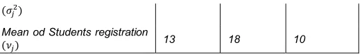
students. The data for the deterministic variables and the parameters for the stochastic random variables for the three colleges are given by Table 1.
College 1 College 2 College 3
No. of Professors (𝑥 ) 6 15 10
No. of Bachelors (𝑦 ) 29 27 2
No. of Masters (𝑦 ) 23 8 12
Mean of Annual Budget (𝜇 ) 17 28 12
(𝜎 )
Mean od Students registration
(𝜈) 13 18 10
Table 1: Inputs and outputs data for the three colleges
The annual students’ registration for the three colleges are independent, while the annual budget for the three colleges is a dependent variable as they are parts of one university. The dependency is described by the covariance as follows:
C𝑜𝑣(𝑥 𝑥 ) = 0.8 C𝑜𝑣(𝑥 𝑥 )
= 0.7 and C𝑜𝑣(𝑥 𝑥 ) = 0.6
Recall that, the aim of this example is to calculate the relative efficiency of the three colleges, within the same university. Let ϵ = 30% and hence 𝑒 = Φ (ϵ) = −0.5244.
All the below results are obtained by running a MATLAB script, which is available on Github for further simulations [24].
Case 1
In this case, we consider the annual budget follows normal distribution, while the annual students’ registration follows Poisson distribution. Then, according to Theorem 1, the relative efficiency score of the 𝑝-th college 𝜃𝑝 solves the following nonlinear optimization problem
𝑀𝑖𝑛𝑖𝑚𝑢𝑚(θ )
𝑠. 𝑡.
17λ + 28λ + 12λ − μ θ
≤ −0.5244 01.3(λ − δ θ )
+ 1.4(λ − δ θ ) + 1.3(λ − δ θ )
+ 2 .0.8(λ − δ θ )(λ − δ θ ) + 0.7(λ − δ θ )(λ − δ θ )
+ 0.6(λ − δ θ )(λ − δ θ )/1 /
𝑄 4√2ν (θ − λ ) 05
− 𝑄 4√2ν (θ − λ ) √2(13λ + 18λ + 16λ − ν λ )5
≤ 0.3
6λ + 15λ + 10λ ≤ 𝑥 θ
29λ + 27λ + 2λ ≥ 𝑦
23λ + 8λ + 12λ ≥ 𝑦
λ + λ + λ = 1
λ λ λ ≥ 0
(15 )
where 𝜇 𝜈 𝑥 𝑦 and 𝑦 are varying according to Table
1. Solving problem (15), for 𝑝 ∈ *1 2 3+, we obtain
• First college efficiency score: 𝜃1 = 100 %;
• Second college efficiency score: 𝜃2 = 98.36 %;
• Third college efficiency score: 𝜃3 = 100 %.
This means that first and third colleges are efficient while the second one is not efficient.
Case 2
In this case, the annual budget and the student registration inputs are assumed to follow normal distributions. Thus, we have two normal inputs and no Poisson inputs (i.e. |ℐ𝒩| = 2
and |ℐ | = 0). The variance of student registration variable corresponding to each college is equal to its mean and with no correlation among the colleges (i.e. 𝐶𝑜𝑣(𝑥 𝑥 ) = 0 for 𝑗 ≠ 𝑗). Then, according to Theorem 1, the relative efficiency score of the 𝑝-th college θ solves the following nonlinear optimization problem
𝑀𝑖𝑛𝑖𝑚𝑢𝑚(θ )
s.t.
17λ + 28λ + 12λ − μ θ
≤ −0.5244 01.3(λ − δ θ )
+ 1.4(λ − δ θ ) + 1.3(λ − δ θ )
+ 2 .0.8(λ − δ θ )(λ − δ θ ) + 0.7(λ − δ θ )(λ − δ θ )
+ 0.6(λ − δ θ )(λ − δ θ )/1 /
13λ + 18λ + 16λ − ν θ
≤ −0.5244 013(λ − δ θ )
+ 18(λ − δ θ )
+ 16(λ − δ θ ) 1 /
6λ + 15λ + 10λ ≤ 𝑥 θ
29λ + 27λ + 2λ ≥ 𝑦
23λ + 8λ + 12λ ≥ 𝑦
λ + λ + λ = 1
λ λ λ ≥ 0
(16)
where 𝜇 𝜈 𝑥 𝑦 and 𝑦 are given in Table 1. Solving problem (16), for 𝑝 ∈ 1 2 3 we obtain • First college efficiency score: 𝜃 = 100 %;
• Second college efficiency score: 𝜃 = 87.28%; • Third college efficiency score: 𝜃 = 100%.
3035
6 CONCLUSION
AND
FUTURE
WORK
DEA is a powerful tool, in management science, using mathematical programming to evaluate the performance, which is determined by the efficiency score, of different organizations, firms, products, etc. This efficiency measurement takes place in different applications like education, energy, agriculture, etc. Stochastic DEA models allow the inputs or outputs to be stochastic random variables. Only normal variables in such models were introduced in the literature. Variables which can be described by rate of flow usually follow Poisson or exponential distributions. These distributions have not been yet considered in stochastic DEA models. In this paper, the probability comparing two Poisson random variables is determined by difference of Marcum functions evaluated at different points related to the means of these variables. As a result, a deterministic model with non-identical random inputs, varying between either normal or Poisson distributions, is developed. In reality, this developed model gives flexibility in choosing the appropriate distribution for the input variables under consideration. The approach, used to formulate this novel model, can be used for output oriented stochastic DEA. Lastly, it is shown that misleading efficiency score will result from assuming all the stochastic inputs are normally distributed. For future work, inputs and outputs being random variables following distributions different than normal and Poisson can be considered. Moreover, the assumption on the dependency of Poisson random variables among the DMUs under analysis can be addressed in future studies.
7
REFERENCES
[1] T. Baležentis, I. Kriščiukaitienė, & A. Baležentis “A nonparametric analysis of the determinants of family farm efficiency dynamics in Lithuania,” Agricultural economics, 45(5), 589-599, 2014.
[2] R. D. Banker, A. Charnes, & W. W. Cooper “Some models for estimating technical and scale inefficiencies in data envelopment analysis,” Management science, 30(9), 1078-1092. Management Science. (1984) 30: 1078-1092. [3] A. Baricz, “Bounds for modified Bessel functions of
the first and second kinds," Proceedings of the Edinburgh Mathematical Society, 53(3), 575-599, 2010.
[4] J. Benicio & J. C. S. De Mello “Productivity analysis and variable returns of scale: DEA efficiency frontier interpretation,” Procedia Computer Science, 55(Itqm), 341-349, 2015.
[5] E. Bolandnazar, A. Keyhani & M. Omid “Determination of efficient and inefficient greenhouse cucumber producers using Data Envelopment Analysis approach,” a case study: Jiroft city in Iran. J Clean Prod; 79:108-15, 2014. [6] V. Charles & M. Kumar (Eds.) “Data envelopment
analysis and its applications to management’” Cambridge Scholars Publishing, 2013.
[7] W. W. Cooper, H. Deng, Z. Huang, & S. X. Li “Chance constrained programming approaches to technical efficiencies and inefficiencies in stochastic data envelopment analysis,” Journal of
the Operational Research Society, 53(12), 1347-1356, 2002.
[8] W. W. Cooper, H. Deng, Z. Huang, & S. X. Li “Chance constrained programming approaches to congestion in stochastic data envelopment analysis,” European Journal of Operational Research, 155(2), 487-501, 2004.
[9] A. O. Costa, L. B. Oliveira, M. P. E. Lins, A. C. M. Silva, M. S. M. Araujo, A. O. Pereira Jr, & L. P. Rosa “Sustainability analysis of biodiesel production: A review on different resources in Brazil,” Renewable and Sustainable Energy Reviews, 27, 407-412, 2013.
[10]B. E. El-Demerdash, I. A. El-Khodary, & A. A. Tharwat “Developing a stochastic input oriented data envelopment analysis (SIODEA) model,” International Journal of Advanced Computer Science and Applications, 4(4), 2013.
[11]A. Emrouznejad, & G. L. Yang “A survey and analysis of the first 40 years of scholarly literature in DEA: 19782016,” Socio-Economic Planning Sciences, 61, 4-8, 2018.
[12]H. L. Gan, & E. D. Kolaczyk, “Approximation of the difference of two Poisson-like counts by Skellam,” Journal of Applied Probability, 55(2), 416-430, 2018.
[13]S. J. Janke, & F. Tinsley, “Introduction to linear models and statistical inference,” John Wiley & Sons, 2005.
[14]F. Jones “Lebesgue Integration on Euclidean Space,” Jones and Bartlett publishers, pp. 527-529, 2001.
[15]D. Karlis, & I. Ntzoufras “Bayesian analysis of the differences of count data,” Statistics in medicine, 25(11), 1885-1905, 2006.
[16]M. Khodabakhshi, M. Asgharian, ] & G. N. Gregoriou “An input- oriented super-efficiency measure in stochastic data envelopment analysis: Evaluating chief executive officers of US public banks and thrifts,” Expert Systems with Applications, 37(3), 2092-2097, 2010.
[17]B. Khoshnevisan, H. M. Shariati, S. Rafiee & H. Mousazadeh “Comparison of energy consumption and GHG emissions of open field and greenhouse strawberry production” Renewable and Sustainable Energy Reviews, 29, 316- 324, 2014.
[18]S. K. Lee, G. Mogi & K. S. Hui “A fuzzy analytic hierarchy process (AHP)/data envelopment analysis (DEA) hybrid model for efficiently allocating energy R&D resources: In the case of energy technologies against high oil prices,” Renewable and Sustainable Energy Reviews, 21, 347-355, 2013.
[19]E. L. Lehmann Testing Statistical Hypotheses second edition John Wiley and sons, 1986.
[20]D. G. T. Reddy “Comparison and Correlation Coefficient between CRS and VRS models of OC Mines,” International Journal of Ethics in Engineering & Management Education, 2(1), 2348-4748, 2015.
[21]N. Mourad SIODEA with Normal and Poisson variables Source code, (Version 1.0),
[22]J. G. Skellam “The frequency distribution of the difference between two Poisson variates belonging to different populations,” Journal of the Royal Statistical Society. Series A (General), 109(Pt 3), 296-296, 1946.
[23]L. Simar & V. Zelenyuk “Stochastic FDH/DEA estimators for frontier analysis,” Journal of Productivity Analysis. 36 (1): 1-20, 2011.
[24]T. Song, Z. Yang, & T. Chahine “Efficiency evaluation of material and energy flows, a case study of Chinese cities,” Journal of Cleaner Production, 112, 3667-3675, 2016.
[25]X. P. Zhang, Y. X. Zhang, R. Rao & Z. P. Shi “Exploring the drivers to energy-related carbon emissions changes at Chinas provincial levels,” Energy Efficiency, 8(4), 699-712, 2015.