Volume 3, No. 3, May-June 2012
International Journal of Advanced Research in Computer Science
RESEARCH PAPER
Available Online at www.ijarcs.info
ISSN No. 0976-5697
A Priority Based Dynamic Round Robin with Deadline (PBDRRD) Scheduling Algorithm
for Hard Real Time Operating System
Rakesh Mohanty*, Shekhar Chandra Pradhan, Swarup Ranjan Behera
Department of Computer Science and Engineering Veer Surendra Sai University of Technology
Burla, Odisha, India
Abstract: In this paper, we have made a comprehensive study of variants of Round Robin (RR) scheduling algorithm existing in the literature for Real Time Operating System (RTOS). As per our knowledge there is no known efficient RR scheduling algorithm for Hard RTOS. Our study has been focused on a recently developed algorithm, known as Priority Based Dynamic Round Robin (PBDRR) scheduling algorithm. We have proposed a novel variant of PBDRR algorithm using deadline, which we call as PBDRRD algorithm. This algorithm can be efficiently used for Hard RTOS. We have made comparative performance evaluation of two algorithms i.e. PBDRR and PBDRRD by considering three cases of the input data set. We have computed the average turnaround time, average waiting time and number of context switches for both the algorithms using Gantt chart. Our experimental results show that performance of PBDRRD algorithm is better than that of PBDRR algorithm in all the three cases.
Keywords: Real Time Operating System, Scheduling, Round Robin, Dynamic Time Quantum, Intelligence Time Slice, Deadline.
I. INTRODUCTION
An operating system is a program that effectively and
efficiently manages the hardware and software resources of a computer system. A program in execution is called a process. Real Time Operating System (RTOS) is a special type of operating system in which a fixed time frame is
allotted for the execution of a process. RTOS finds
applications in fire alarm system, flight control system, embedded computing, space based defense systems, control of laboratory experiments, process control in industrial plants, robotics, air traffic control, telecommunications, military command and control systems.
A. Real Time Operating System:
RTOS can be classified into three types such as - Hard
RTOS, Soft RTOS and Firm RTOS. In Hard RTOS, the processes must meet their deadlines strictly before completion of execution, otherwise the system will fail. But in Soft RTOS, each process is associated with a deadline with some relaxation. In this case, the system may not fail
even if the deadline is not met,but the system’s quality of
services is degraded. In Firm RTOS, a low probability of missing a deadline can be accepted without the consequence of system failure. There are four important characteristics of RTOS such as determinism, responsiveness, user control and reliability. Determinism specifies that operations are to be performed at fixed predetermined times or within predetermined time intervals. Responsiveness is the time duration of servicing an interrupt by the operating system after an acknowledgment. It includes amount of time to begin execution of the interrupt and the amount of time to perform the interrupt. User control of an RTOS may involve activities like specifying priority and specifying
paging.The RTOS must be reliable in the sense that it
should not fail in adverse conditions. Scheduling of process in an RTOS involves act of selecting the order of allocation of Central Processing Unit (CPU) to the processes which are to be executed.
The scheduler is a component of operating system that
has to schedule the processes in such a way that they can finish their execution before their respective deadlines. Scheduling algorithms are designed to efficiently schedule the processes for execution. Scheduling algorithms can be
either pre-emptive or non-preemptive. In a pre-emptive
algorithm, a process is temporarily interrupted during execution and CPU is allocated to another process. In a non-preemptive algorithm a process cannot be interrupted until it completes its execution. Few basic terminologies and definitions related to operating system of scheduling are presented below.
B. Basic Terminologies:
Burst Time (TB) is the amount of CPU time a process
independently requires to complete its execution. Ready
queue is a queue where all the processes are entered before
allocation of CPU. Waiting Time (WT) is the amount of
time that a process spends waiting in the ready queue before execution. Turnaround Time (TAT) is the interval between the submission of process and its time of completion. Context Switch (CS) is the process of switching the CPU between two processes upon interrupt request by performing a state save of current process and a state restore of other.
Deadline (D) is the strict time constraint before which a
process has to finish its execution.
C. Scheduling Algorithms for RTOS:
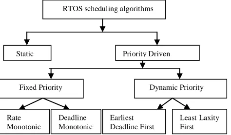
Figure 1. Classification of RTOS scheduling algorithm
RTOS scheduling algorithms can be classified into static
and priority driven. In static, the scheduling decisions are
made at compile time. A scheduling algorithm is said to be priority driven if and only if it satisfies a condition based on priority of processes. Priority driven can be of two types
such as fixed and dynamic. In fixed priority driven
algorithms, once a priority is assigned to a process it cannot be changed. In dynamic priority driven algorithm priority of an individual process may vary during execution. There exist two types of fixed priority driven algorithms such as Rate Monotonic (RM) and Deadline Monotonic (DM). In RM, priorities of processes are assigned based on their periods. The processes having shorter periods have higher priority than the processes having longer periods. The processes are sorted in the ready queue such that the period increases monotonically. In DM, processes are assigned priority according to their deadlines. The processes with shorter deadlines are assigned to higher priorities than the processes with longer deadlines. Dynamic priority driven algorithms are of two types such as Earliest Deadline First (EDF) and Least Laxity First (LLF). EDF uses deadline as the priority i.e. the process with earliest deadline has the highest priority. LLF algorithm assigns the highest priority to a process with least laxity. The laxity of a process is the difference between its deadline and remaining burst time. Some well-known and recently developed RTOS scheduling algorithms are presented below.
D. Literature Review:
Various RTOS scheduling algorithms have been extensively studied in the literature. A survey on contemporary RTOS has been presented in [1] which describes the necessary parameters that are required for
designing an RTOS. Some RTOS scheduling algorithms
are compared in [2]. A brief survey of RTOS along with static and dynamic scheduling has been done in [3].
Round Robin (RR) is one of the most effective
scheduling algorithms for RTOS [4]. Here each process is
assigned with a time slice or time quantum. A process is
executed for that time slice only and then preempted by another process, which is executed next for its time quantum and so on. Here the processes are executed in a circular round robin fashion. Simple RR scheduling algorithms have few limitations. They can’t be efficiently used in real time
systems since average waiting time and average turnaround time become more when the time quantum is very small.
The algorithm proposed in [5] overcomes the above
limitation by using variable time quantum, which operates in three phases. First phase consists of allocation of all processes to the CPU. These processes are executed by applying simple RR with initial time quantum. After completing first cycle, it doubles the time quantum in the next phase. Then it selects the process with shortest burst time from the ready queue and CPU is allocated to it. Then the CPU will be allocated to the next process with next shorter burst time. In third phase the execution cycle of phase one and phase two are repeated till the completion of execution of processes.
A modified version of RR scheduling algorithm has been proposed in [6] which introduces a concept called smart time slicing (STS). STS depends on three aspects such as priority, burst time and context switch avoidance time. Here the processes are arranged in increasing order of burst times which correspond to decreasing order of priorities. STS also depends on number of processes in the ready queue. The smart time slice is equal to the burst time of the middle process when numbers of processes are odd. If numbers of process are even then we consider the smart time slice according to the average CPU burst of all the running processes.
It is observed that a fixed time slice for all the processes during different cycles cannot improve the performance of a RR scheduling algorithm. Hence a new concept of intelligence time slice (ITS) has been proposed in [7]. ITS of each process is computed using different parameters like original time slice (OTS), priority component (PC), shortness component (SC) and context switch component (CSC). The OTS is the time slice given to any process if it deserves no special consideration. The PC value is 1 for the process having highest priority and 0 for the rest. The SC is computed based on the difference between the burst time of current process and the burst time of its previous process. If the difference is less than 0, then SC is assigned 1, otherwise SC is assigned to 0. For calculation of Context Switch Component (CSC) of a process, the parameters like PC, SC and OTS are added and then this result is subtracted from the burst time of that process. If the resulting value is less than OTS, then the same value is considered as CSC otherwise value of CSC is considered as 0.
Priority Based Dynamic Round Robin (PBDRR) algorithm has been proposed in [8]. It computes the ITS for each process as mentioned above and also uses the dynamic time quantum concept.
E. Our Contribution:
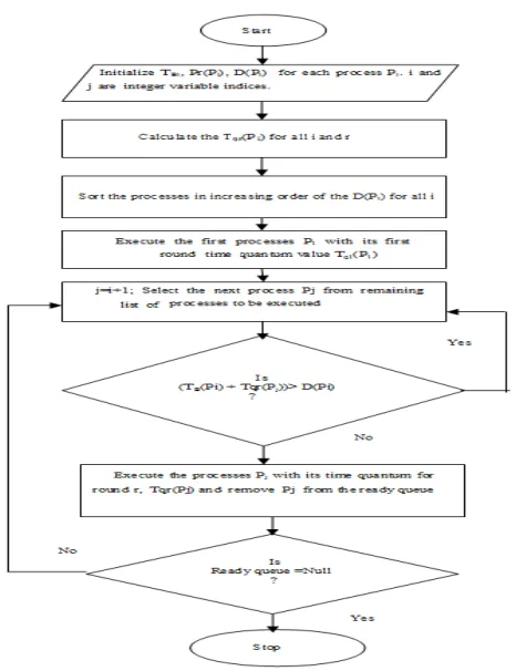
In our work, we have proposed a novel variant of the PBDRR algorithm using deadline which we call as PBDRRD. We have presented the pseudocode of our proposed PBDRRD algorithm as shown in Figure 2 and flowchart in Figure 3. We have made a comparative performance evaluation of two algorithms i.e. PBDRR and PBDRRD by considering three cases of the data set. We have computed the average TAT, average WT and number of CS for both the algorithms using Gantt chart. Our experimental results show that performance of PBDRRD algorithm is better than that of PBDRR algorithm.
F. Organization of Pape:r
Section I contains the Introduction along with literature review. The pseudo code, flowchart and illustrations of our proposed PBDRRD algorithm are given in section II. Section III contains the experimental results and performance comparisons of PBDRRD and PBDRR algorithm. Finally concluding remarks have been presented in section IV.
II.OURPROPOSEDPBDRRDALGORITHM
Our proposed algorithm is based on deadline parameter which is more significant for Hard RTOS. The process with earlier deadlines is given higher priority over processes with lower priorities. The pseudo code and flow chart of PBDRRD are presented in Figure 2 and Figure 3 respectively.
We have assumed that arrival time of all the process are the same. The priority is static in nature and assigned by the
user.Deadline of each of the processes must be greater than
or equal to the maximum burst time.
We have used the following notations in our pseudo code.
Notations:
Let n number of processes in the ready queue.
Pi process id, where i = 1, 2, 3,… n TBi burst time of Pi
Tqr (Pi) time quantum of Pi for round r D(Pi) deadline of Pi
Pr(Pi) priority of Pi
TRB (Pi) Remaining burst time of Pi
1. For i= 1, 2, 3 ….n, Calculate SC, PC, CSC and ITS of all Pi.
2.While(ready queue != null)
For i=1 to n do if( i ==1) then if(SC==0)then
Tq(Pi) =0.5 *ITS; Else
Tq(Pi) =ITS; End if Else
If(SC==0)then
Tq(Pi) = Tq(Pi-1) + 0.5* Tq(Pi-1) ; else
Tq(Pi) = 2 * Tq(Pi-1) ; End if
TRB(Pi) = TB( Pi) – Tq(Pi); If (TRB(Pi) <= 2 ) then
Tq(Pi)= TRB(Pi);
End for End while
3. Sort the processes Pi such that Pi < P j iff D(Pi) < D(Pj) for each i!=j
4. Assign CPU to P1 and execute the first process Pi for i=1 with its time quantum
for round one Tq1(P1).
5. j = i+1
Select the next process Pj from the sorted list of processes
6. if (TBi+Tqr(Pj))> D(Pi)
Go to step 5 Else
Execute process with Pj with Tqr(Pj)
7. if (ready queue != null) Go to step 5 Else Stop
Figure 2. Pseudo code for PBDRRD
Illustration of PBDRRD Algorithm:
Suppose there are 3 processes P1, P2 and P3 with burst times 6, 13, and 10 respectively. The user priorities of the processes are 2, 1 and 3 respectively. Their corresponding deadlines are 10, 20, and 30. OTS is taken as 3. The PCS are calculated as 0, 1, and 0. The SCs are found to be 0, 0 and 1. The CSCS values are calculated as 0, 0 and 0. ITSs are calculated as 3, 4, and 4. In the first round, the processes having SC as 1 are assigned time quantum same as ITS whereas the processes having SC as 0 are given the time quantum equal to the ceiling of the half of the ITS. So the processes P1, P2, P3 are assigned time quantum as 2, 2 and 4 respectively.
In next round, the processes having SC as 1 are assigned double the time slice of its previous round whereas the processes with SC equals to 0 are given the time quantum equal to the sum of previous time quantum and ceiling of the half of the previous time quantum. So for the second round the time quantum for three processes P1, P2 and P3 are 4, 3 and 6 respectively. Similarly time quantum is assigned to each process available in each round for execution.
After second round processes P1 and P3 have already completed so in third and fourth round the time quantum of P2 are 5 and 3 respectively. Then processes are sorted with increasing order of their deadline. So the final sequence is P1, P2 and P3 (here the sequence remains same). Subsequently P1 with time quantum value 2 is executed. Then P2 is executed with time quantum value 2. If we choose P3 as the next process to be executed then P1 is exceeding its deadline so P3 cannot be selected and again P1 is executed. Similarly the processes are executed in the order P2, P2, P2, P3 and P3.
III. EXPERIMENTSANDRESULTS
A. Data Set:
We have performed the experiments by taking three cases of input data set. The data set is based on increasing or decreasing or random order of burst times and deadlines of the processes. We have computed the average turnaround time and average waiting time of our proposed algorithm PBDRRD and PBDRR using Gantt chart.
B. Experiments Performed:
In our experiments we have taken five processes for case 1 and case 2 and four processes for case 3. In case 1, the 5 processes are taken in random order of burst time and deadlines. In case 2, we have taken 5 processes in decreasing order of burst time. In case 3, four processes are taken with random order of burst time and deadline. For simplicity we have taken either 5 or 4 processes for our experiments, though the algorithms are expected to show similar results for higher number of processes.
Case-1
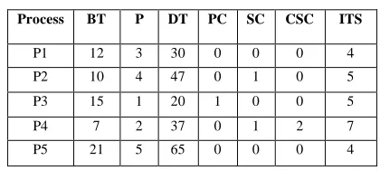
We have taken 5 processes P1, P2, P3, P4 and P5 with burst times 12, 10, 15, 7 and 21 respectively. The priorities
and deadlines associated with these processes are 3, 4, 1, 2, 5 and 30, 47, 20, 37, 65 respectively. different processes are computed as per their definitions. Case 1 results are represented in Table 1, Table 2, Table 3 and Figure 4, Figure 5.
Table 2. Computation of time quantum for different rounds
Process BT DT Round
Here the processes are arranged according to the increasing order of their deadlines. The time quantum for different rounds is calculated as shown in Table 2.
PBDRR
Figure 5. Gantt chart for PBDRRD of case 1
Table 3. Computation between PBDRR and PBDRRD
Method Avg. WT Avg. TAT
PBDRR 27.6 40
PBDRRD 26.4 39
Case-2
We have taken 5 processes P1, P2, P3, P4 and P5 with burst times 15, 10, 8, 5 and 3 respectively. The priorities and deadlines associated with these processes are 2, 1, 4, 5, 3
and 42, 25, 12, 27, 14 respectively. Here OTS value is taken
as 3. Case 2 results are represented in Table 4, Table 5,
Table 6 and Figure 6, Figure 7.
Table 4. Computation of ITS
Table 5. Computation of time quantum for different rounds
Process BT DT Round
1st 2nd 3rd 4th
P3 8 12 4 4 0 0
P5 3 14 3 0 0 0
P2 10 25 5 5 0 0
P4 5 27 5 0 0 0
P1 15 42 2 3 5 5
PBDRR
P1 P2 P3 P4 P5 P1 P2 P3 P1 P1
0 2 7 11 16 19 22 27 31 36 41
Figure 6. Gantt chart for PBDRR of case 2
PBDRRD
P3 P5 P3 P2 P2 P4 P1 P1 P1 P1
0 4 7 11 16 21 26 28 31 36 41
Figure 7. Gantt chart for PBDRRD of case 2
Table 6. Computation between PBDRR and PBDRRD
Method Avg. WT Avg. TAT
PBDRR 19.6 26.8
PBDRRD 13 21.2
Case-3
We have taken 5 processes P1, P2, P3 and P4 with burst times 8, 17, 10, and 12 respectively. The priorities and deadlines associated with these processes are 2, 3, 1, 4, and 10, 50, 23, 35 respectively. Here OTS is taken as 3. . Case 3 results are represented in Table 7, Table 8, Table 9 and Figure 8, Figure 9.
Table 7. Computation of ITS
Process BT P DT PC SC CSC ITS
P1 8 2 10 0 0 0 3
P2 17 3 50 0 0 0 3
P3 10 1 23 1 1 0 5
P4 12 4 35 0 1 0 3
Table 8. Computation of time quantum for different rounds
Process BT DT Round
1st 2nd 3rd 4th
P1 8 10 2 3 3 0
P3 10 23 5 5 0 0
P4 12 35 2 3 7 0
P2 17 50 2 3 5 7
PBDRR
P1 P2 P3 P4 P1 P2 P3 P4 P1 P2 P4 P2
0 2 4 9 11 14 17 22 25 28 33 40 47
Figure 8. Gantt chart for PBDRR of case 3
PBDRRD
P1 P4 P1 P1 P3 P4 P3 P4 P2 P2 P2 P2
0 2 4 7 10 15 18 23 30 32 35 40 47
Figure 9. Gantt chart for PBDRRD of case 3
Table 6. Computation between PBDRR and PBDRRD
Method Avg. WT Avg. TAT
PBDRR 22.5 34.25
PBDRRD 15.75 27.5
Figure10. Comparison of Avg. waiting time of PBDRR and PBDRRD
Process BT P DT PC SC CSC ITS
P1 15 2 42 0 0 0 3
P2 10 1 25 1 1 0 5
P3 8 4 12 0 1 0 4
P4 5 5 27 0 1 1 5
Figure 11. Comparison of Avg. turnaround time of PBDRR and PBDRRD
IV. CONCLUSION
From the experimental results we have observed that our proposed PBDRRD algorithm performs better than PBDRR in terms of average waiting time and average turnaround time. The number of context switches remains the same for both the algorithms PBDRR and PBDRRD. Though we have considered same arrival time for all the processes, different arrival time can be considered for different processes as a future work to design a more realistic RR scheduling algorithm.
V. REFERENCES
[1]. S. Baskiyar and N. Meghanathan, “A Survey on Contemporary Real Time Operating Systems”, Informatica, 29, 233-240, 2005.
[2]. A. Sandhu, “Performance Comparison of RTS scheduling algorithm”, International Journal of Computer Science and Technology, Vol 2, 391-396, 2011.
[3]. K. Ghosh, B. Mukherjee and K Schwan, “A Survey of Real Time Operating System” Technical Report, GIT-CC-93/18, 1994.
[4]. A. Silberschatz, P. B. Galvin and G. Gagne, 2006, “Operating Systems Concepts”, 7th edition, John Wiley and Sons, USA, ISBN: 9812-53-176-9, pp. 159-161.
[5]. A. Singh, P. Goyal and S. Batra ,“ An Optimized Round Robin Scheduling Algorithm for CPU Scheduling”, International Journal on Computer Science and Engineering Vol. 02, No. 07,2383-2385, 2010.
[6]. V. K. Dhakad, S. Hiranwal and K.C. Roy, “Adaptive Round Robin Scheduling using Shortest Burst Approach Based on Smart Time Slice”, International Journal of Computer Science and Communication Vol. 02, No. 02, 319-323, 2011.
[7]. C. Yaashuwanth and R. Ramesh ,“ Intelligent Time Slice for Round Robin in Real Time Operating System” International Journal of Research and Review in Applied Science Vol. 02, No. 02, 126-131, 2010.
[8]. Rakesh Mohanty, H. S. Behera, K. Patwari, M. Dash and M. L. Prasanna, “Priority Based Dynamic Round Robin (PBDRR) Algorithm with Intelligent Time Slice for Soft Real Time Systems” , International Journal of Advanced Computer Science and Application Vol. 02, No. 02,46-60, 2011.
[9]. S. M. Mostafa, S. Z. Rida and S. H. Hamad, “Finding Time Quantum Of Round Robin CPU Scheduling Algorithm in General Computing Systems using Integer Programming”, International Journal of Research and Review in Applied Science, 2010.
[10]. Rakesh Mohanty, M. Das, M. L. Prasanna and Sudhashree, “Design and Performance Evaluation of a New Proposed Fittest Job First Dynamic Round Robin (FJFDRR) Scheduling Algorithm” in International Journal of Computing Information System, Vol.2, No. 2, 23-27, 2011.