Volume 3, No. 5, Sept-Oct 2012
International Journal Of Advanced Research In Computer Science
RESEARCH PAPER
Available Online at www.ijarcs.info
ISSN No. 0976-5697
Performance quantification of Wireless Sensor Networks by implementing Zone Hybrid
Routing Protocol
Barjinder Singh*
M.Tech(CSE), R.I.E.T Phagwara Punjab Technical University
Kapurthala, India [email protected]
Er. Rishma Chawla
Assistant Professor, R.I.E.T Phagwara Department of Computer Science Engineering
Kapurthala , India [email protected]
Er. Suminder Kaur
Assistant professor , LKP Kapurthala Department of Computer Science Engineering
Kapurthala,India [email protected]
Abstract: A sensor network is composed of a large number of autonomous sensor nodes, which are densely deployed in the area of interest that is either inside the phenomenon or very close to it. Routing is an important operation, being the foundation of data exchanging between wireless devices. Zone Routing Protocol was the first hybrid routing protocol with both a proactive and a reactive routing components. ZRP was proposed to reduce the control overhead of proactive routing protocols and decrease the latency caused by route discovery in reactive routing protocols. ZRP defines a zone around each node consisting of a number of neighbourhoods. During this research work, the hybrid routing protocol ZRP is applied in wireless sensors and the corresponding performance of the network is measured in terms of overhead, delay and throughput. The main motive is to emphasis on routing process so that it can be enhanced with hybrid routing and the goals should be achieved. It is quantified that zone routing is more powerful than any other individual routing component and also during implementation of ZRP in Wireless Sensors some new scenarios are taken according to perspectives.
Keywords: Wireless Sensors, Zone Routing, ZRP, IARP, IERP, Hybrid Routing, Proactive Routing, Reactive Routing
I. INTRODUCTION
A Wireless Sensor Network is a self-configuring network of small sensor nodes communicating among themselves using radio signals, and deployed in quantity to sense, monitor and understand the physical world. The wireless sensor nodes are called motes, and are deployed within a special area to monitor a physical phenomenon. WSN devices have severe resource constraints in terms of energy, computation and memory [1]. An illustration that comprises Sensor nodes, their communication and topology is given in Figure1.
Figure1: Sensor nodes deployed, Gateway and nodes communication to the Server or Base Station [2]
Figure1: Sensor nodes deployed, Gateway and nodes communication to the Server or Base Station [2]
Wireless sensors sense the information, then all the data is collected by the gateway sensor node such as a sink node, which further relay it to the server or Base Station where data analysis is performed. Today, it has a very wide range of applications such as environment monitoring, forest fire detection, landslide detection, greenhouse monitoring etc[3]
In other words, it consists of a set of small devices with sensing and wireless communication capabilities. A huge number of these small devices configure the network and these motes have capabilities such as: Computational capabilities, Sensing capabilities and Communication capabilities.
There has been a long history of remote sensing. The evolution of the sensor network has been started from 1950s. During this period a system of long range acoustic sensors called Sound Surveillance System (SOSUS) has been deployed in the deep basins of the Atlantic and Pacific oceans for sub-marine surveillance.
Networks of air defence radars can be regarded as an example of networked large scale sensors. Both the ground based radar systems and Airborne Warning and Control System (AWACS) planes are integrated in to such networks to provide all whether surveillance, command, control and communications. In 1980s and 1990s, the Co-operative Engagement Capability (CEC), was developed as a military sensor network, in which information gathered by multiple
Server
Sensor Node
radars was shared across the entire system. This was used for a consistent view of battle field.
The characteristics of the wireless sensor network: a WSNs consist of a large number of low power, low cost and multi function sensor network. These sensor nodes are small in size .But equipped with sensor, embedded microprocessor and radio transceivers.
Dense node deployment: the sensor nodes are used densely deployed in a field of interest. A number of sensor nodes in a sensor network can be several orders of magnitude higher than in a MANET [2].
Self configurable: The sensor nodes are deployed usually randomly without careful planning. Once deployed, sensor nodes have to autonomously configure themselves into a communication networks.
Battery-power sensor node: the sensor node powered by battery. They are deployed in a hostile environment, where it is very difficult to change or recharge the batteries.
Routing is very important process in wireless sensors. Zone routing is divided into two main components which are IARP and IERP. IntraZone protocol is a proactive routing protocol. IARP is used inside routing zones. A route to a destination within the local zone can be established from the source's proactively cached routing table by IARP.
The motivation for this work includes the research on already implemented proactive and reactive routing protocols in wireless sensor networks. This brings an idea to my mind that if these isolated protocols are implemented then why not we can combine their features and then implement it in WSN. Then I come to know that Zone routing is an important concept and it was implemented in Ad-hoc networks. With the proper guidance from my Guides, I made a detailed research on it and then implement ZRP in wireless sensors and quantify its performance. It was really an interesting and systematic journey which incorporates a lot of hard work, effort, determination and creativity.
II. PROACTIVEANDREACTIVEROUTING
A reactive routing protocol tries to find a route from S to D only on-demand i.e., when the route is required, for example, DSR and AODV are such protocols. The main advantage of a reactive protocol is the low overhead of control messages. A reactive routing protocol tries to find a route from S to D only on-demand i.e., when the route is required, for example, DSR and AODV are such protocols.The main advantage of a reactive protocol is the low overhead of control messages. However, reactive protocols have higher latency in discovering routes [4].
It is possible to exploit the good features of both reactive and proactive protcols and the Zone routing protocol does that. The proactive part of the protocol is restricted to a small neighbourhood of a node and the reactive part is used for routing across the network. This reduces latency in route discovery and reduces the number of control messages as well.
Each node “S“ in the network has a routing zone. This is the proactive zone for S as S collects information about its routing zone in the manner of the DSDV protocol. If the
radius of the routing zone is “r“, each node in the zone can be reached within r hops from S. The minimum distance of a peripheral node from S is r (the radius). All nodes except L are in the routing zone of S with radius 2 (illustrated in Figure2) [5].
The routing in ZRP is divided into two parts :
A. Intrazone routing:
It is defined as the routing where the packet is sent within the routing zone of the source node to reach the peripheral nodes. Intra-zone protocol [5] is a proactive routing protocol. IARP is used inside routing zones. A route to a destination within the local zone can be established from the source's proactively cached routing table by IARP [1].
B. Interzone routing:
It is defined as the routing Where the packet is sent from the peripheral nodes towards the destination node. IntErzone [5] Routing Protocol (IERP) is a global reactive routing component of ZRP. It determine the proper route only when required (on-demand) [1].
Figure2:sensor nodes with in and outside Zone
Each node collects information about all the nodes in its routing zone proactively. This strategy is similar to a proactive protocol like DSDV. Each node maintains a route table for its routing zone, so that it can find a route to any node in the routing zone from this table.In the original ZRP proposal, intrazone routing is done by maintaining a link state table at each node. Each node periodically broadcasts a message similar to a hello message. We call this message as a zone notification message.
Suppose the zone radius is r, for r>1,A hello message dies after one hop, i.e., after reaching a node´s neighbours. A zone notification mesage dies after “r“ hops, i.e., after reaching the node´s neighbours at a distance of “r“ hops.
Each node receiving this message decreases the hop count of the message by one and forwards the message to its neighbours. The message is not forwarded any more when the hop count is zero. Each node P keeps track of its neighbour Q from whom it received the message through an entry in its link state table. P can keep track of all the nodes in its routing zone through its link state table.
is within the routing zone of S, the routing is completed in the intrazone routing phase. Otherwise, S sends the packet to the peripheral nodes of its zone through bordercasting.
The bordercasting to peripheral nodes can be done mainly in two ways, First is by maintaining a multicast tree for the peripheral nodes. S(source) is the root of this tree. [6] Otherwise, S maintains complete routing table for its zone and routes the packet to the peripheral nodes by consulting this routing table. S sends a route request (RREQ) message to the peripheral nodes of its zone through bordercasting. (illustrated in Figure4) [7].
Each peripheral node P executes the same algorithm. First, P checks whether the destination D is within its routing zone and if so, sends the packet to D. Otherwise, P sends the packet to the peripheral nodes of its routing zone through bordercasting. (illustrated in Figure3)
Figure3: source to destination communication through various nodes[3]
If a node P finds that the destination D is within its routing zone, P can initiate a route reply. Each node appends its address to the RREQ message during the route request phase. This is similar to route request phase in DSR. This accumulated address can be used to send the route reply (RREP) back to the source node S. (ilustrated in Figure5).
An alternative strategy is to keep forward and backward links at every node´s route table similar to the AODV protocol. This helps in keeping the packet size constant. A RREQ usually results in more than one RREP and ZRP keeps track of more than one path between S and D. An alternative path is chosen in case one path is broken. ZRP: Example with Zone Radius , r = 2
Zone radius is the parameter used to create zones over the deployment area. In the following figure there are five zones are created, S is source , D is destination and all other are border nodes.
Figure4: Route Request [8]
Denotes route request, S performs route discovery for D
As illustrated in Figure5, E knows route from E to D, so route request need not to be forwarded to D from E.
Figure5: Route Reply [2]
Denotes route reply
Figure6: Data Transfer [3]
Denotes route taken by data
After collecting all the information regarding the desination , the Source send all the packets and the packets follow the discovered route. It is conspicuous in Figure6.
III. ARCHITECTUREOFZRP
The Zone Routing Protocol, as its name implies, is based on the concept of zones. A routing zone is defined for each node separately, and the zones of neighbouring nodes overlap. The routing zone has a radius “r” expressed in hops. The zone thus includes the nodes, whose distance from the intended node is at most r hops.
ZRP
Inter process comm..
Packet flow
Figure7: ZRP architecture [4]
IARP IERP
BRP
NETWORK LAYER
The relationship between the components is illustrated in Figure7. IARP, IERP and BRP are defined on Network layer and NDP is defined on the MAC Sub-layer of Data Link layer. Route updates are activated by NDP, which notifies IARP, when the neighbour table is updated. IERP [5] uses the routing table of IARP to respond to route queries. IERP forwards queries with BRP. BRP [5] uses the routing table of IARP to guide route queries away from the query source. [6]
In order to detect new neighbor nodes and link failures, the ZRP relies on a Neighbor Discovery Protocol (NDP) provided by the Media Access Control (MAC) layer. NDP transmits “HELLO” beacons at regular intervals [1]. After receiving a beacon, the neighbor table is updated. Neighbors, for which no beacon has been received within a specified time, are removed from the table. If the MAC layer does not include a NDP, the functionality must be provided by IARP. [5]
IV. PROBLEM FORMULATION
Routing is the process of selecting optimal pathway over the network to route the traffic. In case of Table Driven Routing Protocol or Proactive routing each node maintains one or more tables containing routing information to every other node in the network. Tables need to be consistent and up-to-date view of the network. Updates propagate through the network. E.g. DSDV, OLSR, WRP etc [9].
On the other hand, Source Initiated On demand routing protocol is Reactive in nature. It uses on-demand style, and creates routes only when it is desired by the source node. When a node requires a route to a destination, it initiates a route discovery process [10]. Route is maintained until destination becomes unreachable, or source no longer is interested in destination. E.g.: AODV, DSR etc [11]. ZRP is a hybrid protocol that incorporates the merits of on demand and proactive routing protocol, which provides efficient and fast discovery of route [12]. It limits the scope of the proactive procedure only to the node’s local neighbourhood. So in such a way ZRP protocol reduces the waste associated with routing update traffic of proactive routing to the limited number of zone members. On the other hand, performance and throughput becomes efficient as the querying is performed on selected nodes in the network, rather than flooding queries all over the network [3].
ZRP is already implemented in wireless ad hoc networks and this hybrid protocol generates better results rather than the individual proactive or reactive components [13]. So, this brings an idea in my mind that why not I can implement hybrid routing protocol ZRP in wireless sensor networks. I implemented it and quantify its performance in WSN, and it really became more efficient routing protocol than others as well as previous implementations [1].
V. METHODOLOGY
a. First of all obtain the co-ordinate position of complete deployment area.
b. Then Compute the deployment area. Divide the deployment area into n equal no. of zones.
c. Obtain the co-ordinate point for each sensor node with in the deployment area using hello packets. d. Now based on the co-ordinate positions of sensor
nodes divide the deployment area into zones in a way that the concentration of a sensor nodes with in each zone should be approximately same.
e. Associate each node-id with its zone-id. Each node with in the zone will now send hello packets & form communication link with the neighbors found in its zone.
f. From this step we will obtain a mesh out of which we can obtain a best tree for routing packets from source to destination.(the best tree can be obtained using min spanning tree).
g. Compute the energy level of each node within the zone [14].
h. Based on the energy level the nodes with the highest energy level will now act as root of the tree. The root node will act as sink node as well as the Bordercast node [15].
i. This sink node will aggregate the data and transfer it according to the algorithms implemented.
j. The Source node communicates to the Sink node and it further convey to the destination node when the data is to be transferred within the zone by using IARP.
k. The Sink nodes communicate to each other with in the deployment area using IERP to transfer data, rather than to other relay nodes, which reduces the overhead and delay.
l. The root node or Sink node will communicate or form a link with the base station, when the Destination-id does not exist in the created zones. m. The Base Station will communicate to all the Sink
nodes of each and every zone, when the Source-id does not exist in the created zones, means Source is somewhere outside the created zones, but the destination exists in the created zones.
n. When Source as well as Destination exists outside (unknown) the created zones, the system discards that data and terminates.
VI. PROPOSED ALGORITHM
A. Intrazone routing protocol Algorithm:
Yes
No
No Yes
Figure8: IARP create update message
All node in the zone receives the broadcast message. It first extract the routing information from the souce header. Then it updates or adds the routing entry to the source in its RT table. As the source is directly reachable , next node in the entry should be the source address and distance is one hop. Furthermore , this source address will become next node in the path. IARP Receiving update algorithm is shown as in Figure9.
Yes
No
Figure9: Receive IARP update message
B. Interzone Routing Protocol Algorithm:
Whenever a destination is not in one’s local routing zone, an IERP route discovery begins. First, the program searches the query table to see whether the destination query exists. If the query exists and the route path is known, a “Ready to Send Packets” message is return; if the query exists but no route path is available, the procedure must wait until the reply message of previous query is returned or is time out; otherwise a route to the destination must be queried. IERP will form a query message, after recording the query information in query table and ET table, and setting the timer for maximum waiting time out for getting the query reply , the query message is broadcasted via the IARP protocol. The returned reply message will include an accumulated route path to the destination. A single query may return multiple route path replies; the best route is selected for transfer. If the query waiting time count is timeout, which means the destination can’t reach or delay is too long, a “destination can’t be found” error message is produced after the query entry in query table is erased.
yes
yes
No
No
Yes
Figure10: IERP message sending
In the query processing, first, the node needs to check the query information in its ET table. If the query has been early detected, early termination will occur to end the query forwarding. Otherwise, if the query is first time received, it Start
Get more entry from RT(Routing table)
Is out of date Entry
Is border node (distance>=rad)
Entries count +1
Delete entry in table Put source info in message
header
Calculate time stamp
Put this into message (distance+1,
timestamp) Using IARP protocol to
broadcast update message
Get replied routing path
Select a best route path
Put path into query table
Return “ready” message to caller Timeout
Delete entry in query table
Return error message to caller
End
Get source information (Saddress, number of entry)
Insert /update Saddress entry
Entries= 0?
Node addr = this node?
Update new entry in table
End
Number of entry - 1 Get next entry
Start
Start
Already queried??
Set query waiting timeout
Create IERP query
Record query info in (query table or ET table)
Send query to IARP
Waiting for reply message
will record the query information in ET table. Next, after decreasing the hop count by one, the node checks if the query reaches a border node. If not, this interior node will re-broadcast the query message to its neighboring nodes. If the query reaches a border node, the border node will check if the destination is reachable within its local zone. If the border node can’t find the destination in its local routing table (unreachable) , it resets hop count to the zone radius and overwrites sender with this border node address, then continue to broadcast this query. If the destination is within the local zone of this border node, it will invoke the procedure to create and send a reply message back to the querying source. Certainly, a query can’t spread out the entire network forever; it must be dropped when it reaches a zone count limit setting in the source query message.
y
Intermediate node n
Border Node
y
n
y
n
Figure11: IERP Process Query
Route reply message is to be returned back to the queried source by the border node within the zone. The route in reply message accumulates the whole path from source to destination. A route discovery procedure finishes after the accumulated information is stored in query table.
yes
Figure12: IERP Reply
VII. EXPERIMENTAL RESULT
Simulation is performed in MATLAB. Deployment area is displayed according to given inputs. The deployment area is measured according to the parameters length and breadth. The scenario is dynamic in nature that is nodes may vary in zones.
Figure13: Deployment of equal number of sensor nodes in the created zones
The above diagram shows the positioning of sensor nodes in the created zones. The same number of sensors is deployed in each zone. In our scenario we have taken 7 sensors in each zone. Red color node acts as a sink node as well as the border node in each zone, that aggregates, identifies the particular destination in its zone or it communicates with other sinks according to algorithm for that particular destination.
Received Query Message
Early Detected?
Record query info (sAddr, dAddr, sender, time) in ET Table
Hopcount-1=0? (query reach border
node)
Destination within local zone?
Broadcasting query
End
Create / send reply message
Replace sender with this border node
(Zone-count)-1 , hop count=radius
Forwarding routing query Zone Count-1
> 0?
B
Destination within zone?
Add thisNode and destination address in routing path Create reply message
Send reply to sender Reset zone count to 2
(Route Length)
Figure14: Transfer of data with in the zone using IARP
The diagram shows the transfer of data with in the zone through IARP component of ZRP. The source node (206) communicates to the sink node through the intermediate relaying nodes. The sink node identifies the destination with in the zone using algorithmic part. It becomes Green, when it receives a request and finds the path up to the destination node (202).
Figure15: Transfer of data between different zones using IERP
The data is transferred outside the zone by using IERP. In the above graph the source sensor node communicates to the sink node, and it checks for the destination outside the zone by communicating to the sink nodes (border nodes) in other zones as per the algorithm. The sink node in the local zone transfer the request to its neighbour zone’s sinks.
First of all, the sender sends the data to the sink or the border node of second zone as illustrated, it broadcasts the data to the border nodes of its neighbours. They will check for the destination. If it is not there they will communicate further with other zone’s sink node and the process will continue until it reaches to the destination. When the sink node in the particular zone recognizes the sensor, it replies to the source sink node and data is to be transferred.
When the destination is out of zones created in the deployment area, the destination is first found out in all the zones and when it does not finds, the last zone sink node or border node communicates to the Base station, because the destination may be exist in some outer deployment area.
Figure16: Communication to the Base Station when Destination is Out of zones
In the above illustration, the source node is 204 and the destination node is 902. We have created only seven zones and the sensor-id 902 is not present in these zones. So in such a case when source is with in the zone and destination is outside the created zones then the sink of the last zone communicates to the base station.
Figure17: communication through Base station when Source is in some unknown zone
When the source exists in some unknown zone but the destination exist in our created zones. It means the data comes from some outside zone. Then the base station communicates to the sink of all the zones and establishes a connection and creates a database. In this scenario if the packet comes from outside area for the known destination zone the base station will send the request to all the sinks, the particular sink recognizes that the destination is in its zone, it becomes green and it will forward data to the specific destination according to its records of all the sensors in that zone.
In the above Scenario, the source node is present out of zones having Sensor-id is 904 and the destination is 202. Base Station transfers the request to all the sinks of in every zone. The specific sink node becomes green and it forwards the data to 202.
VIII. RESULTSANDANALYSISOFIMPLEMENTED ALGORITHM
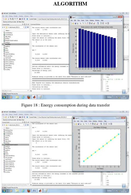
Figure 18 : Energy consumption during data transfer
Figure19: Graph shows zone radius versus Energy
[image:8.612.34.282.509.669.2]As the Zone radius increases, the size of each zone increases due to which processing power in each zone varies and when the zone radius increases energy required in each zone also increases [16].
Figure 20: Graph shows the result comparison of Throughput and packet delivery ratio
The Figure20 shows that as the packet generation interval increases the throughput of the system improves and it never degrades. The yellow line represents the packet
generation rate and the red line shows the corresponding Throughput of the system.
Table I : Showing Packet Generation Interval and corresponding Packet Delivery Ratio and Throughput
Packet Generation Interval(ms)
Packet Delivery Ratio
Throughput (kbps)
02 1060 1160
04 1100 1220
06 1130 1260
. . .
12 1205 1330
The Table I shows that as the packet generation interval increases packet delivery ratio increases and correspondingly throughput of the system moves up. When the interval is 2ms the packet delivery ratio is 1060 which is less as compare to ratio when interval is 12ms. At the start packets may loss but it improves as the interval increases. Throughput of the system may degrade only in the case packet delivery ratio declines or in case when the resources are underutilized.
Figure21 : Graph shows the results of parameter overhead in performance quantification
It is conspicuous that as the zone radius increases the additional overhead is there. The theoretically calculated overhead is compared to the taken simulation results. Zone radius is the parameter that defines a zone in the deployment area. In our case the length and breadth parameters are used to calculate the deployment area. The fixed size of each zone is taken as the zone radius.
So as a result of which lesser congestion will be there that reduces delays and increases the throughput as well as goodput of the system.
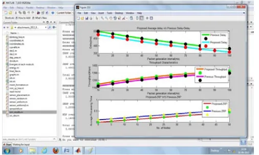
Figure22: Subplots shows the comparison results of Purposed and Previous implementations
The above graphs show the comparisons of performance quantification parameters delay, throughput and average processing time for proposed and previous systems. The below tables statistics prove it as the result details [17].
Table 2: Showing Packet Generation rate and corresponding Previous and Proposed Delay
Packet Generation Rate
Delay Previous(ms)
Delay Proposed(ms)
10 500 475
20 485 460
30 470 435
. . .
100 380 360
Table 3: Showing Packet Generation rate and corresponding Previous and Proposed Throughput
Packet Generation Rate
Throughput Previous
Throughput Proposed
10 1120 1150
20 1135 1170
30 1150 1190
. . .
[image:9.612.34.287.97.248.2]100 1250 1290
Table 4: Showing Number of nodes and corresponding Previous and Proposed Average Processing Time
Number of Nodes
Avg. Processing Time Previous
Avg. Processing Time Proposed
5 0.15 0.04
10 0.18 0.08
15 0.22 0.12
. . .
50 0.55 0.45
The above table shows that as the number of nodes increase in a zone, the average processing time also increases. When number of nodes are 5, the average
processing time is 0.04 in simulation results which is much better than the previous result for the same number of nodes. When there are up to 50 nodes in each zone the processing time improves slightly but significantly.
IX. CONCLUSION
In this research work, we propose Zone Routing Protocol for the WSNs which over passes the features of its implementation in mobile ad-hoc networks. we drawn that ZRP gives better performance with WSNs rather than using mobile ad-hoc network. Specifically, zones created in ZRP uses low energy and produces better throughput with good packet delivery ratio. We come to a conclusion, by this implementation results that using ZRP with WSNs produce better results than theoretical analysis as well as the other proactive and reactive routing protocols. To sum up, we would say, better throughput, packet delivery ratio, less overhead, less delay is there. Also less control information is relayed to route discovery. As a result of which effective performance generated on the network.
X. FUTURE SCOPE OF WORK
It is interesting to see the performance of ZRP in large and realistic scenario. Also in future, we can work on required energy efficiency, security scalability, prolonged network life time and load balancing. We applied the ZRP in WSNs which was earlier used with mobile ad-hoc network and the results achieved are much better than Ad hoc. So by implementing hybrid routing in WSN, we can reduce the overhead, delay etc, further one can implement enhanced hybrid ZRP protocol to achieve better performance on the network. Advanced Energy efficiency protocols can be used with hybrid routing to make the network more energy efficient. We can consider other parameters also, to improve the performance of wireless sensor networks.
XI. REFERENCES
[1]. Brijesh Patel and Sanjay Srivastava Dhirubhai Ambani Institute of Information and Communication Technology Gandhinagar 382 007, India “Performance Analysis of Zone Routing Protocols in Mobile Ad Hoc Networks” Digital Object Identifier: Publication Year: 2010 , Page(s): 1 – 5
[2]. Nicklas Beijar Networking Laboratory, Helsinki University of Technology P.O. Box 3000, FIN-02015 HUT, Finland “Zone Routing Protocol (ZRP)”
[3]. Yuki Sato*, Akio Koyama*, Leonard Barolli*** Department of Informatics, Graduate School of Science and Engineering,Yamagata University, Japan “A Zone Based Routing Protocol for Ad Hoc Networks and Its Performance Improvement by Reduction of Control Packets
Identifier 2010 , Page(s): 17 - 24
[4]. Prasun Sinha, Co-ordinated Sciences Laboratory, University of Illinois, Urbana Champaign “Scalable Unidirectional Routing with Zone Routing Protocol (ZRP) Extensions for Mobile Ad-Hoc Networks”
[5]. Jan Schaumann “Analysis of the Zone Routing Protocol”
[6]. Lotf, J.J.; Ghazani, S.H.H.N
[7]. Changjiang Jiang; Min Xiang; Weiren Shi “ Overview of cluster-based routing protocols in wireless sensor networks ” Digital Object Identifier: Publication Year: 2011 , Page(s): 3414 - 3417
[8]. Mohammed Ismail, @ Dr. M.Y. Sanavullah *Research Scholar, Department of Electronics, Vinayaka Mission University, Salem “Efficient On-Demand Routing Protocols to Optimize Network Coverage in Wireless Sensor Networks”
[9]. Charles E. Perkins, “Destination Sequence Distance Vector Protocol,” AdHoc Networking, ISBN 0-201-30976-9, pp. 53-74.
[10]. P.Kuppusamy Dept. of Computer Science and Engineering Vivekananda College of Engineering for Women Namakkal, India “A Study and Comparison of OLSR, AODV and TORA Routing Protocols in Ad Hoc Networks”
[11]. SreeRangaRaju*, Jitendranath Mungara**,*Department of Telecommunication Engineering, Bangalore Institute of Technology Bangalore, India “ZRP Versus AODV and DSR: A Comprehensive Study on ZRP Performance Using Qualnet Simulator”
[12]. K.P. Vijayakumar, P. Ganeshkumar and M. Anandaraj, Department of IT, PSNA College of Engg. & Tech., Dindigul, TamilNadu, India “Review on Routing Algorithms in Wireless Mesh Networks”
[13]. Fabian Nack Institute of Computer Science (ICS), Freie Universität Berlin “An Overview on Wireless Sensor Networks”
[14]. Kamal BeydounLIFC, University of Franche-Comté “Energy-Efficient WSN Infrastructure” published in Distibuted collabotative sensor networks USA in 2008.
[15]. Xin Liu, Quanyu Wang and Xuliang Jin Department of Computer Science and Technology Beijing Institute of Technology “An Energy-efficient Routing Protocol for Wireless Sensor Networks”
[16]. Usama Ahmed, Faisal Bashir Hussain,(2011) “Energy Efficient Routing Protocol for Zone Based Mobile Sensor Networks”.