Breast Cancer Prediction System using Feature Selection and Data Mining Methods

(1)

!

"

#"#

$ % %#

&

''' (

Breast Cancer Prediction System using Feature Selection and Data Mining Methods

Gayathri Devi.S

Senior Lecturer

Department of Information Technology Coimbatore Institute of Engineering and Technology

[email protected]

Abstract: Cancer is the second most common cause of death worldwide with an estimated 7.9 million of deaths in 2007. This number is projected to rise further and reach 12 million deaths in 2030 which makes cancer a major public health issue. Early diagnosis and more recent tools of managing cancer have shown to significantly improve the chances of survival and have brought new hope to patients. The identity of cancer from various factors or symptoms is a multifaceted issue which is not free from false presumptions often accompanied by volatile effects. In this paper, we have proposed three different feature selection method rank search, genetic search and greedy step wise search methods to identify the potential attributes from the Breast Cancer dataset using the classification of heart attack using data mining techniques. This breast cancer databases was obtained from the University of Wisconsin Hospitals, Madison from Dr. William H. Wolberg. Attributes 2 through 10 have been used to represent instances. Each instance has one of 2 possible classes: benign or malignant. Number of instances: 699 we have investigated six different classification data mining techniques such as BayesNet, AttributeSelectedClassifier, J48, ClassificationviaRegression, Logistic, and OneR. The result shows that the three different set of potential attributes are obtained through rank search, genetic search and greedy step. It is observed that the performance and the time taken by each classification algorithms are significantly improved after feature selection and the bayesnet classifier outperforms the remaining algorithms used in this paper.

Keywords:Breast Cancer, Data Mining, Classification, BayesNet, ClassificationviaRegression, Logistic, Rank Search, Genetic Search , Greedy Stepwise Search

I. INTRODUCTION

Breast cancer occurs when a malignant (cancerous) tumor originates in the breast. As breast cancer tumors mature, they may metastasize (spread) to other parts of the body[1]. The primary route of metastasis is the lymphatic system which, ironically enough, is also the body's primary system for producing and transporting white blood cells and other cancer-fighting immune system cells throughout the body[2]. Metastasized cancer cells that aren't destroyed by the lymphatic system's white blood cells move through the lymphatic vessels and settle in remote body locations, forming new tumors and perpetuating the disease process. Though some of these risk factors are unavoidable and uncontrollable, some of them are very avoidable, making it possible for people to take action so as to minimize their cancer risk[3]. Even a minimized risk is still a risk, however. There is no way to pre-determine whether a person will get breast cancer until they have either been diagnosed with it or they have lived a breast-cancer free lifetime [4].

Data Mining and Statistics Analysis is the search for valuable information in large volumes of data. It is now widely used in health care industry [5] [6]. Especially breast cancer is the second most cause of cancer and the second most dangerous cancer. The best way to improve a breast cancer victim’s chance of long-term survival is to detect it as early as possible

These records are cleaned and filtered with the intention that the irrelevant data from the warehouse would be removed before mining process occurs. The aim of this paper is to predict the Breast Cancer effectively by applying the attribute subset evaluator namely Consistency Subset Evaluator and the searching methods used are Rank search, Greedy Stepwise forward Search and Genetic Search. These three methods produce 6, 5 and 4 significant attributes for

classification respectively. Using these significant attributes the classification of dataset is performed using J48, Bbayesnet, Logistic, Classification via regression and Attribute Selected Classifier.

The remaining sections of the paper are organized as follows: In Section 2, a brief review of some of the works on Breast Cancer diagnosis is presented. An introduction about the Breast Cancer and its effects are given in Section 3. In Section 4 description about the dataset is produced. The section 5 explains the framework of the proposed model. The extraction of significant attributes from Breast Cancer data warehouse is detailed in Section 6. The classification methods used for predicting the Breast Cancer is explained in Section 7. Estimation of model performance is shown in the Section 8. The experimental results are described in Section 9. The conclusions are summed up in Section 10.

II. RELATEDWORK

(2)

Leukemia Cell Classes [12] in this paper using data mining techniques, a subset (1400) of compounds from the large public National Cancer Institute (NCI) compounds data repository has been studied.

III. BREASTCANCERDISEASE

The human body is composed of many millions of tiny cells, each a self-contained living unit. Normally, each cell coordinates with the others that compose tissues and organs of your body. One way that this coordination occurs is reflected in how your cells reproduce themselves. Normal cells in the body grow and divide for a period of time and then stop growing and dividing. Thereafter, they only reproduce themselves as necessary to replace defective or dying cells. Cancer occurs when this cellular reproduction process goes out of control. In other words, cancer is a disease characterized by uncontrolled, uncoordinated and undesirable cell division. Unlike normal cells, cancer cells continue to grow and divide for their whole lives, replicating into more and more harmful cells.

The abnormal growth and division observed in cancer cells is caused by damage in these cells' DNA (genetic material inside cells that determines cellular characteristics and functioning). There are a variety of ways that cellular DNA can become damaged and defective. For example, environmental factors (such as exposure to tobacco smoke) can initiate a chain of events that results in cellular DNA defects that lead to cancer. Alternatively, defective DNA can be inherited from your parents.

As cancer cells divide and replicate themselves, they often form into a clump of cancer cells known as a tumor. Tumors cause many of the symptoms of cancer by pressuring, crushing and destroying surrounding non-cancerous cells and tissues.

Tumors come in two forms; benign and malignant. Benign tumors are not cancerous, thus they do not grow and spread to the extent of cancerous tumors. Benign tumors are usually not life threatening. Malignant tumors, on the other hand, grow and spread to other areas of the body. The process whereby cancer cells travel from the initial tumor site to other parts of the body is known as metastasis. In this paper classification of the dataset is performed based on benign and malignant.

IV. DATASETDESCRIPTION

This breast cancer databases was obtained from the University of Wisconsin Hospitals, Madison from Dr. William H. Wolberg[13,14,15,&16]. Samples arrive periodically as Dr. Wolberg reports his clinical cases. The database therefore reflects this chronological grouping of the data. This grouping information appears immediately below, having been removed from the data itself:

This breast cancer databases obtained from the University of Wisconsin Hospitals, Madison from Dr. William H. Wolberg has the attributes listed in the table. Attributes 2 through 10 have been used to represent instances. Each instance has one of 2 possible classes: benign or malignant. Number of instances: 699

A. Number of Attributes : 10 plus the class attribute B. Attribute Information: (class attribute has been moved to

last column)

Table I. List of Attributes

# Attribute Domain

1 Sample Code Number Id number 2 Clump Thickness 1-10 3 Uniformity of Cell Size 1-10 4 Uniformity of Cell Shape 1-10 5 Marginal Adhesion 1-10 6 Single Epithelial Cell Size 1-10 7 Bare Nuclei 1-10 8 Bland Chromatin 1-10 9 Normal Nucleoli 1-10

10 Mitoses 1-10

11 Class (2 for benign, 4 for malignant)

C. Missing attribute values: 16

There are 16 instances in Groups 1 to 6 that contain a single missing (i.e., unavailable) attribute value, now denoted by "?".

D. Class distribution: Benign: 458 (65.5%) Malignant: 241 (34.5%)

V. ABOUT WEKA

The WEKA[21] project aims to provide a

comprehensive collection of machine learning algorithms and data preprocessing tools to researchers and practitioners alike. It allows users to quickly try out and compare different machine learning methods on new data sets. Its modular, extensible architecture allows sophisticated data mining processes to be built up from the wide collection of base learning algorithms and tools provided. Extending the toolkit is easy thanks to a simple API, plug-in mechanisms and facilities that automate the integration of new learning algorithms with WEKA’s graphical user interfaces.

The workbench includes algorithms for regression, classification, clustering, association rule mining and attribute selection. Preliminary exploration of data is well catered for by data visualization facilities and many preprocessing tools. These, when combined with statistical evaluation of learning schemes and visualization of the results of learning, supports process models of data mining such as CRISP-DM [17].

VI. PROPOSEDFRAMEWORK

Figure 1. Structure of the proposed model Data

Business understanding

Data understanding

Data Preparation

Evaluation

(3)

Initially, the data warehouse is preprocessed to make the mining process more efficient. The data mining process of building Breast Cancer predicton models is depicted in Fig. 1. In the first stage the dataset was collected from UCI Machine Learning Repository [15]. In the second stage raw dataset is then preprocessed using the discretization method to convert the numeric values to the nominal values. In the third stage significant attribute selection is performed using CFS Subset Evaluator. In the fourth stage Six different classification algorithms are used to classify the dataset into Benign or Malignant. In the fifth stage the performance of each classification algorithms are discussed based on several evaluation models.

VII. FEATURESELECTIONMEHTOD

In this paper attributes selection is done using CFS Subset Evaluator and three search method are used. The attribute evaluator performs the dimensionality reduction of dataset by reducing the number of attributes used for classification to 6 , 5 and 4 using searching methods rank search, genetic search and greedy – stepwise forward search respectively. The attributes with high merit value is considered as potential attributes and used for classification. Three different significant attributes used for the classification are listed in the Table II, III and IV.

Table II. List of Significant Attributes by Rank Search

Attribute selection using Rank search

uniformity of cell size

uniformity of cell shape

marginal adhesion

single epithileal cell size

bare nuclie

normal nuclied

Table III. List of Significant Attributes by Genetic Search

Attribute selection using Genetic search

clump thickness

uniformity of cell shape

marginal adhesion

bare nuclie

mitosis

Table IV. List of Significant Attributes by Greedy Stepwise forward search

Greedy Stepwise forward Search

clump thickness

uniformity of cell size

bare nuclie

bland chromation

VIII. CLASSIFICATION METHODS

In this section the details of Bayesnet,

AttributeSelectedClassifier, J48, ClassificationviaRegression,

Logistic, and OneR are discussed.

A. Bayesnet

A Bayesian network[22], belief network or directed acyclic graphical model is a probabilistic graphical model that represents a set of random variables and their conditional dependencies via a directed acyclic graph (DAG). For example, a Bayesian network could represent the probabilistic relationships between diseases and symptoms. Given symptoms, the network can be used to compute the probabilities of the presence of various diseases.

Formally, Bayesian networks are directed acyclic graphs whose nodes represent random variables in the Bayesian sense: they may be observable quantities, latent variables, unknown parameters or hypotheses. Edges represent conditional dependencies; nodes which are not connected represent variables which are conditionally independent of each other. Each node is associated with a probability function that takes as input a particular set of values for the node's parent variables and gives the probability of the variable represented by the node. For example, if the parents are m Boolean variables then the probability function could be represented by a table of 2m entries, one entry for each of the 2m possible combinations of its parents being true or false.

Efficient algorithms exist that perform inference and learning in Bayesian networks. Bayesian networks that model sequences of variables (e.g. speech signals or protein sequences) are called dynamic Bayesian networks. Generalizations of Bayesian networks that can represent and solve decision problems under uncertainty are called influence diagrams

B. J48

J48 [23] implements a pruned or unpruned C4.5 decision tree. C4.5 is an extension of Quinlan's earlier ID3 algorithm. The decision trees generated by J48 can be used for classification. J48 builds decision trees from a set of labeled training data using the concept of information entropy. It uses the fact that each attribute of the data can be used to make a decision by splitting the data into smaller subsets. J48 examines the normalized information

gain (difference in entropy) that results from

choosing an attribute for splitting the data. To make the decision, the attribute with the highest normalized information gain is used. Then the algorithm recurs on the smaller subsets. The splitting procedure stops if all instances in a subset belong to the same class. Then a leaf node is created in the decision tree telling to choose that class. But it can also happen that none of the features give any information gain. In this case J48 creates a decision node higher up in the tree using the

expected value of the class.

J48 can handle both continuous and discrete attributes,

training data with missing attribute values and

(4)

C. Logistic

In statistics, logistic regression[24] (sometimes called the logistic model or logit model) is used for prediction of the probability of occurrence of an event by fitting data to a logit function logistic curve. It is a generalized linear model used for binomial regression. Like many forms of regression analysis, it makes use of several predictor variables that may be either numerical or categorical. For example, the probability that a person has a heart attack within a specified time period might be predicted from knowledge of the person's age, sex and body mass index. Logistic regression is used extensively in the medical and social sciences fields, as well as marketing applications such as prediction of a customer's propensity to purchase a product or cease a subscription.

D. AttributeSelectedClassifier

Class for running an arbitrary classifier on data that has been reduced through attribute selection.

Valid options from the command line are:

B classifierstring : Classifierstring should contain the full class name of a classifier followed by options to the classifier. (required).

E evaluatorstring : Evaluatorstring should contain the full class name of an attribute evaluator followed by any options. (required).

S searchstring : Searchstring should contain the full class name of a search method followed by any options. (required).

E. ClassifierviaRegression

Learning reductions have been concentrating on reducing various complex learning problems to binary classification[25]. This choice needs to be actively questioned, because it was not carefully considered.

Binary classification is learning a classifier

c:X -> {0,1} so as to minimize the probability of being wrong, Prx,y~D(c(x) <> y).

The primary alternative candidate seems to be squared error regression. In squared error regression, you learn a regressor s: X -> [0, 1] so as to minimize squared error, Ex,y~D (s(x)-y)2.

It is difficult to judge one primitive against another. The judgment must at least partially be made on non theoretical grounds because (essentially) we are evaluating a choice between two axioms/assumptions.

These two primitives are significantly related. Classification can be reduced to regression in the obvious way: you use the regressor to predict D(y=1|x), then threshold at 0.5. For this simple reduction a squared error regret of r implies a classification regret of at most r0.5. Regression can also be used to reduce to classification using the Probing algorithm. (This is much more obvious when you look at an updated proof) Under this reduction, a classification regret of r implies a squared error regression regret of at most r.

Both primitives enjoy a significant amount of prior work with (perhaps) classification enjoying more work in the machine learning community and regression having more emphasis in the statistics community.

IX. ESTIMATIONOFMODELPERFORMANCE

Data mining tool kit WEKA 3.6 [21] is used for analyzing the results. The classification models can be

evaluated using The classification models can be evaluated using correctly classified instances, incorrectly classified instances, kappa statistics, root relative squared error, mean absolute error and the time taken for classification are measured.

A. FOLD CROSS VALIDATION:

[a] First step: data is split into 10 subsets of equal size (usually by random sampling).

[b] Second step: each subset in turn is used for testing and the remainder for training.

[c] The error estimates are averaged to yield an overall error estimate

B. Kappa Statistics:

The kappa measure of agreement is the ratio K = P(A) - P(E) / (1 - P(E)) (1) Where, P (A) is the proportion of times the k raters agree, and P (E) is the proportion of times the k raters are expected to agree by chance alone.

C. Mean Absolute Error:

In statistics, the mean absolute error is a quantity used to measure how close forecasts or predictions are to the eventual outcomes. The mean absolute error (MAE) is given by

|

1 |

1

i

=

−

=

n

i

e

n

yi

n

i

fi

n

(2)

The mean absolute error is an average of the absolute errors ei = fi − yi, where fi is the prediction and yi the true

D. Root Mean Squared Error (RMSE):

It is a frequently-used measure of the differences between values predicted by a model or an estimator and the values actually observed from the thing being modeled or estimated.

E. Relative Absolute Error:

The relative absolute error Ei of an individual program i is evaluated by the equation)

(3)

where P(ij) is the value predicted by the individual program i for sample case j (out of n sample cases); Tj is the target

value for sample case j; and is given by the formula:

(4)

(5)

F. Root Relative Squared error:

The root relative squared error Ei of an individual

program i is evaluated by the equation:

(5)

X. PERFORMANCEEVALUATIONAND

RESULT

In this section the performance of each classifiers based on rank search, greedy step wise search and genetic search has been analyzed and the performance of each algorithm is displayed along with time taken measurements.

Table V. Performance of Six Classification models using whole attributes

Correctly

AttributeSelectedClassifier 93.42% 6.58% 0.8543 0.0826 0.2281 18.29% 47.98% 0.02

ClassificationviaRegression 95.71% 4.29% 0.9048 0.0622 0.1819 13.75% 38.27% 0.73

Logistic 92.56% 7.44% 0.8334 0.0739 0.2704 16.35% 56.89% 0.69

OneR 92.70% 7.30% 0.8348 0.0730 0.2701 16.14% 56.83% 0.01

j48 93.42% 6.58% 0.8543 0.0826 0.2281 18.29% 47.98% 0.01

Table VI. Performance of Six Classification models using Rank search

Correctly

Logistic 92.99% 7.01% 0.8438 0.0691 0.2586 15.29% 54.41% 0.30

OneR 92.70% 7.30% 0.8348 0.0730 0.2701 16.14% 56.83% 0.01

j48 93.13% 6.87% 0.8483 0.0907 0.2357 20.06% 49.60% 0.01

Table VII. Performance of Six Classification models using Genetic Search

Correctly

Logistic 95.28% 4.72% 0.8954 0.0555 0.2060 12.27% 43.34% 0.11

OneR 92.27% 7.73% 0.8273 0.0773 0.2779 17.09% 58.48% 0.01

j48 90.99% 9.01% 0.7999 0.1127 0.2672 24.93% 56.23% 0.01

Table VIII. Performance of Six Classification models using Greedy Stepwise Search

Correctly

Logistic 95.57% 4.43% 0.9017 0.0513 0.1951 11.35% 41.04% 0.08

OneR 92.70% 7.30% 0.8348 0.0730 0.2701 16.14% 56.83% 0.01

(6)

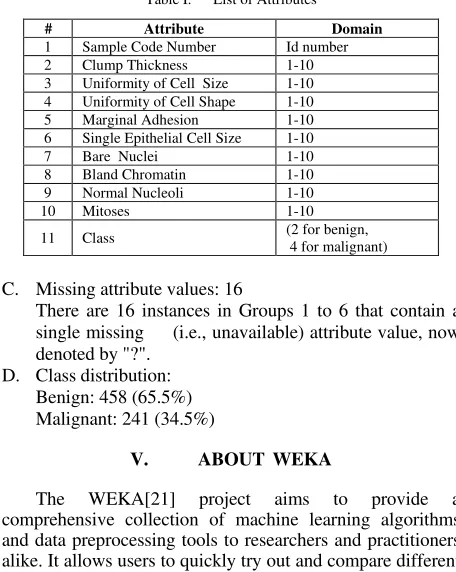
The investigation and elucidation of classification is a time overwhelming process that requires a deep perceptive of statistics. The result of Tables V, VI, VII and VIII shows that all the significant attributes shows approximately equal no of correct classification. Bayesnet Classifier outperforms

the remaining algorithms. It is observed that after performing feature reduction method Logistic has a significant improvement in their classification. The fig 2 depicts the performance of the classification methods after feature reduction.

Correctly classified instances of 6 Classification algorithms based on various attribute selection

86.00%

Figure 2. Correctly Classified instances of 6 classification algoirhtms after feature reduction

Incorrectly classified instances of 6 Classification algorithms based on various attribute selection

0.00%

Figure 3. InCorrectly Classified instances of 6 classification algoirhtms after feature reduction

XI. CONCLUSION

It is observed that the feature selection of potential attributes reduces the overall time of the classification algorithms. Bayes net classifier outperforms the remaining algorithms used in this paper. After reducing the attributes to 6, 5 and 4 using rank search, genetic search and greedy step wise search the performance of the classification algorithms are improved. It is noted that Logistic Classifiers performance is increased after Feature reduction.

XII. REFERENCES

[1] National Cancer Institute (June 27, 2005). "Paget's Disease of the Nipple: Questions and Answers".

http://www.cancer.gov/cancertopics/factsheet/Sites-Types/pagets-breast. Retrieved 2008-02-06.

[2] "Male Breast Cancer Treatment". National Cancer Institute. 2006. http://www.cancer.gov /cancertopics /pdq/treatment/malebreast/healthprofessional. Retrieved machine learning tools and techniques, 2nd Edition. San Fransisco:Morgan Kaufmann, 2005.

(7)

[7] Zhou ZH, Jiang Y. Medical diagnosis with C4.5 Rule preceded by artificial neural network ensemble. IEEE Trans Inf Technol Biomed. 2003 Mar; 7(1):37-42.

[8] Lundin M, Lundin J, Burke HB, Toikkanen S, Pylkkanen L, Joensuu H. Artificial neural networks applied to survival prediction in breast cancer. Oncology 1999; 57:281- 6.

[9] Delen D, Walker G, Kadam A. Predicting breast cancer survivability: a comparison of three data mining methods. Artificial Intelligence in Medicine. 2005 Jun; 34(2):113-27.

[10] G. Fort, S. Lambert Lacroix, “Classification using partial least squares with penalized logistic regression”, England: Bioinformatics-Oxford, 2005.

[11] S. Bicciato, A. Luchini, C. Di-Bello, “Marker identification and classification of cancer types using gene expression data and SIMCA”, Germany: Methods-of-information-in-medicine, 2004

[12] K. A. Marx, P. O'Neil, P. Hoffman, M. L. Ujwal, “Data mining the NCI cancer cell line compound GI(50) values: identifying quinone subtypes effective against melanoma and leukemia cell classes”, United-States: Journal-of-chemical-information-and-computer-sciences, 2003.

[13] O. L. Mangasarian and W. H. Wolberg: "Cancer diagnosis via linear programming", SIAM News, Volume 23, Number 5, September 1990, pp 1 & 18.

[14] William H. Wolberg and O.L. Mangasarian:

"Multisurface method of pattern separation for medical diagnosis applied to breast cytology", Proceedings of the National Academy of Sciences, U.S.A., Volume 87, December 1990, pp 9193-9196.

[15] O. L. Mangasarian, R. Setiono, and W.H. Wolberg: "Pattern recognition via linear programming: Theory and application to medical diagnosis", in: "Large-scale numerical optimization", Thomas F. Coleman and YuyingLi, editors, SIAM Publications, Philadelphia 1990, pp 22-30.

[16] K. P. Bennett & O. L. Mangasarian: "Robust linear programming discrimination of two linearly inseparable sets", Optimization Methods and Software 1, 1992, 23-34 (Gordon & Breach Science Publishers).

[17] C. Shearer. The CRISP-DM model: The new blueprint for data mining.Journal of Data Warehousing, 5(4), 2000.

[18] S.B. Kotsiantis, Supervised Machine Learning: A Review of Classification Techniques, Informatica 31(2007) 249-268, 2007

[19] Ultsch A (2003). U*-Matrix: a tool to visualize clusters in high dimentional data. University of Marburg, Department of Computer Science, Technical Report Nr. 36:1-12

[20] Yin H. Learning Nonlinear Principal Manifolds by Self-Organising Maps, In: Gorban A. N. et al. (Eds.), LNCSE 58, Springer, 2007 ISBN 978-3-540-73749-0

[21] WEKA: Data Mining Software in Java

(2008),http://www.cs.waikata.ac.nz/ml/weka

[22] Ben-Gal, Irad. "Bayesian Networks". In Ruggeri, Fabrizio; Kennett, Ron S.; Faltin, Frederick W. Encyclopedia of Statistics in Quality and Reliability.

John Wiley & Sons.

doi:10.1002/9780470061572.eqr089.ISBN 978-0-470-01861-3.

[23] Ross J. Quinlan: Learning with Continuous Classes. In: 5th Australian Joint Conference on Artificial Intelligence, Singapore, 343-348, 1992.

[24] Agresti A (2007). "Building and applying logistic regression models". An Introduction to Categorical Data Analysis. Hoboken, New Jersey: Wiley. p. 138. ISBN 978-0-471-22618-5.