Proceedings of the Workshop on Cognitive Aspects of Computational Language Acquisition, pages 81–88,
The Benefits of Errors:
Learning an OT Grammar with a Structured Candidate Set
Tam´as Bir´o
ACLC, Universiteit van Amsterdam Spuistraat 210
Amsterdam, The Netherlands [email protected]
Abstract
We compare three recent proposals adding a topology to OT: McCarthy’s Persistent OT, Smolensky’s ICS and B´ır´o’s SA-OT. To test their learnability, constraint rankings are learnt from SA-OT’s output. The errors in the output, being more than mere noise, fol-low from the topology. Thus, the learner has to reconstructs her competence having ac-cess only to the teacher’s performance.
1 Introduction: topology and OT
The year 2006 witnessed the publication of sev-eral novel approaches within Optimality Theory (OT) (Prince and Smolensky, 1993 aka 2004) intro-ducing some sort of neighbourhood structure (topol-ogy, geometry) on the candidate set. This idea has been already present since the beginnings of OT but its potentialities had never been really developed un-til recently. The present paper examines the learn-ability of such an enriched OT architecture.
Traditional Optimality Theory’s GEN function generates a huge candidate set from the underlying form (UF) and then EVAL finds the candidatewthat optimises the Harmony functionH(w)on this unre-stricted candidate set. H(w)is derived from the vi-olation marks assigned by a ranked set of constraints tow. The surface form SF corresponding to UF is the (globally) optimal element of GEN(UF):
SF(UF) =argoptw∈GEN(UF)H(w) (1)
Yet, already Prince and Smolensky (1993/2004:94-95) mention the possibility of
restricting GEN, creating an alternative closer to standard derivations. Based the iterative syllabifi-cation in Imdlawn Tashlhiyt Berber, they suggest: “some general procedure (Do-α) is allowed to make a certain single modification to the input, producing the candidate set of all possible outcomes of such modification.” The outputs of Do-α are “neighbours” of its input, so Do-α defines a topol-ogy. Subsequently, EVAL finds the most harmonic element of this restricted candidate set, which then serves again as the input of Do-α. Repeating this procedure again and again produces a sequence of neighbouring candidates with increasing Harmony, which converges toward the surface form.
Calling Do-αa restricted GEN, as opposed to the freedom of analysis offered by the traditional GEN, McCarthy (2006) develops this idea into the Per-sistent OT architecture (aka. harmonic serialism, cf. references in McCarthy 2006). He demonstrates on concrete examples how repeating the GEN → EVAL → GEN→ EVAL →... cycle until reach-ing some local optimum will produce a more restric-tive language typology that conforms rather well to observation. Importantly for our topic, learnabil-ity, he claims that Persistent OT “can impose stricter ranking requirements than classic OT because of the need to ensure harmonic improvement in the inter-mediate forms as well as the ultimate output ”.
In two very different approaches, both based on the traditional concept of GEN, Smolensky’s Inte-grated Connectionist/Symbolic (ICS) Cognitive Ar-chitecture (Smolensky and Legendre, 2006) and the strictly symbolic Simulated Annealing for Op-timality Theory Algorithm (SA-OT) proposed by
B´ır´o (2005a; 2005b; 2006a), use simulated anneal-ing to find the best candidate w in equation (1). Simulated annealing performs a random walk on the search space, moving to a similar (neighbouring) el-ement in each step. Hence, it requires a topology on the search space. In SA-OT this topology is directly introduced on the candidate set, based on a linguis-tically motivated symbolic representation. At the same time, connectionist OT makes small changes in the state of the network; so, to the extent that states correspond to candidates, we obtain again a neigh-bourhood relation on the candidate set.
Whoever introduces a neighbourhood structure (or a restricted GEN) also introduces local optima: candidates more harmonic than all their neighbours, independently of whether they are globally opti-mal. Importantly, each proposal is prone to be stuck in local optima. McCarthy’s model repeats the generation-evaluation cycle as long as the first local optimum is not reached; whereas simulated anneal-ing is a heuristic optimisation algorithm that some-times fails to find the global optimum and returns another local optimum. How do these proposals in-fluence the OT “philosophy”?
For McCarthy, the first local optimum reached from UF is the grammatical form (the surface form predicted by the linguistic competence model), so he rejects equation (1). Yet, Smolensky and B´ır´o keep the basic idea of OT as in (1), and B´ır´o (2005b; 2006a) shows the errors made by simulated anneal-ing can mimic performance errors (such as stress shift in fast speech). So mainstream Optimality Theory remains the model of linguistic competence, whereas its cognitively motivated, though imperfect implementation with simulated annealing becomes a model of linguistic performance. Or, as B´ır´o puts it, a model of the dynamic language production pro-cess in the brain. (See also Smolensky and Legen-dre (2006), vol. 1, pp. 227-229.)
In the present paper we test the learnability of an OT grammar enriched with a neighbourhood struc-ture. To be more precise, we focus on the latter ap-proaches: how can a learner acquire a grammar, that is, the constraint hierarchy defining the Harmony functionH(w), if the learning data are produced by a performance model prone to make errors? What is the consequence of seeing errors not simply as mere noise, but as the result of a specific mechanism?
2 Walking in the candidate set
First, we introduce the production algorithms (sec-tion 2) and a toy grammar (sec(sec-tion 3), before we can run the learning algorithms (section 4).
Equation (1) defines Optimality Theory as an op-timisation problem, but finding the optimal candi-date can be NP-hard (Eisner, 1997). Past solutions— chart parsing (Tesar and Smolensky, 2000; Kuhn, 2000) and finite state OT (see Biro (2006b) for an overview)—require conditions met by several, but not by all linguistic models. They are also “too per-fect”, not leaving room for performance errors and computationally too demanding, hence cognitively not plausible. Alternative approaches are heuris-tic optimization techniques: geneheuris-tic algorithms and simulated annealing.
These heuristic algorithms do not always find the (globally) optimal candidate, but are simple and still efficient because they exploit the structure of the candidate set. This structure is realized by a neigh-bourhood relation: for each candidatewthere exists a set Neighbours(w), the set of the neighbours of w. It is often supposed that neighbours differ only minimally, whatever this means. The neigh-bourhood relation is usually symmetric, irreflexive and results in a connected structure (any two candi-dates are connected by a finite chain of neighbours). The topology (neighbourhood structure) opens the possibility to a (random) walk on the candi-date set: a series w0, w1, w2, ..., wL such that for
all 0 ≤ i < L, candidate wi+1 is wi or a
neigh-bour ofwi. (Candidatew0 will be called winit, and
wL will bewfinal, henceforth.) Genetic algorithms
start with a random population of winit’s, and em-ploy OT’s EVAL function to reach a population of
wfinal’s dominated by the (globally) optimal candi-date(s) (Turkel, 1994). In what follows, however, we focus on algorithms using a single walk only.
The simplest algorithm, gradient descent, comes in two flavours. The version on Fig. 1 defineswi+1
as the best element of set{wi}∪Neighbours(wi).
It runs as long aswi+1differs fromwi, and is
ALGORITHM Gradient Descent: OT with restricted GEN w := w_init;
repeat
w_prev := w;
w := most_harmonic_element( {w_prev} U Neighbours(w_prev) );
until w = w_prev
return w # w is an approximation to the optimal solution
Figure 1: Gradient Descent: iterated Optimality Theory with a restricted GEN (Do-α).
ALGORITHM Randomized Gradient Descent w := w_init ;
repeat
Randomly select w’ from the set Neighbours(w);
if (w’ not less harmonic than w) then w := w’;
until stopping condition = true
return w # w is an approximation to the optimal solution
Figure 2: Randomized Gradient Descent
The second version of gradient descent is stochastic (Figure 2). In step i, a ran-dom w′
∈ Neighbours(wi) is chosen
us-ing some pre-defined probability distribution on Neighbours(wi) (often a constant function). If
neighbourw′ is not worse thanw
i, then the next
el-ement wi+1 of the random walk will be w′;
other-wise, wi+1 is wi. The stopping condition requires
the number of iterations reach some value, or the average improvement of the target function in the last few steps drop below a threshold. The output is
wfinal, a local optimum if the walk is long enough. Simulated annealing (Fig. 3) plays with this sec-ond theme to increase the chance of finding the global optimum and avoid unwanted local optima. The idea is the same, but ifw′
is worse thanwi, then
there is still a chance to move tow′. The transition probability of moving to w′ depends on the target function E atwi and w′, and on ‘temperature’ T:
P(wi → w′|T) = exp
−E(w′)−E(wi)
T
. Using a randomr, we move tow′ iff r < P(w
i → w′|T).
TemperatureT is gradually decreased following the cooling schedule. Initially the system easily climbs larger hills, but later it can only descend valleys. Im-portantly, the probability wfinal is globally optimal converges to1as the number of iterations grows.
But the target function is not real-valued in Op-timality Theory, so how can we calculate the tran-sition probability? ICS (Smolensky and Legendre, 2006) approximates OT’s harmony function with a real-valued target function, while B´ır´o (2006a)
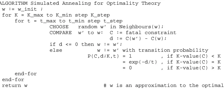
in-troduces a novel algorithm (SA-OT, Figure 4) to guarantee the principle of strict domination in the constraint ranking. The latter stays on the purely symbolic level familiar to the linguist, but does not always display the convergence property of tradi-tional simulated annealing.
Temperature in the SA-OT Algorithm is a pair
(K, t) with t > 0, and is diminished in two, em-bedded loops. Similarly, the difference in the target function (Harmony) is not a single real number but a pair(C, d). HereCis the fatal constraint, the high-est ranked constraint by whichwiandw′behave
dif-ferently, whiledis the difference of the violations of this constraint. (ForH(wi) = H(w′)let the
differ-ence be(0,0).) Each constraint is assigned a real-valued rank (most often an integer; we shall call it a K-value) such that a higher ranked constraint has a higher K-value than a lower ranked constraint (hi-erarchies are fully ranked). The K-value of the fatal constraint corresponds to the first component of the temperature, and the second component of the dif-ference in the target function corresponds to the sec-ond component of the temperature. The transition probability fromwi to its neighbourw′ is1ifw′ is
not less harmonic thanwi; otherwise, the originally
exponential transition probability becomes
P wi→w′|(K, t)
=
1 if K-value of C< K e−d
t if K-value of C=K
ALGORITHM Simulated Annealing
w := w_init ; T := T_max ;
repeat
CHOOSE random w’ in Neighbours(w);
Delta := E(w’) - E(w);
if ( Delta < 0 ) then w := w’;
else # move to w’ with transition probability P(Delta;T) = exp(-Delta/T):
generate random r uniformly in range (0,1);
if ( r < exp(-Delta / T) ) then w := w’;
T := alpha(T); # decrease T according to some cooling schedule
until stopping condition = true
return w # w is an approximation to the minimal solution
Figure 3: Minimizing a real-valued energy functionE(w)with simulated annealing.
Again,wi+1isw′if the random numberrgenerated
between 0 and 1 is less than this transition proba-bility; otherwise wi+1 = wi. B´ır´o (2006a, Chapt.
2-3) argues that this definition fits best the underly-ing idea behind both OT and simulated annealunderly-ing.
In the next part of the paper we focus on SA-OT, and return to the other algorithms afterwards only.
3 A string grammar
To experiment with, we now introduce an abstract grammar that mimics real phonological ones.
Let the set of candidates generated by GEN for any input be{0,1, ..., P −1}L
, the set of strings of lengthLover an alphabet ofP phonemes. We shall use L = P = 4. Candidate w′ is a neighbour of candidate w if and only if a single minimal oper-ation (a basic step) transforms w into w′
. A min-imal operation naturally fitting the structure of the candidates is to change one phoneme only. In or-der to obtain a more interesting search space and in order to meet some general principles—the neigh-bourhood relation should be symmetric, yielding a connected graph but be minimal—a basic step can only change the value of a phoneme by1moduloP. For instance, in theL =P = 4case, neighbours of
0123are among others1123,3123,0133and0120, but not1223,2123or0323. If the four phonemes are represented as a pair of binary features (0 = [−−],
1 = [+−],2 = [++]and3 = [−+]), then this basic step alters exactly one feature.
We also need constraints. Constraint No-ncounts the occurrences of phoneme n (0 ≤ n < P) in the candidate (i.e., assigns one violation mark per phoneme n). Constraint No-initial-n punishes phonemenword initially only, whereas No-final-n
does the same word finally. Two more constraints sum up the number of dissimilar and similar pairs of adjacent phonemes. Letw(i) be theith phoneme in
stringw, and let[b] = 1ifbis true and[b] = 0ifbis false; then we have3P + 2markedness constraints:
No-n: non(w) =PL−1
i=0[w(i)=n]
No-initial-n: nin(w) = [w(0)=n]
No-final-n: nfn(w) = [w(L−1) =n] Assimilate: ass(w) =PL−2
i=0[w(i)6=w(i+1)]
Dissimilate: dis(w) =PL−2
i=0[w(i)=w(i+1)]
Grammars also include faithfulness constraints punishing divergences from a reference string σ, usually the input. Ours sums up the distance of the phonemes inwfrom the corresponding ones inσ:
FAITHσ(w) =P L−1
i=0 d(σ(i), w(i))
where d(a, b) = min((a − b) modP,(b − a) mod P))is the minimal number of basic steps trans-forming phonemeaintob. In our case, faithfulness is also the number of differing binary features.
To illustrate SA-OT, we shall use grammarH:
H: no0 ≫ ass≫ Faithσ=0000 ≫ ni1 ≫
ni0≫ni2≫ni3≫nf0≫nf1≫nf2≫ nf3≫no3≫no2≫no1≫dis
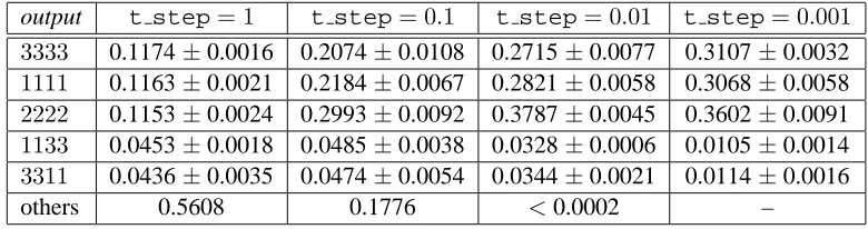
A quick check proves that the global optimum is candidate 3333, but there are many other local optima: 1111, 2222, 3311, 1333, etc. Table 1 shows the frequencies of the outputs as a function oft step, all other parameters kept unchanged.
Several characteristics of SA-OT can be observed. For hight step, the thirteen local optima ({1,3}4
ALGORITHM Simulated Annealing for Optimality Theory w := w_init ;
for K = K_max to K_min step K_step for t = t_max to t_min step t_step
CHOOSE random w’ in Neighbours(w);
COMPARE w’ to w: C := fatal constraint
d := C(w’) - C(w); if d <= 0 then w := w’;
else w := w’ with transition probability
P(C,d;K,t) = 1 , if K-value(C) < K
= exp(-d/t) , if K-value(C) = K
= 0 , if K-value(C) > K
end-for end-for
[image:5.612.74.454.70.221.2]return w # w is an approximation to the optimal solution
Figure 4: The Simulated Annealing for Optimality Theory Algorithm (SA-OT).
iterations increases (parameter t step drops), the probability of finding the globally optimal candidate grows. In many grammars (e.g., ni1 and ni3 moved to between no0 and ass inH), the global optimum is the only output for smallt stepvalues. Yet,H also yields irregular forms: 1111 and 2222 are not globally optimal but their frequencies grow together with the frequency of3333.
4 Learning grammar from performance
To summarise, given a grammar, that is, a constraint hierarchy, the SA-OT Algorithm produces perfor-mance forms, including the grammatical one (the global optimum), but possibly also irregular forms and performance errors. The exact distribution de-pends on the parameters of the algorithm, which are not part of the grammar, but related to external (physical, biological, pragmatic or sociolinguistic) factors, for instance, to speech rate.
Our task of learning a grammar can be formulated thus: given the output distribution of SA-OT based on the target OT hierarchy (the target grammar), the learner seeks a hierarchy that produces a simi-lar performance distribution using the same SA-OT Algorithm. (See Yang (2002) on grammar learning as parameter setting in general.) Without any infor-mation on grammaticality, her goal is not to mimic competence, not to find a hierarchy with the same global optima. The grammar learnt can diverge from the target hierarchy, as long as their performance is comparable (see also Apoussidou (2007), p. 203). For instance, if ni1 and ni3 change place in gram-marH, the grammaticality of1111and3333are
versed, but the performance stays the same. This re-sembles two native speakers whose divergent gram-mars are revealed only when they judge differently forms otherwise produced by both.
We suppose that the learner employs the same SA-OT parameter setting. The acquisition of the parameters is deferred to future work, because this task is not part of language acquisition but of social acculturation: given a grammar, how can one learn which situation requires what speed rate or what level of care in production? Consequently, fine-tuning the output frequencies, which can be done by fine-tuning the parameters (such ast step) and not the grammar, is not our goal here. But language learners do not seem to do it, either.
Learning algorithms in Optimality Theory belong to two families: off-line and on-line algorithms. Off-line algorithms, the prototype of which is Recur-sive Constraint Demotion (RCD) (Tesar, 1995; Tesar and Smolensky, 2000), first collect the data and then attempt to build a hierarchy consistent with them. On-line algorithms, such as Error Driven Constraint Demotion (ECDC) (Tesar, 1995; Tesar and Smolen-sky, 2000) and Gradual Learning Algorithm (GLA) (Boersma, 1997; Boersma and Hayes, 2001), start with an initial hierarchy and gradually alter it based on discrepancies between the learning data and the data produced by the learner’s current hierarchy.
output t step= 1 t step= 0.1 t step= 0.01 t step= 0.001 3333 0.1174±0.0016 0.2074±0.0108 0.2715±0.0077 0.3107±0.0032
1111 0.1163±0.0021 0.2184±0.0067 0.2821±0.0058 0.3068±0.0058
2222 0.1153±0.0024 0.2993±0.0092 0.3787±0.0045 0.3602±0.0091
1133 0.0453±0.0018 0.0485±0.0038 0.0328±0.0006 0.0105±0.0014
3311 0.0436±0.0035 0.0474±0.0054 0.0344±0.0021 0.0114±0.0016
[image:6.612.110.500.71.174.2]others 0.5608 0.1776 <0.0002 –
Table 1: Outputs of SA-OT for hierarchyH. “Others” are twelve forms, each with a frequency between 2% and 8% fort step= 1, and lower than 4.5% fort step= 0.1. (Forms produced in 8% of the cases at t step= 1are not produced ift step= 0.01!) An experiment consisted of running 4096 simulations and counting relative frequencies; each cell contains the mean and standard deviation of three experiments.
development. (Although on-line algorithms require virtual production only, not necessarily uttered in communication, we suppose the two go together.) We defer for future work issues as parsing hidden structures, learning underlying forms and biases for ranking markedness above faithfulness.
4.1 Learning SA-OT
We first implemented Recursive Constraint Demo-tion with SA-OT. To begin with, RCD creates a win-ner/loser table, in which rows correspond to pairs
(w, l) such that winnerw is a learning datum, and loser l is less harmonic than w. Column winner marks contains the constraints that are more severely violated by the winner than by the loser, and vice-versa for column loser marks. Subsequently, RCD builds the hierarchy from top. It repeatedly collects the constraints not yet ranked that do not occur as winner marks. If no such constraint exists, then the learning data are inconsistent. These constraints are then added to the next stratum of the hierarchy in a random order, while the rows in the table containing them as loser marks are deleted (because these rows have been accounted for by the hierarchy).
Given the complexity of the learning data pro-duced by SA-OT, it is an advantage of RCD that it recognises inconsistent data. But how to collect the winner-loser pairs for the table? The learner has no information concerning the grammaticality of the learning data, and only knows that the forms pro-duced are local optima for the target (unknown) hi-erarchy and the universal (hence, known) topology. Thus, we constructed the winner-loser table from all pairs(w, l)such that wwas an observed form, and
lwas a neighbour ofw. To avoid the noise present in real-life data, we considered onlyw’s with a fre-quency higher than√N, where N was the number of learning data. Applying then RCD resulted in a hierarchy that produced the observed local optima— and most often also many others, depending on the random constraint ranking in a stratum. These un-wanted local optima suggest a new explanation of some “child speech forms”.
Therefore, more information is necessary to find the target hierarchy. As learners do not use nega-tive evidence (Pinker, 1984), we did not try to re-move extra local optima directly. Yet, the learners do collect statistical information. Accordingly, we en-riched the winner/loser table with pairs(w, l) such that wwas a form observed significantly more fre-quently thanl;l’s were observed forms and the extra local optima. (A difference in frequency was signifi-cant if it was higher than√N.) The assumption that frequency reflects harmony is based on the heuris-tics of SA-OT, but is far not always true. So RCD recognised this new table often to be inconsistent.
Enriching the table could also be done gradually, adding a new pair only if enough errors have sup-ported it (Error-Selective Learning, Tessier (2007). The pair is then removed if it proves inconsistent with stronger pairs (pairs supported by more errors, or pairs of observed forms and their neighbours).
reranking two constraints. The GLA Algorithm as-signs a real-valued rankrto each constraint, so that a higher ranked constraint has a higherr. Then, in each learning step the learning datum (the winner) is compared to the output produced by the learner’s actual hierarchy (the loser). Every constraint’s rank is decreased by a small value (the plasticity) if the winner violates it more than the loser, and it is in-creased by the same value if the loser has more vi-olations than the winner. Often—still, not always (Pater, 2005)—these small steps accumulate to con-verge towards the correct constraint ranking.
When producing an output (the winner) for the target hierarchy and another one (the loser) for the learner’s hierarchy, Boersma uses Stochastic OT (Boersma, 1997). But one can also employ tradi-tional OT evaluation, whereas we used SA-OT with t step = 0.1. The learner’s actual hierarchy in GLA is stored by the real-valued ranks r. So the fatal constraint in the core of SA-OT (Fig. 4) is the constraint that has the highestr among the con-straints assigning different violations to w and w′. (A random one of them, if more constraints have the same r-values, but this is very rare.). The K-values were the floor of the r-values. (Note the possibil-ity of more constraints having the same K-value.) The r-values could also be directly the K-values; but since parametersK max,K minandK stepare in-tegers, this would cause the temperature not enter the domains of the constraints, which would skip an important part of simulated annealing.
Similarly to Stochastic OT, our model also dis-played different convergence properties of GLA. Quite often, GLA reranked its initial hierarchy (the output of RCD) into a hierarchy yielding the same or a similar output distribution to that produced by the target hierarchy. The simulated child’s perfor-mance converged towards the parent’s perforperfor-mance, and “child speech forms” were dropped gradually.
In other cases, however, the GLA algorithm turned the performance worse. The reason for that might be more than the fact that GLA does not al-ways converge. Increasing or decreasing the con-straints’ rank by a plasticity in GLA is done in or-der to make the winners gradually better and the losers worse. But in SA-OT the learner’s hierarchy can produce a form that is indeed more harmonic (but not a local optimum) for the target ranking than
the learning datum; then the constraint promotions and demotions miss the point. Moreover, unlike in Stochastic OT, these misguided moves might be more frequent than the opposite moves.
Still, the system performed well with our gram-mar H. Although the initial grammars returned by RCD included local optima (“child speech forms”, e.g.,0000), learning with GLA brought the learner’s performance most often closer to the teacher’s. Still, final hierarchies could be very diverse, with different global optima and frequency distributions.
In another experiment the initial ranking was the target hierarchy. Then, 13 runs returned the target distribution with some small changes in the hierar-chy; in five cases the frequencies changed slightly, but twice the distribution became qualitatively dif-ferent (e.g.,2222not appearing).
4.2 Learning in other architectures
Learning in the ICS architecture involves similar problems to those encountered with SA-OT. The learner is faced again with performance forms that are local optima and not always better than unat-tested forms. The learning differs exclusively as a consequence of the connectionist implementation.
In McCarthy’s Persistent OT, the learner only knows that the observed form is a local optimum, i. e., it is better than all its neighbours. Then, she has to find a path backwards, from the surface form to the underlying form, such that in each step the can-didate closer to the SF is better than all other neigh-bours of the candidate closer to the UF. Hence, the problem is more complex, but it results in a similar winner/loser table of locally close candidates.
5 Conclusion and future work
the fact that different parameter settings of SA-OT yield different distributions.
Not correctly reconstructed grammars often lead to different grammaticality judgements, but also to quantitative differences in the performance distribu-tion, despite the qualitative similarity. This fact can explain diachronic changes and why some grammars are evolutionarily more stable than others.
Inaccurate reconstruction, as opposed to exact learning, is similar to what Dan Sperber and oth-ers said about symbolic-cultural systems: “The tacit knowledge of a participant in a symbolic-cultural system is neither taught nor learned by rote. Rather each new participant [...] reconstructs the rules which govern the symbolic-cultural system in ques-tion. These reconstructions may differ considerably, depending upon such factors as the personal his-tory of the individual in question. Consequently, the products of each individual’s symbolic mechanism are idiosyncratic to some extent.” (Lawson and Mc-Cauley, 1990, p. 68, italics are original). This obser-vation has been used to argue that cultural learning is different from language learning; now we turn the table and claim that acquiring a language is indeed similar in this respect to learning a culture.
References
Diana Apoussidou. 2007. The Learnability of Metrical Phonology. Ph.D. thesis, University of Amsterdam.
Tam´as B´ır´o. 2005a. How to define Simulated Annealing
for Optimality Theory? In Proc. 10th FG and 9th
MoL, Edinburgh. Also ROA-8971.
Tam´as B´ır´o. 2005b. When the hothead speaks: Sim-ulated Annealing Optimality Theory for Dutch fast speech. In C. Cremers et al., editor, Proc. of the 15th CLIN, pages 13–28, Leiden. Also ROA-898.
Tam´as B´ır´o. 2006a. Finding the Right Words: Imple-menting Optimality Theory with Simulated Annealing. Ph.D. thesis, University of Groningen. ROA-896.
Tam´as B´ır´o. 2006b. Squeezing the infinite into the fi-nite. In A. Yli-Jyr et al., editor, Finite-State Methods and Natural Language Processing, FSMNLP 2005, Helsinki, LNAI-4002, pages 21–31. Springer.
Paul Boersma and Bruce Hayes. 2001. Empirical tests of the Gradual Learning Algorithm. Linguistic Inquiry, 32:45–86. Also: ROA-348.
1
ROA: Rutgers Optimality Archive at http://roa.rutgers.edu
Paul Boersma. 1997. How we learn variation, option-ality, and probability. Proceedings of the Institute of Phonetic Sciences, Amsterdam (IFA), 21:43–58.
Jason Eisner. 1997. Efficient generation in primitive op-timality theory. In Proc. of the 35th Annual Meeting of the Association for Computational Linguistics and 8th EACL, pages 313–320, Madrid.
Judit Gervain, Marina Nespor, Reiko Mazuka, Ryota Horie, and Jacques Mehler. submitted. Bootstrapping word order in prelexical infants: a japanese-italian cross-linguistic study. Cognitive Psychology.
Jonas Kuhn. 2000. Processing optimality-theoretic syn-tax by interleaved chart parsing and generation. In Proc.ACL-38, Hongkong, pages 360–367.
E. Thomas Lawson and Robert N. McCauley. 1990. Re-thinking Religion: Connecting Cognition and Culture. Cambridge University Press, Cambridge, UK.
John J. McCarthy. 2006. Restraint of analysis. In
E. Bakovi´c et al., editor, Wondering at the Natural Fe-cundity of Things: Essays in Honor of A. Prince, pages 195–219. U. of California, Santa Cruz. ROA-844.
Joe Pater. 2005. Non-convergence in the GLA and vari-ation in the CDA. ms., ROA-780.
Steven Pinker. 1984. Language Learnability & Lan-guage Development. Harvard UP, Cambridge, Mass.
Alan Prince and Paul Smolensky. 1993 aka 2004.
Optimality Theory: Constraint Interaction in Gen-erative Grammar. Blackwell, Malden, MA, etc. Also: RuCCS-TR-2, 1993; ROA Version: 537-0802, http://roa.rutgers.edu, 2002.
Jenny R. Saffran, Richard N. Aslin, and Elissa L. New-port. 1996. Statistical learning by 8-month-old in-fants. Science, 274(5294):1926–1928.
Paul Smolensky and G´eraldine Legendre. 2006.
The Harmonic Mind: From Neural Computation to Optimality-Theoretic Grammar. MIT P., Cambridge.
Bruce Tesar and Paul Smolensky. 2000. Learnability in Optimality Theory. MIT Press, Cambridge, MA.
Bruce Tesar. 1995. Computational Optimality Theory. Ph.D. thesis, University of Colorado. Also: ROA-90.
Anne-Michelle Tessier. 2007. Biases and Stages in
Phonological Acquisition. Ph.D. thesis, University of Massachusetts Amherst. Also: ROA-883.
Bill Turkel. 1994. The acquisition of Optimality Theo-retic systems. m.s., ROA-11.