Comparative Analysis to Highlight Pros and Cons
of Data Mining Techniques-Clustering, Neural
Network and Decision Tree
Aarti Kaushal , Manshi Shukla
Assistant Professor, Computer Science and Engineering, RIMT- Institute of Engineering and Technology,
Near Floating Restaurant, Ambala-Ludhiana NH-1, Sirhind Side, Mandi Godindgarh-147301, Panjab, India
Abstract- In the current competitive world, we require an efficient technique to summarize, analyse, present and maintain large datasets using data mining. This requires the knowledge of all data mining techniques in order to choose the best for desired datasets and these data mining techniques can answer business questions that traditionally were too time consuming to resolve. They scour databases for hidden patterns, finding predictive information that experts may miss because it lies outside their expectations. Considering this, in this paper we provide an introduction to the basic technologies of data mining. The concept is illustrated with examples that incorporate real dataset of different cities in India. We explore and compare three data mining techniques- clustering, neural network and decision trees with an introduction on the general concepts of data mining and these techniques. The comparison among the three techniques is exhibited with their favourable and adverse effects.
Keyword- Data Mining, Clustering, Neural Network, Decision Tree, Comparison.
I. INTRODUCTION
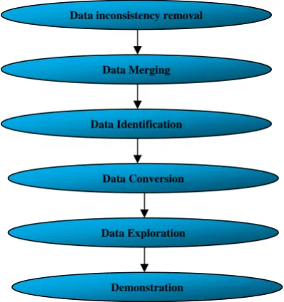
Data Mining is the withdrawal of knowledge from tremendously large datasets, detection of the non apparent facts that can perk up data analysis, interpretation and prediction process. Data mining is an automated discovery process of nontrivial, previously unknown and potentially useful patterns embedded in databases (e.g. [23]). It is the technology that enables data exploration and data visualisation of very huge databases at a high level of abstraction which requires no specific hypothesis in mind. This extraction of hidden predictive information from large datasets has great potential to help companies to focus on the most significant information in their data warehouses. Data mining is a process of following 7 D’s iterative sequence of steps (e.g. Fig. 1):
i. Data inconsistency removal ii. Data merging
iii. Data identification iv. Data conversion
v. Data exploration vi. Data configuration vii. Demonstration
Fig. 1 7 D’s of data mining process
Data mining as a term used for the specific set of 6 activities or tasks as follows:
cataloguing
evaluation
calculation
association rule
clustering
visualization
The first three tasks are the example of directed data mining or supervised learning. In this the goal is to use the available data to build a model that describes 1 or more particular attribute. The next 3 tasks are the examples of in directed data mining or unsupervised learning i.e, no attribute is singled out as a target; the goal is to establish a relationship among all the attributes.
Today data mining facilitates business with numerous approaches in order to systemise the process and explore the data in search for consistent patterns and then to formalize the findings by applying 7 D’s steps.
In this paper, we compare and analyse data mining techniques-clustering, neural network and decision tree to highlight pros and cons in a systematic approach. Our goal is to give the brief comparison between the above three techniques have been explored findings.
Data inconsistency removal
Data Merging
Data Identification
Data Conversion
Data Exploration
II. BACKGROUND
Research has shown that, data doubles every three years (e.g. [24]).Thus data mining has become an important tool to transform these data into information.
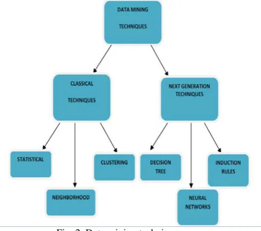
These techniques (e.g. Fig. 2) can be broken into two sections, each with a specific theme:
Classical Techniques: Statistics, Neighborhoods and Clustering
Next Generation Techniques: Decision Trees, Neural Networks and Induction Rules
a) Statistics
Statistics is the study of the collection, organization, analysis, interpretation and presentation of data (e.g. [10]) . It deals with all aspects of data, including the planning of data collection in terms of the design of surveys and experiments (e.g. [10]). Statistical techniques focus on data and are used to discover patterns and models.
b) Neighbourhoods
Nearest neighbour is a prediction technique that is quite similar to clustering - its essence is that in order to predict what a prediction value is in one record look for records with similar predictor values in the historical database and use the prediction value from the record that it “nearest” to the unclassified record (e.g. [1]).
c) Clustering
Clustering is a process of dividing the set of data into a set of subclasses by which like records are grouped together.It can be used either as a stand-alone tool or as a preprocessing step.This provides high level view of data extraction.
d) Decision trees
A decision tree is a predictive model that is expressed as a recursive partition of the instance space, as its name implies, can be viewed as a tree. Specifically each branch of the tree is a classification question and the leaves of the tree are partitions of the dataset with their classification (e.g. [4]).
e) Neural network
Neural network is a learning process used for pattern recognition or data categorization .It is related with the neurons in the biological systems.
f) Rule induction
Rule induction is the most important technique of data mining and most common form of knowledge discovery in unsupervised learning systems because regularities hidden in data can frequently be expressed in terms of rules.Usually rules are expressions of the form
if (attribute−1; value −1) and (attribute−2; value −2) and and (attribute−n; value−n) then (decision; value) Some rule induction systems induce more complex rules, in which values of attributes may be expressed by negation of some values or by a value subset of the attribute domain (e.g. [2]).
In this paper, three techniques of Data Mining -clustering, neural network and decision trees are compared to find their advantages and disadvantages. The concept of all these techniques is explained in the paper with suitable examples.
III. CONCEPT OF THREE TECHNIQUES IN DATA
MINING –CLUSTERING,NEURAL
NETWORKS AND DECISION TREES
The actual data mining task is to automate analysis of large datasets to extract information required in the form of groups of data records. The datasets in data mining applications are often large and so new techniques are developed frequently and are being developed to deal with millions of objects having perhaps dozens or even hundreds of attributes. Hence classifying these datasets becomes an important problem in data mining (e.g. [25]). So, few techniques those can be used are statistics, clustering, neighbourhood, neural network, decision tree, rule induction or others. In order to identify the differences among three chosen techniques, their basic concept is discussed in this section.
Fig. 2 Data mining techniques
A. Clustering
similar data points (e.g. [20]). In this paper, hierarchical clustering methods are explained.
1) Hierarchical clustering: There are 2 types Hierarchical clustering: Agglomerative (bottom up) and Divisive (top down).In the first clustering methods we start with singleton object and recursively add two or more appropriate clusters and then stop when n number of clusters is achieved. In the second method we start with a big cluster and recursively divide into smaller clusters till n number of clusters is achieved.
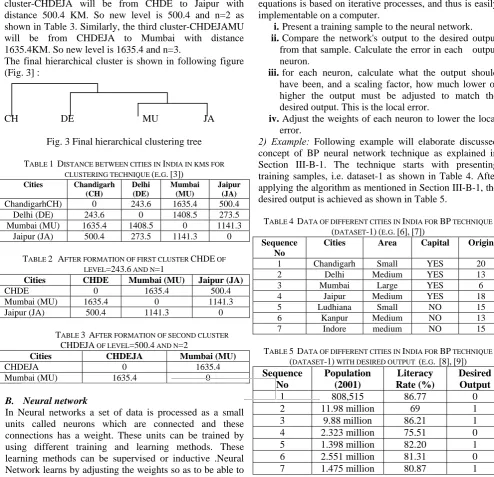
2) Example: Following example will elaborate discussed concept of clustering as discussed in Section III-A-1. The clustering starts with the formation of nearest pair of the cities as shown in Table 1. The first nearest pair of cities is Chandigarh and Delhi, at distance 243.6KM. These are merged into a single cluster called "CHDE". The new cluster has level 243.6 and sequence number, n=1 as shown in Table 2. Now in this paper we computed the distance from this new cluster to all other clusters. The second cluster-CHDEJA will be from CHDE to Jaipur with distance 500.4 KM. So new level is 500.4 and n=2 as shown in Table 3. Similarly, the third cluster-CHDEJAMU will be from CHDEJA to Mumbai with distance 1635.4KM. So new level is 1635.4 and n=3.
The final hierarchical cluster is shown in following figure (Fig. 3] :
CH DE MU JA
Fig. 3 Final hierarchical clustering tree
TABLE 1 DISTANCE BETWEEN CITIES IN INDIA IN KMS FOR CLUSTERING TECHNIQUE (E.G.[3])
Cities Chandigarh (CH)
Delhi (DE)
Mumbai (MU)
Jaipur (JA)
ChandigarhCH) 0 243.6 1635.4 500.4
Delhi (DE) 243.6 0 1408.5 273.5
Mumbai (MU) 1635.4 1408.5 0 1141.3
Jaipur (JA) 500.4 273.5 1141.3 0
TABLE 2 AFTER FORMATION OF FIRST CLUSTER CHDE OF LEVEL=243.6 AND N=1
Cities CHDE Mumbai (MU) Jaipur (JA)
CHDE 0 1635.4 500.4
Mumbai (MU) 1635.4 0 1141.3
Jaipur (JA) 500.4 1141.3 0
TABLE 3 AFTER FORMATION OF SECOND CLUSTER
CHDEJA OF LEVEL=500.4 AND N=2
Cities CHDEJA Mumbai (MU)
CHDEJA 0 1635.4
Mumbai (MU) 1635.4 0
B. Neural network
In Neural networks a set of data is processed as a small units called neurons which are connected and these connections has a weight. These units can be trained by using different training and learning methods. These learning methods can be supervised or inductive .Neural Network learns by adjusting the weights so as to be able to
correctly classify the training data and hence, after testing phase, to classify unknown data. Following Neural network techniques are used in data mining:
For Classification LVQ, and Kohonen are used
For Forecasting/Prediction BP, GRNN, and RBF are used
For pattern detection Recurrent Neural Networks are used
A complex system may be decomposed into simpler elements, in order to be able to understand it. Also simple elements may be gathered to produce a complex system (e.g. [21]). Thus, neural networks are mainly used for complex queries. Inspired by biological neural networks, ANNs are massively parallel computing systems consisting of an extremely large number of simple processors with many interconnections (e.g. [22]).
1) Back propagation neural network technique: The back propagation algorithm (e.g. [5]) is an involved mathematical tool; however, execution of the training equations is based on iterative processes, and thus is easily implementable on a computer.
i. Present a training sample to the neural network. ii. Compare the network's output to the desired output
from that sample. Calculate the error in each output neuron.
iii. for each neuron, calculate what the output should have been, and a scaling factor, how much lower or higher the output must be adjusted to match the desired output. This is the local error.
iv. Adjust the weights of each neuron to lower the local error.
2) Example: Following example will elaborate discussed concept of BP neural network technique as explained in Section III-B-1. The technique starts with presenting training samples, i.e. dataset-1 as shown in Table 4. After applying the algorithm as mentioned in Section III-B-1, the desired output is achieved as shown in Table 5.
TABLE 4 DATA OF DIFFERENT CITIES IN INDIA FOR BP TECHNIQUE (DATASET-1)(E.G.[6],[7])
Sequence No
Cities Area Capital Origin
1 Chandigarh Small YES 20
2 Delhi Medium YES 13
3 Mumbai Large YES 6
4 Jaipur Medium YES 18
5 Ludhiana Small NO 15
6 Kanpur Medium NO 13
7 Indore medium NO 15
TABLE 5 DATA OF DIFFERENT CITIES IN INDIA FOR BP TECHNIQUE (DATASET-1) WITH DESIRED OUTPUT (E.G. [8],[9]) Sequence
No
Population (2001)
Literacy Rate (%)
Desired Output
1 808,515 86.77 0
2 11.98 million 69 1
3 9.88 million 86.21 1
4 2.323 million 75.51 0
5 1.398 million 82.20 1
6 2.551 million 81.31 0
C. Decision tree
In data mining decision tree is used to describe the data and provides a tree that is used for decision making. Compared to other data-mining techniques, it is widely applied in various areas since it is robust to data scales or distributions (e.g. [27], [28]). They are easily understandable. Decision tree provides a modelling technique that is easy for humans to comprehend and is simplifies the classification process [26]. They only work over a single table, and over a single attribute at a time. Decision trees used in data mining are of two main types:
Classification tree
Regression tree
Decision tree algorithm recursively partitions a data set of records using depth-fist greedy approach (e.g. [29]) or breadth-first approach, until all the data items belong to a particular class are identified. The decision tree is formed in two phases: tree growing and tree pruning. The tree always grows in top-down format. In the tree pruning phase the full grown tree is cut back to prevent over fitting and improve the accuracy of the tree (e.g. [30]) in bottom up fashion. The tree pruning is important for decision tree formation. It is used to improve the prediction and
classification accuracy of the algorithm by minimizing the over-fitting (noise or much data in training data set) (e.g. [31]).
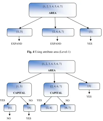
1) Example: Following example will elaborate the concept of decision tree as discussed in Section C. The process starts with the formation of tree for attribute area (e.g. Fig. 4, then for attribute capital (e.g. Fig. 5) and origin (e.g. Fig. 6), in order to achieve target as shown in Table 6. The range of area (in KM2) taken is as below:
Area <=400 is small, between 400 and 700 is medium and greater than 700 is larger
TABLE 6 DATA OF DIFFERENT CITIES IN INDIA FOR DECISION TREE TECHNIQUE (E.G.[6],[7])
S.
No Cities Area Capital Origin
Metropolitan City (Target)
1 Chandigarh Small YES 20 NO
2 Delhi Medium YES 13 YES
3 Mumbai Large YES 6 YES
4 Jaipur Medium YES 18 NO
5 Ludhiana Small NO 15 YES
6 Kanpur Medium NO 13 NO
7 Indore medium NO 15 YES
Fig. 4 Using attribute area (Level-1)
Fig. 5 Using attribute capital (Level-2) {1, 2, 3, 4, 5, 6, 7}
AREA
{3}
YES
{1, 5}
CAPITAL
{1}
YES NO
{5}
{2, 4, 6, 7}
CAPITAL
{2, 4}
YES NO
{6, 7}
YES
NO
{1, 2, 3, 4, 5, 6, 7}
AREA
{1, 5} {2, 4, 6, 7} {3}
YES
EXPAND
Fig. 6 Final decision tree after using attribute origin at Level-3
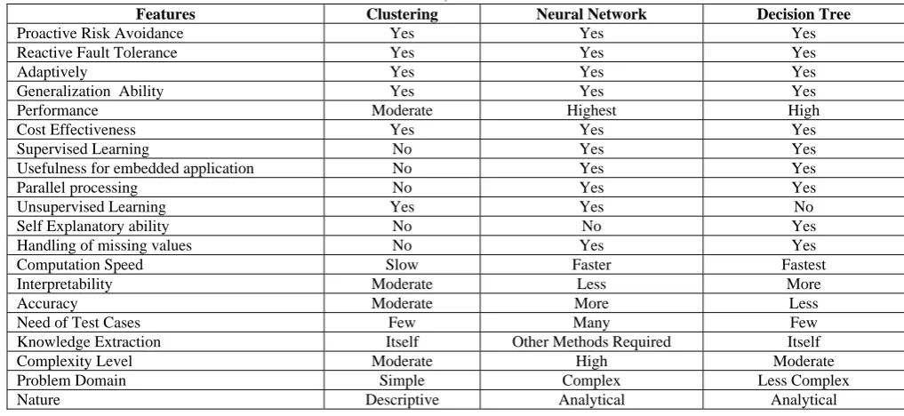
TABLE 7 FEATURES OF CLUSTERING, NEURAL NETWORK AND DECISION TREE
Features Clustering Neural Network Decision Tree
Proactive Risk Avoidance Yes Yes Yes
Reactive Fault Tolerance Yes Yes Yes
Adaptively Yes Yes Yes
Generalization Ability Yes Yes Yes
Performance Moderate Highest High
Cost Effectiveness Yes Yes Yes
Supervised Learning No Yes Yes
Usefulness for embedded application No Yes Yes
Parallel processing No Yes Yes
Unsupervised Learning Yes Yes No
Self Explanatory ability No No Yes
Handling of missing values No Yes Yes
Computation Speed Slow Faster Fastest
Interpretability Moderate Less More
Accuracy Moderate More Less
Need of Test Cases Few Many Few
Knowledge Extraction Itself Other Methods Required Itself
Complexity Level Moderate High Moderate
Problem Domain Simple Complex Less Complex
Nature Descriptive Analytical Analytical
IV. COMPARISON
Finally, after reviewing the three techniques of data mining with examples, we come to an end with some of the features that highlight advantages and disadvantages of these techniques as shown in Table 7.
V. CONCLUSION
Data mining for bioinformatics, text mining, Web and multimedia data mining, and mining spatiotemporal databases are several interesting research frontiers The comparison between three techniques is done on various features like adaptivity, learning process, handling of
missing values, problem domain or nature. Mining data needs to handle noise and inaccuracy in data and patterns, moreover, the patterns found are usually large and complex. Mining such data sets may take years of research before notable progress can be achieved, resulting in valuable applications.
But, the selection of the technique is mainly depends on the dataset or problem domain. Because, there are differences in the types of data that are favourable to each technique but the reality of real world data and the dynamic way in which business, customers and hence the data that represents them is constantly changing. So, it is very hard {1, 2, 3, 4, 5, 6, 7}
AREA
{3}
YES
{1, 5}
CAPITAL
{1}
YES NO
{5}
{2, 4, 6, 7}
CAPITAL
{2, 4}
ORIGIN
YES NO
{6, 7}
ORIGIN
YES
NO
{7}
{2} {4} {6}
YES
to say which and when the technique is better for the problem as shown in the comparison table and example taken. This also shows that researcher always requires hit and trail for that. After the information shown in the comparison, the researcher can apply the different techniques together on the data structure or data set for better results.
REFERENCES
[1] Alex Berson, Stephen Smith, and Kurt Thearling, An Overview of
Data Mining Techniques: Excerpted from the book Building Data Mining Applications for CRM by Nearest neighbor is a prediction technique, 1.3.
[2] Jerzy W. Grzymala-Busse, RULE INDUCTION, Chapter 1,
University of Kansas, Introduction ,pp.5.
[3] Google.co.in,https://www.google.co.in/?gws_rd=cr&ei=XvGzUqiA
A8GOrQeA84GICQ#q=distance+between+chandigarh+and+delhi,sa me for all other cities, retrieved on 22dec2013,pp.1.
[4] Alex Berson, Stephen Smith, and Kurt Thearling, An Overview of
Data Mining Techniques: Excerpted from the book Building Data
Mining Applications for CRM ,II. Next Generation
Techniques:Decision Trees, 2.2.
[5] Nitu Mathuriya Dr. Ashish Bansal SVIT, Indore SVITS, Indore), 3
Back propagation Neural Network Technique, Applicability of Backpropagation Neural Network for Recruitment Data Mining,1.4 Algorithm,pp.4.
[6] Google.co.in,https://www.google.co.in/?gws_rd=cr&ei=XvGzUqiA
A8GOrQeA84GICQ#q=area+of+delhi,same for all other cities, retrieved on 22dec2013,pp.1.
[7] http://en.wikipedia.org/wiki/Delhi, same for all other cities, retrieved
on 22dec2013,pp.1.
[8] Google.co.in,https://www.google.co.in/?gws_rd=cr&ei=XvGzUqiA
A8GOrQeA84GICQ#q=population+of+delhi,same for all other cities, retrieved on 22dec2013,pp.1.
[9] www.census2011.co.in,same for all other cities, retrieved on
22dec2013,pp.1.
[10] Dodge, Y. (2006), The Oxford Dictionary of Statistical Terms,
OUP. ISBN 0-19-920613-9
[11] Pham, D.T. and Afify, A.A. (2006) “Clustering techniques and their
applications in engineering”.Proceedings of the Institution of Mechanical Engineers, Part C: Journal of Mechanical Engineering Science,
[12] A.K. Jain, M.N. Murty, and P. J. Flynn,(1999) “Data clustering: a
review”, ACM Computing Surveys (CSUR), Vol.31, Issue 3,, 1999.
[13] Grabmeier, J. and Rudolph, A. (2002) “Techniques of cluster
algorithms in data mining” Data Mining and Knowledge Discovery, 6, 303-360.
[14] Han, J. and Kamber, M. (2001) “Data Mining: Concepts and
Techniques”, (Academic Press, San Diego, California, USA).
[15] Jiyuan An , Jeffrey Xu Yu , Chotirat Ann Ratanamahatana , Yi-Ping
Phoebe Chen,(2007) “A dimensionality reduction algorithm and its
application for interactive visualization”, Journal of Visual Languages and Computing, v.18 n.1, , February p.48-70.
[16] Nargess Memarsadeghi , Dianne P. O'Leary,(2003) “Classified
Information: The Data Clustering Problem”, Computing in Science and Engineering, v.5 n.5, September p.54-60,
[17] Yifan Li , Jiawei Han , Jiong Yang, (2004) “Clustering moving
objects”, Proceedings of the tenth ACM SIGKDD international conference on Knowledge discovery and data mining, August 22-25, Seattle, WA, USA
[18] Sherin M. Youssef , Mohamed Rizk , Mohamed El-Sherif, (2008)
“Enhanced swarm-like agents for dynamically adaptive data clustering”, Proceedings of the 2nd WSEAS International Conference on Computer Engineering and Applications, p.213-219, January 25-27, Acapulco, Mexico
[19] Marcel Brun , Chao Sima , Jianping Hua , James Lowey , Brent
Carroll , Edward Suh, Edward R.Dougherty,(2007) Model-based evaluation of clustering validation measures, Pattern Recognition, v.40 n.3, March p.807-824.
[20] (CUSTOMER DATA CLUSTERING USING DATA MINING
TECHNIQUE Dr. Sankar Rajagopal Enterprise DW/BI Consultant Tata Consultancy Services, Newark, DE, USA
[21] Bar-Yam, Y. (1997). Dynamics of Complex Systems.
Addison-Wesley
[22] Anil K. Jain Michigan State University Jianchang Mao K.M.
Mohiuddin ZBMAZmaden Research Center ANN: tutorials 0018-9162/96/$5.000 1996 IEEE March 1996
[23] W. J Brawley, G. Piatetsky-Shapiro, andC. J Matheus ,1991, ”
Knowledge Discovery indata bases An overview “, MIT Press.
[24] Lyman, Peter; Hal R. Varian ,2003, "HowMuch Information". Web
ref :URL : http://www.sims. berkeley. edu/how-much-info-2003.
[25] Gang Wang, Chenghong Zhang, LihuaHuang , 2008, "A Study of
ClassificationAlgorithm for Data Mining Based on HybridIntelligent Systems ", Ninth ACIS InternationalConference on Software Engineering, ArtificialIntelligence, Networking, and Parallel/DistributedComputing, pp. 371-375
[26] Brodley, C. E. , & Utgoff, P. E, 1992,“Multivariate versus univariate decision trees”.
[27] M. J. Berry and G. S. Linoff, 2000,“Mastering data mining”, New
York: John Wiley& Sons.
[28] K-M. Osei-Bryson, 2007, “Post-pruningin decision tree induction
using multipleperformancemeasures”,Computers &OperationsResearch, 34: 3331-3345.
[29] Paul E. Black ,2005, "Greedy Algorithm",in Dictionary of
Algorithms and DataStructures[online], U. S. National Institute of Standards and Technology, February 2005,webpage: NIST-greedy algorithm.
[30] Uwe. K, Dunemann,S..O, 2001, “SQLDatabase Primitives for
Decision tree Classifiers”,CIKM '01 atlanta, ACM, GA USA.
[31] Andrew Colin, 1996, “Building DecisionTrees with the ID3