Performance Analysis of Adaptive Dynamic Load
Balancing in Grid Environment using GRIDSIM
Pawandeep Kaur, Harshpreet Singh
Computer Science & Engineering,
Lovely Professional University Phagwara, Punjab, India
Abstract- Grid computing has emerged as a new and important field and can be used to increase the performance of Distributed Computing. Grid computing has large and powerful applications of self-managing virtual computer out of a large collection of heterogeneous systems that sharing various resources which lead to the problem of load imbalance. The main goal of load balancing is to provide a distributed, low cost, scheme that balances the load across all the processors.In this paper an algorithm of load balancing for adaptive dynamic behaviour during the lifetime of a multistage parallel computation is proposed to analysing Load Balancing requirements in a grid environment. The comparison of load balancing algorithms is done on their qualitative parameters. A load balancing algorithm has been implemented and tested in a simulated Grid environment. The application has been developed using Java and SQL database server. The algorithm describes multiple aspects of load balancing algorithm and introduced number of concepts which explains its broad capabilities. Proposed algorithm is used to solve high demanding applications and all kinds of problems.It also fulfill the objectives of the grid environment to achieve high performance computing by optimal usage of geographically distributed and heterogeneous resources.
Keywords: Grid Computing, Load Balancing, Adaptive Computing, Job Migration, Dynamic Scheduling, GridSim.
I INTRODUCTION
The development in computing resources has enhanced the performance of computers and reduced their costs. This availability of low cost powerful computers coupled with the popularity of the Internet and high-speed networks has led the computing environment to be mapped from distributed to Grid environments [1].
In Grid computing, individual users can access computers and data, transparently, without having to consider location, operating system, account administration, and other details. Grids tend to be more loosely coupled, heterogeneous, and geographically distributed. In Grid computing details are abstracted, and the resources are virtualized [2]. Grid Computing has emerged as a new and important field and can be visualized as an enhanced form of Distributed Computing. Sharing in a Grid is not just a simple sharing of files but of hardware, software, data, and other resources. Thus a complex yet secure sharing is at the heart of the Grid
.
The popularity of the Internet and the availability of powerful computers and high-speed networks as low-cost commodity components are changing the way we use computers today. These technical opportunities have led to the possibility ofusing geographically distributed and multi-owner resources to solve large-scale problems in science, engineering, and commerce. Recent research on these topics has led to the emergence of a new paradigm known as Grid computing[2].
II LOAD BALANCING IN GRID ENVIRONMENT
The load balancing problem is closely related to scheduling and resource allocation. It is concerned with all techniques allowing an evenly distribution of the workload among the available resources in a system. To minimize the time needed to perform all tasks, the workload has to be evenly distributed over all nodes which are based on their processing capabilities. This is why load balancing is needed. The main objective of a load balancing consists primarily to optimize the average response time of applications; this often means the maintenance the workload proportionally equivalent on the whole system resources.Load balancing is usually described as either load balancing or load sharing. Figure 1 shows the Job Migration.
Figure 1: Job Migration [3]
A. Load Balancing Policies
Load balancing algorithms can be defined by their implementation of the following policies [3]:
Information policy: specifies what workload information to be collected, when it is to be collected and from where.
Triggering policy: determines the appropriate period to start a load balancing operation.
Resource type policy: classifies a resource as server or receiverof tasks according to its availability status. Location policy: uses the results of the resource type
policy to find a suitable partner for a server or receiver. Selection policy: defines the tasks that should be
B. Taxonomy of Load Balancing Approaches
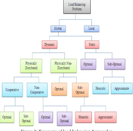
The taxonomy of load balancing approaches is presented for scheduling and load balancing algorithms in general purpose distributed computing systems. The organization of the different load balancing schemes is shown in Figure 2. 1) Local vs. Global: A distinction is drawn between local and global scheduling at the top level. The local scheduling discipline determines how the processes resident on a single CPU is residing and executed. A global scheduling policy uses information about the system to allocate processes to multiple processors to optimize a system-wide performance. Grid scheduling falls into the global scheduling branch.
Figure 2: Taxonomy of load balancing Approaches
2) Static versus Dynamic: The Static load balancing, also known as deterministic distribution, assigns a given job to a fixed resource. Every time the system is restarted, the same binding task resource is used without considering changes that may occur during the system lifetime. In this approach, every task comprising the application is assigned once to a resource. So, the placement of an application is static, and a firm estimate of the computation cost can be made in advance of the actual execution.
The Dynamic load balancing takes into account the fact that the system parameters may not be known beforehand. That’s why we don’t use a fixed or static scheme will eventually produce poor results.A dynamic stratgy gives good results rather then the static. A dynamic strategy is usually executed several times and may reassign a previously scheduled task to a new resource based on the current state of system environment [4].
The benefits of dynamic over static load balancing are that the system needs not be aware of the run-time behaviour of the application before execution. For dynamic strategies, the main problem is how to characterize the exact workload of a system, while it changes in a continuous way. Dynamic
strategies can be applied both for homogeneous or heterogeneous platforms with different degree of performances.
3) Optimal vs. Suboptimal: All information regarding the state of resources and the jobs is known, an optimal assignment could be made based on some criterion function, such as minimum makespan and maximum resource utilization. Due to the NP-Complete nature of scheduling algorithms and the difficulty in Grid scenarios to make reasonable assumptions which are usually required to prove the optimality of an algorithm, current research tries to find suboptimal solutions, which can be further divided into the following two general categories[5].
1. Approximate and 2. Heuristic.
4) Approximate vs. Heuristic: The approximate algorithms used in formal computational models, but instead of searching the entire solution space for an optimal solution, they are satisfied when a solution that is sufficiently good is found. In the case where a metric is available for evaluating a solution, this technique can be used to reduce the time taken to find an acceptable schedule.
5) Distributed vs. Centralized: The responsibility of dynamic load balancing is for making global decisions may lie with one centralized location, or be shared by multiple distributed locations.
The centralized strategy has the advantage for the implementation, but suffers from the lack of scalability, Fault tolerance and the possibility of becoming a performance bottleneck.
In distributed strategy, the state of resources is distributed among the nodes that are responsible for managing their own resources or allocating tasks residing in their queues to other nodes.
6) Cooperative vs. Non-cooperative: If a distributed load balancing mode is adopted then the next issue that should be considered is whether the nodes involved in job balancing are working independently or cooperatively. In the noncooperative case, an individual system load balancing acts as alone as autonomous entities and make the decisions regarding their own objectives independently of these decisions effects about the rest of the system.
C. Objective Functions of Load Balancing
The two major parties of Grid computing, namely resource consumers who submit various applications and resources providers who share their resources anddifferent motivations when they join the Grid. These incentives are presented by objective functions in scheduling. Grid users are basically concerned with the applications and their performance, for instance the total cost to run a particular application, while resource providers usually pay more attention to the resource’sperformance, for example the resource utilization in a particular period. Thus objective functions can be classified into two categories [6]:
1. Application-centric and
Figure 3: Objective Functions
1. Application-Centric: Load balancing algorithms usinging an application-centric objective function aim to optimize the individual application performance. Application centric is also known as the application level.
Most of current Grid applications concerns are about time, such as the make span and economic cost.
2. Resource-Centric: Load balancing algorithms also using resource-centric objective functions aim to optimize the resources performance. Resource centric is also known as the system level. Resource-centric objectives are usually related to resource utilization and economic profit, for example:
a) Throughput which is the ability of a resource to process a certain number of jobs in a given period.
b) Utilization, which is the amount of time, a resource is busy.
D. Types of Load Balancing Algorithms
Load Balancing Algorithms can be classified in two different ways:
1. Static Load Balancing Algorithm: The decisions related to load balance are made at compile time when resource requirements are estimated. The advantage of algorithm is the simplicity according to both implementation and overhead, since there is no need to constantly monitor the nodes for performance statistics.Static algorithms work properly only when nodes are having low variation in the load. Therefore these algorithms are not well suited for the grid environment, where load is varying at various times [7].
Figure 4: Static Load Balancing Algorithm
2. Dynamic Load Balancing Algorithm: Dynamic load balancing algorithms make changes to the distribution of work among nodes at run-time; they use current or load information when making distribution decisions [8].
Dynamic load balancing algorithms are advantageous over static algorithms. But to gain this advantage, we need to
consider the cost to collect and maintain the load information.
Figure 5: Dynamic Load Balancing Algorithm
A DLB algorithm considers following issues:
1. Load estimation policy, which determines how to
estimate the workload of a particular node of the system.
2. Process transfer policy, which determines whether to
execute a process locally or remotely.
3. State information exchange policy, which determines
how to exchange the system load information among the nodes.
4. Priority assignment policy, which determines the priority of execution of local and remote processes at a particular node.
5. Migration limiting policy, which determines the total
number of times a process, can migrate from one node to another.
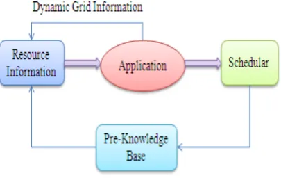
III PROPOSED SYSTEM ARCHITECTURE
We proposed a technique on the basis of load balancing in Grid environment, which dynamically balances the load. The rules generated by data mining techniques are used for migrating jobs for load balancing. Load balancing take place when some changes occurs in the load state. There are some particular tasks which change the load configuration in Grid environment which can be categorized as following:
Any new job arrived
Completion of execution of any job Any new resource arrived
Any existing resource withdrawal Machine failure at any node Node become overloaded
information from the database. The architecture of load balancing algorithm is presented in the figure 6.
Initial Status collect the information about all connected nodes like resource entry and job entry. Computation is done after the initial status.
Figure 6: System Architecture
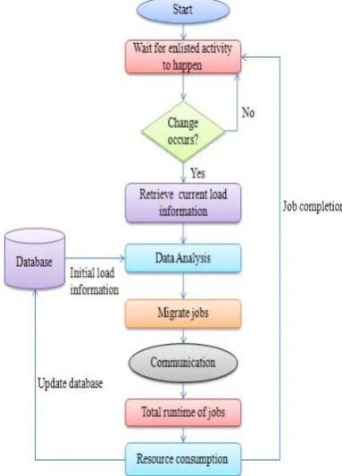
1) Following is the proposed algorithm for Adaptive Dynamic Load Balancing:
1. Initialize the status of all nodes. 2. Initial status=.Previous 3. While jobs=N N>0 do
4. if Current state is ready to change then
5. Current = Get change state (); //Computation stage 6. Threshold = generate threshold (upper bound, lower
bound); //Load Balancing
7. Migrate jobs (Previous,Current); //Partitioning
8. Communication SCM = Total message lengh+ Processing in each stage;
9. Total runtime of jobs is the sum of the four stages
(load balancing, computation, communication
and partitioning).
STotal = SDM + SCM + SCP + SLB
10. Resource consumption of a stages = ∑ Pi Ri
Pi = Processors
Ri = Run time for each processor
11. end if 12. end while 13. END
2) Variables Used: These variables are used in the algorithm A job defines number of tasks running on grid.
Current state indicates change in the state of load in grid. Current indicates current load status of all the nodes on
grid.
Previous indicates load status of all nodes on grid before the change in the state.
Threshold indicates maximum limit of handling load for each node on a grid.
3) Methods used: These methods are used in the algorithm. Get change state () to get the current status of load on
each node of grid.
Migratejobs (Previous, Current) to migratejobs as per the current and previous status of nodes.
Generate threshold (Upper bound, Lower bound) to find out new threshold values of each nodes of grid based on upper bound and lower bound limit.
Figure 7: Flowchart of Proposed Algorithm
data and send for receive messages. The last step is the load balancing, which is dynamic load balancing based on the time patterns. The total time spent on data movement, communication and load balancing can then be viewed as the overhead due to parallel processing. We define the threshold in the upper bound and lower bound. Upper bound means the load should not exceed more than two and lower bound is one. The load should not be less than one.
A. Comparative Analysis of Load Balancing
Algorithms
The comparative study of load balancing algorithms has been done on the basis of several qualitative parameters.
Table 1: Comparison Analysis of Load Balancing Algorithms
B. Implementation Details and Results
Load Balancing components have been developed which executes in simulated grid environment. This application has been developed using Java and SQLServer 2005 database server.
1) Grid Computing Environment Simulation Using GridSim
How a simulated Grid computing environment is created using GridSim. First, the Grid users and resources for the simulated Grid environment have to be created. This can be done easily using the wizard dialog as shown in Figure 8.
Figure 8: Wizard Dialog to Create Grid Users and Resources
The GridSim user only needs to specify the required number of users and resources to be created. Random properties can also be automatically generated for these users and resources. The GridSim user can then view and modify the properties of these Grid users and resources by activating their respective property dialog. To view the status of users click on view user button and respective dialog box displayed as shown in figure 9.
Figure 9: Wizard Dialog to view Grid Users
To view the status of resources click on view resource button and respective dialog box displayed as shown in figure 10.
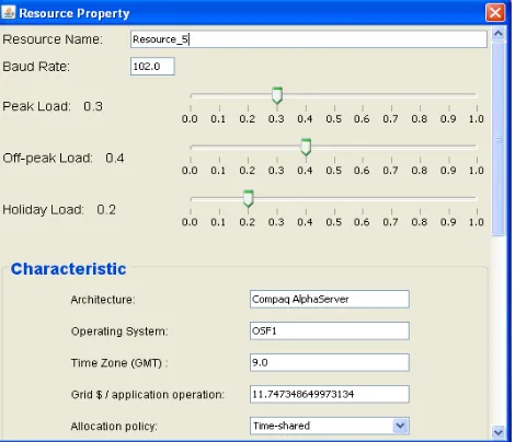
Figure 11 shows the property dialog of a sample Grid resource. GridSim creates Grid resources similar to those present in any other testbed. Resources of different capabilities and configurations can be simulated, by setting properties such as cost of using this resource, allocation policy of resource managers (time/space-shared) and number of machines in the resource with Processing Elements (PEs) in each machine and their Million Instructions per Second (MIPS) rating.
Figure 11: Resource Dialog to View Grid Resource Properties
Figure 12 shows the property dialog of a sample Grid user. Users can be created with different requirements (application and quality of service requirements). These requirements include the baud rate of the network (connection speed), maximum time to run the simulation, time delay between each simulation, and scheduling strategy such as cost and time optimization for running the application jobs. The application jobs are modeled as Gridlets.
Figure 12: User Dialog to View Grid User Properties
The parameters of Gridlets that can be defined include number of Gridlets, job length of Gridlets in Million
Instructions (MI), and length of input and output data in bytes. GridSim provides a useful feature that supports random distribution of these parameter values within the specified derivation range. Each Grid user has its own economic requirements (deadline and budget) that constrain the running of application jobs. GridSim supports the flexibility of defining deadline and budget based on factors or values.If it is factor-based (between 0.0 and 1.0), a budget factor close to 1.0 signifies the Grid user’s willingness to spend as much money as required. The Grid user can have the exact cost amount that it is willing to spend for the value-based option. GridSim will automatically generate Java code for running the Grid simulation .This file can then be compiled and run with the GridSim toolkit packages to simulate the required Grid computing environment.
2) Java Monitoring & Management Console
Java Monitoring & Management Console used to develop the memory usage, CPU load, classes and live threads in graphical foam.
Figure 13: Memory Usage
Figure 13 shows the Memory Usage Page. This page shows the used memory.
Figure 14: Number of Threads
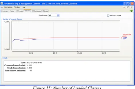
Figure 15: Number of Loaded Classes
Figure 15 shows the Number of Loaded Classes Page. This page shows the total classes and loaded classes.
Figure 16: Overview of all Classes
Figure 16 shows the Overview of Classes Page. This page shows the summary of heap memory usage, threads, classes and CPU load. Heap memory usage shows the used, commited and maxmium size of memory. Threads show the graph of live threads. Class’s shows the number of loaded classes.
IV CONCLUSION
This work focuses on design and implementations of Adaptive dynamic load balancing system for Grid computing environment. Proposed algorithm can use initial load information stored in the database at the initial level and current load information after load imbalance are first recorded.Grid application performance becomes a challenge in dynamic grid environment. Resources can be submitted to Grid and can be withdrawn from Grid at any time. These features of Grid make Load Balancing one of the critical features of Grid infrastructure. There are a number of factors, which can affect the grid application performance like load balancing, heterogeneity of resources and resource sharing in the Grid environment. The dynamic scheduling strategy of varying the number of processors during the lifetime of a parallel multistage computation can significantly affect the
total parallel runtime and total resource consumption. In adaptive computing the problem size varies during simulation. Varying the number of processors at runtime can be beneficial to low-power high-performance parallel system designs. Load Balancing is one of most important features of Grid Middleware for efficient execution of compute intensive applications. The efficiency of Load Balancing Module overall decides the efficiency of Grid Middleware.Proposed algorithm is executed in simulated Grid environment.
ACKNOWLEDGMENT
This research work was supported by Lovely Professional University Phagwara, India (LPU). The author is grateful to Asst. Prof. Harshpreet Singh for his discussions, advices and editing.
REFERENCES
[1] Pawandeep Kaur, Harshpreet Singh “Dynamic Load Balancing in Grid Environment using Adaptive computing”, International Conference on Recent Trends of Computer Technology in Academia (ICRTCTA-2012), April 2012.
[2] R. Buyya and J. Giddy and H. Stockinger, Economic Models for Resource Management and Scheduling in Grid Computing, in J. of Concurrency andComputation: Practice and Experience, Volume 14, Issue (13-15), Pages (1507-1542), Wiley Press, Dec. 2002.
[3] Ratnesh Kumar Nath, ”Efficient Load Balancing Algorithm in Grid Environment”, Thapar University, Patiala, May 2007.
[4] Belabbas Yagoubi and Yahya Slimani, ”Dynamic Load Balancing Strategy for Grid Computing”, World Academy of Science, Engineering and Technology 19, 2006.
[5] T.G. Casavant and J.L. Khul.‘Taxonomy of scheduling in general purpose distributed computing systems’.IEEE Transactions on Soft. Engineering, 14(2):pp.140-155, 1995.
[6] Y. Zhu, A Survey on Grid Scheduling Systems, Department of Computer Science, Hong Kong University of sci. and Tech., 2003.
[7] Javier Bustos Jimenez, ”Robin Hood: An Active Objects Load Balancing Mechanism for Intranet”, Departamento de Ciencias de la
Computacion, [email protected], Universidad de Chile.
[8] S. Iqbal, Load balancing strategies for parallel architectures, Ph.D. Thesis, Univeristy of Texas at Austin, May 2003.
![Figure 1: Job Migration [3] Load Balancing Policies](https://thumb-us.123doks.com/thumbv2/123dok_us/7820209.1295744/1.595.346.514.439.563/figure-job-migration-load-balancing-policies.webp)