Md O. F. Howlader* and Tariq P. Sattar
Abstract—In this paper, a one-dimensional numerical framework based on Finite-Difference Time-Domain (FDTD) method is developed to model response behaviour of Ground penetrating radar (GPR). The effects of electrical properties such as dielectric constant, conductivity of the media have been evaluated. A Gaussian shaped pulse is used as source which propagates through the 1D array grid, and the pulse interactions at different media interfaces have been investigated. The objective of this paper is to assess the modelling criteria and success rate of detecting buried object using the framework. A real life application of GPR to detect a buried steel bar in one meter thick concrete block has been carried out, and the results present successful detection of the steel bar along with measured depth of the concrete cover. The developed framework could be implemented to model multi-layer dielectric blocks with detection capability of various buried objects.
1. INTRODUCTION
Ground penetrating radar (GPR) is an electromagnetic (EM) technique based on the propagation, reflection and scattering of high frequency (10 MHz–2.5 GHz) waves in the subsurface. High resolution imaging of shallow subsurface can be achieved by using GPR. GPR has become a widely used non-destructive testing (NDT) equipment and found its application in areas such as concrete structures inspection, finding underground pipes and buried cables, determining the thickness and structure of ice glaciers, detecting buried containerized hazardous waste in petrochemical and nuclear industry [1]. GPR operation can be categorized in two main modes: (1) time-of-flight (ToF) based surveying where the transmitter and receiver antennas are located on the surface of the earth, and the imaging is done based on changes in electrical properties of the subsurface layers, and (2) borehole surveying, where one or both antennas are located in boreholes, and topographical subsurface properties are estimated [2]. A key performance factor of any GPR application is the penetration depth achieved or the lack of it which depends on the electrical characteristics of the object and of the material in which the object is buried. The penetration depth is rapidly attenuated in conductive lossy materials. In [3], experiments showed that high absorption of EM waves can be caused by presence of high moisture content in the propagating medium while the presence of salt water can cause total attenuation of the signals. Another big factor is the lack of clear reflectors due to the presence of an inhomogeneous medium which limits successful application of GPR to obtain valid information on the geometry of the structures and on the kind and size of existing faults in it [4].
Many methods have been developed until now to numerically simulate propagation of EM wave such as ray-based methods [5], frequency-domain methods [6], methods of moment (MoM) [7], finite element method (FEM) [8], and the finite-difference time-domain (FDTD) method [9]. FDTD has evolved as a powerful computational tool as the time-domain nature of FDTD-based programs enables the visualization of complex electromagnetic phenomena such as the propagation of electromagnetic
Received 3 September 2015, Accepted 29 October 2015, Scheduled 9 November 2015 * Corresponding author: Md Omar Faruq Howlader ([email protected]).
pulses in different media. FDTD algorithm is conceptually simple and accurate arbitrarily complex models. Moreover, FDTD results could assist in realistic antenna designs and their features such as dispersion in electrical properties. Also FDTD provides good scalability compared with other popular electromagnetic modelling methods such the FEM and integral MoM techniques [10].
In this paper, a numerical framework for GPR modelling based on FDTD is developed. FDTD method has been used to model GPR scenarios which involve wave propagation in complex media such as nonhomogeneous, lossy, dispersive and non-linear media and objects of arbitrary shape. Effect of parameters such as electric permittivity, magnetic permeability and conductivity of medium on EM wave propagation have been investigated, and a real life GPR application of detecting and measuring the depth of a steel reinforced bar (rebar) buried under a concrete cover has been presented. This paper presents a version of FDTD code which is based on developed framework and has been implemented in MATLAB to model and simulate a GPR’s performance. A computationally intensive full 3D model provides a complete view of waves scattering and interactions. However, due to the large amount of book-keeping required in any full 3D-FDTD code, the dimensionality has been reduced to 1D for better understanding of the framework.
A considerable amount of research was devoted to FDTD for material dispersion behaviour, complex geometrical shapes, antenna design and so on. However, most of those works are limited to specific medium and its behaviour, very specific problem dimensions, etc. Also many of those only emphasize the obtained results rather than through discussion of the algorithm. This paper breaks down the building block of the FDTD algorithm and proposes a framework for collective application of the system. Here only one framework can be implemented to model a variety of media by alternating the electric and magnetic property variables in the framework. This can help researchers to simplify their research questions and gather data from wide range of materials and media. Moreover, simulation results acquired from this framework can provide an overview of the total problem scenario of real life GPR application. These results are vital to establish the responses expected from physical GPR application. Furthermore, the subsequent stages of designing antenna and transceiver system for the GPR could be fine-tuned for better accuracy by following those results.
The paper consists of the following sections. Section 2 gives an overview of the GPR operation. Section 3 describes the formulation of FDTD equations and numerical framework. MATLAB implementation and numerical testing of the algorithm is presented in Section 4, and finally, the paper concludes with a brief summary and recommendation in Section 5.
2. BASIC PRINCIPLES OF GPR
GPR can offer non-destructive subsurface mapping, and the most important advantage of GPR is its resolution which is usually higher than the other NDT techniques. By using pulse generators of short pulses in nanosecond region, GPR can achieve higher resolution to detect buried objects of centimetre or moreover millimetre scale [11]. A typical GPR is composed of transmitting and receiving antennas, a timing and control unit, a data storage unit, a graphic display unit, and a power supply unit as in Figure 1.
The function of the transmitting antenna is to emit an EM pulse into the ground which is partly reflected when it encounters inhomogeneous media with different dielectric properties and partly transmitted into deeper layers. A receiving antenna located in either a separate antenna box or in the same antenna box as the transmitter as Figure 2 records the reflected signal.
A timing circuit processes the time difference, and the reflection data may be composed in 3 different forms, namely A-scans, B-scans, and C-scans and is shown in the display. The A-scan is a stationary measurement from a specific position on the surface, presented in the form of a time-series signal and is used in this paper. A set of A-scans builds a B-scan image, and a group of B-scan images forms a 3D C-scan data cube [12]. Typical velocities of EM pulses vary in different materials, which is reported in [13]. The reason for most important velocity changes depends on the presence of inhomogeneities in the medium and on the moisture content [14]. Therefore, once the wave velocity is calibrated for a specific medium, a depth scale can be calculated by the GPR.
Figure 1. Block diagram of a GPR system. Figure 2. Transmitting and receiving antennas of a commercial GSSI GPR.
environmental variables that must be modelled in a GPR simulation for a realistic modelling include the characteristics: permittivity, ε, conductivity, σ, and permeability, μ, of the air above the surface, the subsurface, and the target.
3. FDTD BASED FRAMEWORK FOR GPR MODELLING
Maxwell’s electromagnetic equations that mathematically express the relations between the fundamental electromagnetic field quantities and their dependence on their sources can be used to describe all electromagnetic phenomena. The fundamental equations are:
∇ ×E = −μr
C0 ∂H
∂t (1)
∇ ×H = εr
C0 ∂E
∂t (2)
wheretis time (seconds), andεr,μr are the relative permittivity, relative permeability of the medium, respectively, and are usually referred to as the constitutive parameters. These parameters are functions of position, direction, the strength of the applied field and time and they couple the flux quantities with the electric and magnetic field intensities. From Equations (1) and (2), three-dimensional partial differential equations of Maxwell’s equations can be written as:
∂Ez
∂y −
∂Ey
∂z = −
1
C0
μxx∂Hx ∂t +μxy
∂Hy ∂t +μxz
∂Hz ∂t (3) ∂Ex ∂z − ∂Ez
∂x = −
1
C0
μyx∂Hx ∂t +μyy
∂Hy ∂t +μyz
∂Hz ∂t (4) ∂Ey ∂x − ∂Ex
∂y = −
1
C0
μzx∂Hx ∂t +μzy
∂Hy ∂t +μzz
∂Hz ∂t (5) ∂Hz ∂y − ∂Hy ∂z = 1 C0
εxx∂Ex ∂t +εxy
∂Ey ∂t +εxz
∂Ez ∂t (6) ∂Hx ∂z − ∂Hz ∂x = 1 C0
εyx∂Ex ∂t +εyy
∂Ey ∂t +εyz
∂Ez ∂t (7) ∂Hy ∂x − ∂Hx ∂y = 1 C0
εzx∂Ex ∂t +εzy
∂Ey ∂t +εzz
∂Ez ∂t
(8)
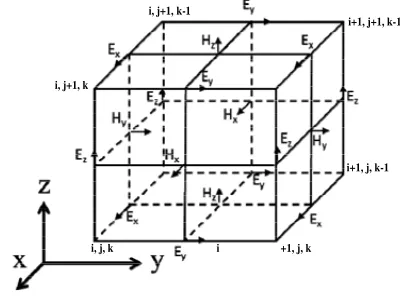
implemented to numerically solve Maxwell’s equations by discretizing them in both the space and time continua. As a result, the resolution of spatial and temporal discretization steps play a very significant role since higher resolution can provide FDTD model closer to a real representation of the problem. However, due to limited amount of storage and finite computing speed, the values of the discretization steps always have to be finite. Hence, the FDTD model represents limited size of a discretized version of the real problem. The building block of this discretized FDTD grid was first proposed by Kane Yee in 1966 and is called the Yee cell. The 3D Yee cell is illustrated in Figure 3.
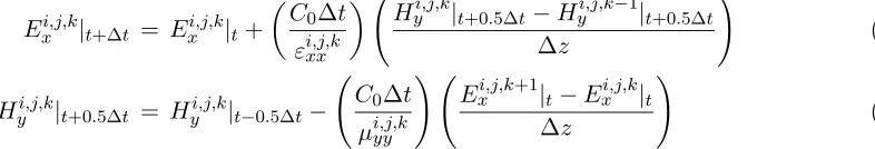
The solutions of general class of problems can be handled robustly using Yee algorithm which mimics the cyclic principle of a time varying electric (E) field producing a time vary magnetic (H) field and a time varying magnetic field producing a time vary electric field in turn. According to the algorithm, theE andH fields are half time step away from each other as shown in Figure 4, and taking that as a guide, the discretization equations of Maxwell’s equations for diagonal anisotropic material could be formulated as below,
Ezi,j+1,k|t−Ezi,j,k|t
Δy −
Eyi,j,k+1|t−Ei,j,ky |t
Δz =−
μi,j,kxx C0
Hxi,j,k|t+0.5Δt−Hxi,j,k|t−0.5Δt
Δt (9)
Exi,j,k+1|t−Exi,j,k|t
Δz −
Ezi+1,j,k|t−Ezi,j,k|t
Δx =−
μi,j,kyy C0
Hyi,j,k|t+0.5Δt−Hyi,j,k|t−0.5Δt
Δt (10)
Eyi+1,j,k|t−Eyi,j,k|t
Δx −
Exi,j+1,k|t−Ei,j,kx |t
Δy =−
μi,j,kzz C0
Hzi,j,k|t+0.5Δt−Hzi,j,k|t−0.5Δt
Δt (11)
Hzi,j,k|t+0.5Δt−Hzi,j−1,k|t+0.5Δt
Δy −
Hyi,j,k|t+0.5Δt−Hyi,j,k−1|t+0.5Δt
Δz =
εi,j,kxx C0
Exi,j,k|t+Δt−Exi,j,k|t
Δt (12)
Hxi,j,k|t+0.5Δt−Hxi,j,k−1|t+0.5Δt
Δz −
Hzi,j,k|t+0.5Δt−Hzi−1,j,k|t+0.5Δt
Δx =
εi,j,kyy C0
Eyi,j,k|t+Δt−Eyi,j,k|t
Δt (13)
Hyi,j,k|t+0.5Δt−Hyi−1,j,k|t+0.5Δt
Δx −
Hxi,j,k|t+0.5Δt−Hxi,j−1,k|t+0.5Δt
Δy =
εi,j,kzz C0
Ezi,j,k|t+Δt−Ezi,j,k|t
Δt (14)
In this paper, problems composed of dielectric layers will be derived in just one dimension. In this case, the materials and the fields are uniform in any two directions, hence, derivatives in these uniform directions will be zero. If the uniform directions are to be theX andY axes, then the electromagnetic wave propagation behaviour will be as in Figure 5.
Therefore, the three-dimensional equations from Equations (9) to (14) could be scaled down to one dimensional equation by substituting Δx = Δy = 0. Here, the longitudinal field components,Ez and
i, j+1, k
i, j+1, k-1
i, j, k i +1, j, k
i+1, j, k-1 i+1, j+1, k-1
Figure 5. 1D array of Yee cell.
Hz, are always found to be zero, and the Maxwell’s equations decouples into two sets of equations:
Exi,j,k+1|t−Ei,j,kx |t
Δz = −
μi,j,kyy C0
Hyi,j,k|t+0.5Δt−Hyi,j,k|t−0.5Δt
Δt (15)
−Hyi,j,k|t+0.5Δt−Hyi,j,k−1|t+0.5Δt
Δz =
εi,j,kxx C0
Exi,j,k|t+Δt−Exi,j,k|t
Δt (16)
Eyi,j,k+1|t−Ei,j,ky |t
Δz =
μi,j,kxx C0
Hxi,j,k|t+0.5Δt−Hxi,j,k|t−0.5Δt
Δt (17)
Hxi,j,k|t+0.5Δt−Hxi,j,k−1|t+0.5Δt
Δz =
εi,j,kyy C0
Eyi,j,k|t+Δt−Eyi,j,k|t
Δt (18)
Equations (15) and (16) together is called Ex/Hy mode, and Equations (17) and (18) together is called Ey/Hxmode. These two modes will propagate independently in physical medium; however, numerically
they are the same and will exhibit identical electromagnetic behaviour. Therefore, it is only necessary to solve only one mode. In this paper, Ex/Hy mode is solved for numerical modelling. Therefore, two
updated equations forEx/Hy mode and basic framework for 1D FDTD for GPR can be written as:
Exi,j,k|t+Δt = Exi,j,k|t+
C0Δt εi,j,kxx
Hyi,j,k|t+0.5Δt−Hyi,j,k−1|t+0.5Δt
Δz
(19)
Hyi,j,k|t+0.5Δt = Hyi,j,k|t−0.5Δt−
C0Δt μi,j,kyy
Exi,j,k+1|t−Exi,j,k|t
Δz
(20)
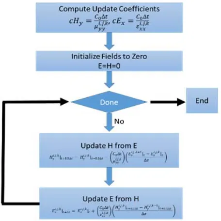
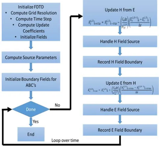
With a high level programming language such as MATLAB where array indexes can be declared, a script can be developed by the following bare bone structure of 1D FDTD algorithm as Figure 6.
3.1. Source
Energy in the form of Gaussian or sinusoidal wave is injected in the grid cell to initiate the FDTD algorithm. Source is usually assigned as values to Ex at the boundary z = 0, k = 1. In order to
simulate a broad range of frequencies, pulses in Gaussian form are widely used. A Gaussian pulse centred at t0 is defined by,
g(t) =e
−
t−t0 τ
2
(21)
where, τ is the pulse width (s). Multiplying a sinusoidal wave equation to Equation (21) produces a sine modulated Gaussian source. It is good practice to have t0 = 5×τ so that the Gaussian pulse is
centred at half of the total 5 cycles of the modulation signal. Figure 7 shows a sine modulated Gaussian pulse.
Ex(t) = sin (2πf0t)e
−
t−t0 τ
2
Figure 6. Basic numerical framework for 1D FDTD algorithm.
Figure 7. Modulation of a Gaussian pulse using 0.6 PHz sinusoidal wave.
3.2. Boundary Conditions
Modelling open boundary problems like GPR faces an issue of truncation of the computational domain at a finite distance from the sources and targets as the electromagnetic fields cannot be calculated directly by the numerical method at the boundary. As FDTD 1D array has a finite number of cell, the outgoing Gaussian pulse will come to the edge of the model after certain period. If any special boundary condition is not defined then unpredictable reflections would be generated at the boundary that would go back inward and as a result there will be no way of determining real wave from the reflected one. The reflections are due to the intrinsic impedances of the media boundary and a solution is to make an adaptation such as absorbing boundary conditions (ABC) between them that the reflection coefficient would be zero and no reflection would occur [15]. These ABC’s will absorb any wave hitting the boundaries, hence will emulate an infinite space. In FDTD as the fields at the edge are propagating outward and it takes two time steps for the field to cross one cell therefore, the field value at the end can be estimated by the following equation.
Exk=Ekx−2(1) (23)
However, numerical imperfections might exist in ABC and reflections might still travel backward from the termination of medium at the truncation boundaries of the model. But they are easily distinguishable from the actual reflections from targets inside the model as those reflection will have significantly small amplitude compared to target reflections.
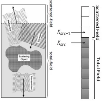
3.3. Total Field/Scattered Field
The source equations described earlier are for two-directional sources whereas, total-field/scattered-field (TF/SF) is a technique to inject a one directional source. Ay system grid could be divided into two regions as Figure 8 where the total field contains the source field and the field scattered from any target. But the scattered field can pass through source injecting point transparently into the scattered field region. This ensures waves at the boundaries are only travelling outwards and entire energy injected by the source is incident on the medium that is being simulated.
Figure 8. Wave propagation on a TF/SF grid. Figure 9. Correlation between electric and magnetic field.
scattered or both total) then Equations (19)–(20) can be used to update the corresponding field in time. However, as the field on the top of the source injection point is intended to be the scattered field and the bottom to be the total field,E and H field updated equations at ksrc point becomes,
Exi,j,ksrc|t+Δt = Exi,j,ksrc|t+
C0Δt εi,j,ksrcxx
Hyi,j,ksrc|t+0.5Δt−Hyi,j,ksrc−1|t+0.5Δt
Δz
(24)
Hyi,j,ksrc−1|t+0.5Δt = Hyi,j,ksrc−1|t−0.5Δt−
C0Δt μi,j,ksrcyy
Exi,j,ksrc|t−Exi,j,ksrc−1|t
Δz
(25)
Looking at the Ex field updated Equation (24) which is located on the total field side, the term Hyi,j,ksrc−1|t+0.5Δtis located on the scattered field side. For consistency, all terms of an updated equation
should be located on the same side of fields. Therefore, a magnetic field source is added to the term to turn all terms to total-field quantities, and the update equation becomes,
Exi,j,ksrc|t+Δt=Exi,j,ksrc|t+
C0Δt εi,j,ksrcxx
⎡
⎣H
i,j,ksrc
y |t+0.5Δt−
Hyi,j,ksrc−1|t+0.5Δt+Hyi,j,ksrc−1|srct+0.5Δt
Δz
⎤
⎦ (26)
Likewise, Equation (25), which is located on the scattered field side, has a termExi,j,ksrc|tfrom the total field side. To convert all the terms to scattered field quantities, an electric field is subtracted from the term as below,
Hyi,j,ksrc−1|t+0.5Δt=Hyi,j,ksrc−1|t−0.5Δt−
C0Δt μi,j,ksrcyy
⎡ ⎣
Exi,j,ksrc|t−Ei,j,ksrcx |srct
−Exi,j,ksrc−1|t
Δz
⎤
⎦ (27)
The above formulations show that original update Equations (19), (20) stay the same with added correction term Hyi,j,ksrc−1|srct+0.5Δt and Exi,j,ksrc|srct in Equations (26), (27) which needs to be defined. The way to achieve those correction terms is to define the electric field, Ex which is a Gaussian pulse
as Equation (24) in this case and then derive the magnetic field source with a phase shift, Hy using
Maxwell’s equations. So from Maxwell’s equations,
Exi,j,ksrc|srct = g(t) (28)
Hyi,j,ksrc−1|srct+0.5Δt =
εi,j,ksrcr
μi,j,ksrcr g
t+nsrcΔz 2×C0 −
Δt
2
where,
εi,j,ksrcr
μi,j,ksrcr is the amplitude of the magnetic field based on Maxwell’s equations,nsrcthe refractive index of the medium at the point of source injection and Δ2t the phase shift with the electric field. The corresponding electric and magnetic field is shown in Figure 9 which shows a phase shift of 3.7 ps for a 1 GHz Gaussian pulse.
3.4. Propagation in a Lossy Medium
The E and H field update equations derived in the previous sections are for free space medium by neglecting any loss term. However, to model a realistic GPR, the loss term of the medium must be incorporated in the update equations. In many media, loss term is specified by the conductivity, σ
term. This loss term results in the attenuation of the propagating energy of the electromagnetic wave through the medium. According to Maxwell’s curl equations to incorporate conductivity,
∇ ×H =η0σE+ εr C0
∂E
∂t (30)
Here,η0 is free space impedance. By discretizing and taking the spatial derivatives of Equation (30) in
the same way as described previously, the new update equation can be formulated as:
Exi,j,k|t+Δt=
2ε0εi,j,kxx −Δtσxxi,j,k
2ε0εi,j,kxx + Δtσxxi,j,k
Exi,j,k|t+
2ε0c0Δt
2ε0εi,j,kxx + Δtσxxi,j,k
Hyi,j,k|t+0.5Δt−Hyi,j,k−1|t+0.5Δt
Δz
(31)
If conductivity, σ is set to zero in Equation (31), then the equation reverts to initial Equation (19). Moreover, incorporating conductivity term into the system does not affect the magnetic field update equation. The pseudo programming code for the finalE andH filed update equations could be written as:
Ex[k] = (cEx1)Ex[k] + (cEx2) (Hy[k−1]−Hy[k])/dz (32) Hy[k] = Hy[k]−(cHy) (Ex[k+ 1]−Ex[k])/dz (33) Here, cEx1, cEx2, cHy are the constant coefficients, and they could be calculated before the final loop
of the program starts. The final numerical framework of FDTD could be achieved by combining all
space discretization size, Δz= 0.003 m and time step, Δt= 5.5 ps. The source of Gaussian pulse with centre frequency of 1.5 GHz is used to represent the current excitation of a line source representing the GPR transmitter in these models.
4.1. Validation of ABC
A lossless dielectric medium with εr = 1 is simulated first where the Gaussian pulse is injected at cell number 385 along the dotted vertical line travels outward. Propagation of both electric and magnetic fields are shown in Figure 11. Total number of iteration is 19068 which is 3 times higherthan required for total convergence of the simulation. At 5650th iteration, the signal hits the boundary line. But as the boundary is perfectly absorbing therefore, the wave does not reflect after hitting the boundary. As the wave completely passes the problem window at later iterations, there is no reflected wave present which validates successful implementation of ABC.
Figure 11. EM wave propagation through ABC.
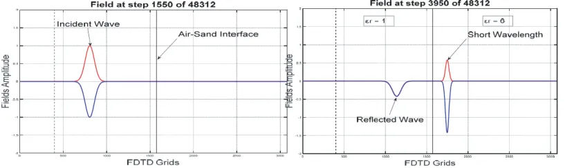
4.2. Propagation through Dielectric Medium
Figure 12 shows the simulation of the propagation, first in the air and then in the dry sand with dielectric constant ofεr= 6 after crossing the air — sand interface at cell number 1570. When the wave encounters the dielectric medium, a part of it is transmitted, and the other part is reflected. Moreover, the wavelength in sand is shorter than the wavelength in air, also the electric field amplitude reduces and changes polarity as the wave enters sand medium. Furthermore, by calculating the time difference between the incident wave and reflected wave at the source injection point, the distance of the air-sand interface from source point could be determined, which is a fundamental feature of GPR.
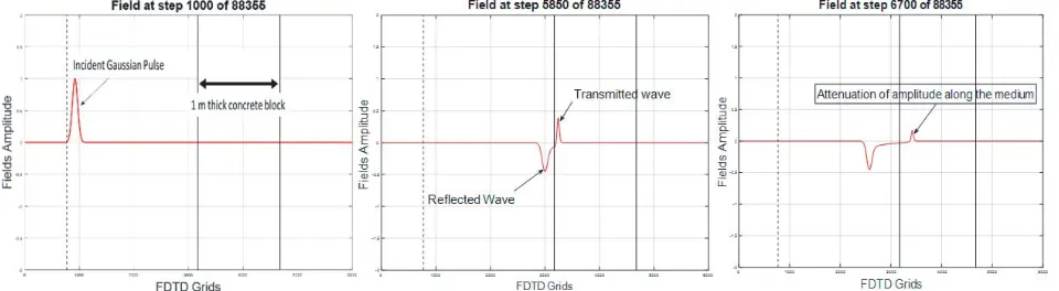
4.3. Applying FDTD Method to Simulate Reinforced Concrete Wall
Here FDTD is implemented to simulate a real application of GPR to detect reinforced buried rebar on a concrete wall. The medium used in the simulations corresponds to a homogenous medium (dry concrete with dielectric properties εr = 5.5, σ = 0.043 S/m). First a 1 m thick concrete wall is modelled in the system to observe wave propagation behaviour on a lossy concrete medium. The space discretization, Δzis set to 0.0014 m and time step, Δtto 2.3 ps. Length of the total model is 8.6 m simulated in centre frequency of 1.5 GHz. Figure 13 shows the model setup, and it is noticeable that a part of the wave reflected from the air-concrete interface and also the magnitude of the transmitted wave attenuates this time in the medium. This feature simulates the characteristic of any lossy medium.
Next, a steel rebar has been planted in the concrete block. Steel is a highly conductive metal, and as a result, the electric field value inside steel or any conductive metal is zero. Therefore, it should have infinite dielectric constant i.e., acts as perfect electric conductor. But ideally, no metals are perfect conductor as they have a portion of impurity in them. The permittivity for real metal is purely negative
Figure 13. Propagation of electric field in a lossy concrete medium.
right side of the rebar which indicates that 100% of the wave has been reflected although with reduced amplitude. By measuring the time of flight (ToF) of the two reflected pulses, the thickness of the concrete cover can be determined.
In FDTD algorithm, electromagnetic wave propagates one cell in two time steps and recorded two-way travel time of the reflected pulses in MATLAB are, 1st reflected pulse = 2.26×10⁻⁸s, 2nd reflected pulse = 2.46×10⁻⁸s. Therefore, time difference between the two reflected pulses to reach
back the source injection point is 0.1×10⁻⁸s, and from that the measured concrete cover is 0.3 m which
completely matches with the initial simulation model setup.
5. CONCLUSION
Either analytical or numerical modelling of electromagnetic wave propagation is essential for advanced understanding of GPR responses. This may help to develop new techniques for data processing and interpretation. Therefore, FDTD based modelling could offer both researchers and practitioners a low cost practical way of creating mathematical model. The numerical framework developed in this paper is directly derived in the time domain by using a discretized version of Maxwell’s curl equations that are applied in each FDTD cell. The solutions are obtained in iterative fashion where the electromagnetic fields advance in the FDTD grid, and each iteration corresponds to an elapsed simulated time of one Δt. The EM wave propagation in different media showed that the amplitude of the wave deteriorated significantly in medium with lossy conductivity. It showed the effect of electrical properties of medium on wave propagation. A real life application of GPR was considered to detect a steel rebar buried under a concrete cover. The time domain data were successful to detect the rebar based on reflected wave and by measuring time-of-flight of the reflected wave, and the depth of the rebar was calculated to be 30 cm which matched with initial model setup. Even though the paper discusses a 1D FDTD algorithm for GPR simulation, the versatility of the framework means that this framework could be used to model a wide variety of media, materials and problem scenarios. Further works involve incorporating more than two media into the system and create a 2D grid to generate a radargram of the subsurface mapping.
REFERENCES
1. Ji, G., X. Gao, H. Zhang, and T. Gulliver, “Subsurface object detection using UWB ground penetrating radar,” IEEE Pacific Rim Conference on Communications, Computers and Signal Processing, Victoria, Canada, 2009.
2. Irving, J. and R. Knight, “Numerical modeling of ground-penetrating radar in 2-D using MATLAB,” Journal of Computers & Geosicences, Vol. 33, 1247–1258, 2006.
3. Colla, C., D. McCann, and M. Forde, “Radar testing of a masonry composite structure with sand and water backfill,” Journal of Bridge Engineering, Vol. 6, No. 4, 262–270, 2001.
4. Diamanti, N., A. Giannopoulos, and M. C. Forde, “Numerical modelling and experimental verification of GPR to investigate ring separation in brick masonry arch bridges,” NDT & E International, Vol. 41, No. 5, 354–363, 2008.
5. Bergmann, T. and K. Holliger, “Numerical modeling of borehole georadar data,” Journal of Geophysics, Vol. 67, No. 4, 1249–1257, 2002.
7. Balanis, C., Antenna Theory: Analysis and Design, John Wiley and Sons, Inc., New York, 2005. 8. Jin, J., The Finite Element Method in Electromagnetics, 2nd edition, Wiley-IEEE Press, 2002. 9. Seyfi, L. and E. Yaldz, “A simulator based on energy-efficient GPR algorithm modified for the
scanning of all types of regions,”Turkish Journal of Electrical Engineering and Computer Sciences, Vol. 20, No. 3, 381–389, 2010.
10. Giannopoulos, A., “Modelling ground penetrating radar by GprMax,”Journal of Construction and Building Materials, Vol. 19, 755–762, 2005.
11. Perez-Gracia, V., D. Capua, R. Gonzalez-Drig, and L. Pujades, “Laboratory characterization of a GPR antenna for high-resolution testing: Radiation pattern and vertical resolution,”NDT &E International, Vol. 42, 336–344, 2009.
12. Malhotra, V. and N. Carino,Nondestructive Testing of Concrete, CRC Press, Florida, 2004. 13. Baker, G., S. Jordon, and J. T. Pardy, “An Introduction to ground penetrating radar (GPR),”The
Geological Society of America (Special Paper), Vol. 432, No. 2, 2007.
14. Binda, L., A. Saisi, C. Tiraboschi, S. Valle, C. Colla, and M. Forde, “Application of sonic and radar tests on the piers and walls of the Cathedral of Noto,”Journal of Construction and Building Materials, Vol. 17, No. 8, 613–627, 2003.