Scholarship@Western
Scholarship@Western
Electronic Thesis and Dissertation Repository
12-13-2017 2:45 PM
Study of Motion of Agglomerates Through a Fluidized Bed
Study of Motion of Agglomerates Through a Fluidized Bed
Muhammad Owais Iqbal Bhatti
The University of Western Ontario
Supervisor Briens, Cedric
The University of Western Ontario Co-Supervisor Berruti, Franco
The University of Western Ontario
Graduate Program in Chemical and Biochemical Engineering
A thesis submitted in partial fulfillment of the requirements for the degree in Master of Engineering Science
© Muhammad Owais Iqbal Bhatti 2017
Follow this and additional works at: https://ir.lib.uwo.ca/etd
Part of the Other Chemical Engineering Commons
Recommended Citation Recommended Citation
Bhatti, Muhammad Owais Iqbal, "Study of Motion of Agglomerates Through a Fluidized Bed" (2017). Electronic Thesis and Dissertation Repository. 5066.
https://ir.lib.uwo.ca/etd/5066
This Dissertation/Thesis is brought to you for free and open access by Scholarship@Western. It has been accepted for inclusion in Electronic Thesis and Dissertation Repository by an authorized administrator of
i
Formation of agglomerates in Fluid CokersTM can cause operating problems, such as excessive
shed fouling, which can lead to premature unit shut down. Better understanding of how
agglomerates move through a fluidized bed can help improve the design and operation of Fluid
CokersTM and minimize the risk of agglomerates reaching regions where they cause problems.
To identify key factors in agglomerates motion in a fluidized bed, a new two-dimensional (2D)
Radioactive Particle Tracking (RPT) method was developed which tracks model agglomerates
motion. In conjunction, a tribo-electric method was used to determine bubble flow distribution
in the fluidized bed.
This thesis outlines the effects of bed hydrodynamics and agglomerate properties on
agglomerate motion. It was found that agglomerates produced by liquid injection in the
fluidized bed were of similar density. Agglomerates larger than 9500 µm segregated near the
bottom of the fluidized bed and all agglomerates spent more time in regions of low bubble
flow.
Keywords
Fluid Coking, Fluidized Bed, Radioactive Particle Tracking, Motion of Agglomerates,
ii
Co-Authorship Statement
Chapter 3
Article Title: Preliminary Study on Behavior of Agglomerates formed by Liquid Injection
Authors: Muhammad Owais Iqbal Bhatti, Cedric Briens, Franco Berruti, Jennifer McMillan.
Article Status: Unpublished
Contributions:
Muhammad Owais Iqbal Bhatti wrote the manuscript who also conducted all the
experimental work and data analysis. Cedric Briens and Franco Berruti jointly supervised
the work. Cedric Briens, Franco Berruti and Jennifer McMillan reviewed several drafts of
the chapter.
Chapter 4
Article Title: Development of a New Two-Dimensional Radioactive Particle Tracking (RPT) System to Study the Motion of Agglomerates
Authors: Muhammad Owais Iqbal Bhatti, Francisco J. Sanchez, Cedric Briens, Franco Berruti, Jennifer McMillan.
Article Status: Unpublished
Contributions:
Muhammad Owais Iqbal Bhatti wrote the manuscript who also conducted all the
experimental work and data analysis. Franciso J. Sanchez provided assistance and guidance
in setting up the RPT system. Cedric Briens, Franco Berruti and Jennifer McMillan reviewed
iii
Chapter 5
Article Title: Study of the Impact of Radial Fluidization Gas Profile on Agglomerates Motion
Authors: Muhammad Owais Iqbal Bhatti, Cedric Briens, Franco Berruti, Jennifer McMillan.
Article Status: Unpublished
Contributions:
Muhammad Owais Iqbal Bhatti wrote the manuscript who also conducted all the
experimental work and data analysis. Cedric Briens and Franco Berruti jointly supervised
the work. Cedric Briens, Franco Berruti and Jennifer McMillan reviewed several drafts of
the chapter.
iv
Acknowledgments
Conducting research at ICFAR was one of the toughest challenges of my life so far and this
journey would not have been possible without the incredible people who guided and supported
me during this time.
I could not be more grateful to my supervisors, Dr. Cedric Briens and Dr. Franco Berruti, for
giving me the prestigious opportunity to work at ICFAR. Both of whom not only shared their
expertise and in-depth knowledge with me but also provided the guidance, constructive
criticism and constant motivation that was needed to complete this challenging task.
I would like to thank Syncrude Canada Limited and Natural Sciences and Engineering
Research Council (NSERC) of Canada for the financial support. Also, I am grateful to Province
of Ontario and The University of Western Ontario for providing me with the funds through
Queen Elizabeth II – Graduate Scholarship in Science and Technology (QEII-GSST).
I am especially indebted to Dr. Francisco J. Sanchez and Majid Jahanmiri, who both put in
countless efforts in helping me setup the equipment required for the research. I would also like
to thank Thomas Johnston and Cody Ruthman (from University Machine Services) for helping
me with the modifications in the unit and navigating through the technical problems. I would
also like to express my gratitude and appreciation to all my friends, colleagues and personnel
at ICFAR, especially Saber, Dhiraj, Cher, Afsana, Chiara, Marina, Luanna, Muhammad, Tracy
and Stefano for all the great memories I would cherish my whole life.
In the end, this wonderful voyage would be meaningless if it wasn’t for my parents and family.
I am very fortunate to get all the love, support and courage from my Papa Mr. Muhammad
Iqbal Bhatti, my Ammi Mrs. Shahida Iqbal, my beloved sister Sidra Iqbal and my brothers
Junaid Iqbal, Fahad Iqbal, Saad Iqbal and Abdur-Rehman Iqbal.
This page would be incomplete without mentioning my best friends Nazim Hussain, Faizan
Siddiqui, Danish Ali, Sana Zahid, Baber Rahim, Kiran Baber, Tauseef, Manzar, Sufyan Khan
v
Table of Contents
Abstract ... i
Co-Authorship Statement... ii
Acknowledgments... iv
Table of Contents ... v
List of Tables ... ix
List of Figures ... x
List of Appendices ... xx
Nomenclature ... xxi
Chapter 1 ... 1
1 Introduction ... 1
1.1 Bitumen ... 1
1.2 Coking ... 2
1.3 Fluid Coking ... 2
1.3.1 Fouling ... 4
1.3.2 Sheds ... 4
1.4 Agglomeration ... 5
1.4.1 Formation of Agglomerates ... 6
1.5 Models for the Study of Agglomerate Formation ... 7
1.6 Tribo-Electric Method for Bubble Flow Distribution ... 8
1.6.1 Theory and Background ... 8
1.7 Radioactive Particle Tracking ... 9
1.7.1 Theory and Background ... 9
1.7.2 Factors Affecting Strength of Radioactive Source ... 10
vi
1.7.4 Rendition Techniques ... 13
1.8 Research Objectives and Outline ... 14
Chapter 2 ... 16
2 Experimental Setup and Methodology ... 16
2.1 Equipment ... 16
2.2 Fluidized Bed ... 17
2.3 Liquid Injection System ... 18
2.4 Agglomerates Recovery ... 19
2.5 Agglomerates Analysis ... 20
2.6 Tribo-Electric Method ... 21
2.6.1 Analysis of Triboelectric Signals ... 23
2.7 Radioactive Particle Tracking (RPT) System ... 23
2.7.1 Radioactive Particle/Source ... 24
2.7.2 Scintillation Detectors ... 24
2.7.3 Experimental Setup ... 27
Chapter 3 ... 30
3 Preliminary Study on Behavior of Agglomerates formed by Liquid Injection ... 30
3.1 Bubble Flow Distribution in the Fluidized Bed ... 30
3.2 Experimental Setup and Procedure ... 30
3.2.1 Data Acquisition for Triboelectric Method ... 33
3.3 Results and Discussion ... 33
3.3.1 Results for Vertical Distribution of Agglomerates ... 33
3.3.2 Results for Lateral Distribution of Agglomerates ... 43
3.3.3 Density of Agglomerates ... 49
3.3.4 Gas Bubble Flow Distribution using Tribo-Electric Method ... 50
vii
Chapter 4 ... 58
4 Development of a New Two-Dimensional Radioactive Particle Tracking System to Study the Motion of Agglomerates ... 58
4.1 Experimental Setup and Procedure ... 58
4.1.1 Development of a New Method for 2D RPT System ... 59
4.1.2 Preparation of Model Agglomerates ... 68
4.1.3 Experimental Procedure ... 70
4.2 Results and Discussion ... 70
4.2.1 Results for Model Agglomerate-2 (12500 µm) ... 70
4.2.2 Results for Model Agglomerate-1 (5500 µm) ... 78
4.2.3 Comparison of Results Obtained with Agglomerates formed by Liquid Injection Experiments with RPT Results ... 86
4.3 Conclusion ... 92
Chapter 5 ... 94
5 Study of the Impact of Radial Fluidization Gas Profile on Agglomerates Motion ... 94
5.1 Experimental Setup and Procedure ... 94
5.2 Results and Discussion ... 95
5.2.1 Gas Bubble Flow Distribution using Tribo-Electric Method ... 95
5.2.2 Results for Liquid Injection Experiments ... 99
5.2.3 Results for Radioactive Particle Tracking ... 105
5.2.4 Comparison of Results obtained with Agglomerates formed by Liquid Injection Experiments, and Radioactive Particle Tracking ... 111
5.3 Conclusion ... 119
Chapter 6 ... 120
6 Conclusions and Recommendations ... 120
6.1 Conclusions ... 120
viii
References ... 123
Appendices ... 126
ix
List of Tables
Table 3-1: Ratio of gas distributor pressure drop to the bed pressure drop ... 51
Table 4-1: R2-values for curve fitting for location coordinates of model agglomerate ... 64
Table 4-2: Index of Segregation for bottom (ISB) compared for different cases for a fluidization
time of 4 min ... 87
Table 5-1: Gas velocity provided by the two sections of the gas distributor ... 95
Table 5-2: Index of Segregation for bottom (ISB) compared for MA2 ... 112
Table A-1: Combinations of sonic nozzles that can be utilized to achieve a range of desired
x
List of Figures
Figure 1-1: Schematic of a Fluid CokerTM Reactor (Prociw, 2014) ... 2
Figure 1-2: Fouling caused by unwanted coke deposition on the sheds and walls of the Fluid CokerTM stripper section (Adopted from Bi et al., 2005) ... 5
Figure 1-3: An example of a calibration curve for a detector (Javier Sanchez, 2013) ... 12
Figure 2-1: Equipment used for fluidizing 150 kg of sand using air as fluidization gas ... 16
Figure 2-2: Silica sand particle size distribution (190 µm Sauter mean diameter) ... 17
Figure 2-3: Sonic nozzle banks upstream of gas distributors which provide the fluidization air ... 18
Figure 2-4: Liquid injection system ... 19
Figure 2-5: Bilateral Flow Conditioner (BFC) pre-mixer... 19
Figure 2-6: Array of triboelectric rods comprised of 3 rows and 12 columns inserted half way in the fluidized bed... 22
Figure 2-7: A triboelectric rod ... 22
Figure 2-8: Decay scheme of Sc-46 ... 24
Figure 2-9: NaI(Tl) scintillation crystal used for the current research work (Saint-Gobain Crystals Inc.) ... 26
Figure 2-10: Scintillation detector mounted on data acquisition (DAQ) base ... 27
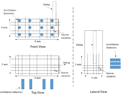
Figure 2-11: Schematic showing the arrangement of scintillation detectors ... 28
Figure 2-12: Scintillation detectors arranged in 3 x 4 matrix in a 2D plane ... 29
xi
Figure 3-1: Experimental setup for runs with liquid injection ... 32
Figure 3-2: Layers and sections in which bed solids were divided ... 34
Figure 3-3: Agglomerates larger than 12500 μm collected from the bottom layer at 0.06 m/s
fluidization gas velocity ... 34
Figure 3-4: Agglomerates larger than 12500 μm collected from the bottom layer on a 12500
µm sieve at 0.60 m/s fluidization gas velocity ... 35
Figure 3-5: Proportion of agglomerates in each layer at Vg = 0.06 m/s at tf = 0 min ... 36
Figure 3-6: Proportion of agglomerates in each layer at Vg = 0.06 m/s at tf = 10 min ... 37
Figure 3-7: Index of Segregation for Bottom and Top layers when the bed was slumped at tf =
0 min at 0.06 m/s gas velocity ... 38
Figure 3-8: Index of Segregation for Bottom layer vs. size of agglomerates at 0.06 m/s
fluidization gas velocity ... 40
Figure 3-9: Index of Segregation for Top layer vs. size of agglomerates at 0.06 m/s fluidization
gas velocity ... 40
Figure 3-10: Index of Segregation for Bottom layer vs. fluidization time at 0.06 m/s fluidization
gas velocity ... 41
Figure 3-11: Index of Segregation for Top layer vs. fluidization time at 0.06 m/s fluidization
gas velocity ... 41
Figure 3-12: Index of Segregation for Bottom layer vs. size of agglomerates at 0.60 m/s
fluidization gas velocity ... 42
Figure 3-13: Index of Segregation for Top layer vs. size of agglomerates at 0.60 m/s
fluidization gas velocity ... 43
Figure 3-14: Lateral distribution of agglomerates for Bottom layer at 0.06 m/s and for a
xii
Figure 3-15: Lateral distribution of agglomerates for Top layer at 0.06 m/s and for a fluidization
time of 2 min ... 45
Figure 3-16: Lateral distribution of agglomerates for Bottom layer at 0.06 m/s and for a
fluidization time of 4 min ... 45
Figure 3-17: Lateral distribution of agglomerates for Top layer at 0.06 m/s and for a fluidization
time of 4 min ... 46
Figure 3-18: Lateral distribution of agglomerates for Bottom layer at 0.06 m/s and for a
fluidization time of 7 min ... 46
Figure 3-19: Lateral distribution of agglomerates for Top layer at 0.06 m/s and for a fluidization
time of 7 min ... 47
Figure 3-20: Lateral distribution of agglomerates for Bottom layer at 0.60 m/s and for a
fluidization time of 0 min ... 47
Figure 3-21: Lateral distribution of agglomerates for Top layer at 0.60 m/s and for a fluidization
time of 0 min ... 48
Figure 3-22: Lateral distribution of agglomerates for Bottom layer at 0.60 m/s and for a
fluidization time of 4 min ... 48
Figure 3-23: Lateral distribution of agglomerates for Top layer at 0.60 m/s and for a fluidization
time of 4 min ... 49
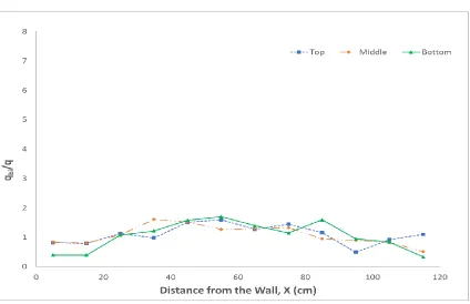
Figure 3-24: Gas bubble profile for Vg = 0.06 m/s (Bottom: h = 12 cm; Middle: h = 32 cm;
Top: h = 52 cm) ... 52
Figure 3-25: Gas bubble profile for Vg = 0.10 m/s (Bottom: h = 12 cm; Middle: h = 32 cm;
Top: h = 52 cm) ... 52
Figure 3-26: Gas bubble profile for Vg = 0.20 m/s (Bottom: h = 12 cm; Middle: h = 32 cm;
xiii
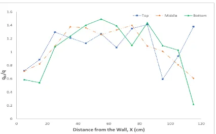
Figure 3-27: Gas bubble profile for Vg = 0.35 m/s (Bottom: h = 12 cm; Middle: h = 32 cm;
Top: h = 52 cm) ... 53
Figure 3-28: Gas bubble profile for Vg = 0.35 m/s with adjusted y-scale (Bottom: h = 12 cm; Middle: h = 32 cm; Top: h = 52 cm) ... 54
Figure 3-29: Gas bubble profile for Vg = 0.50 m/s (Bottom: h = 12 cm; Middle: h = 32 cm; Top: h = 52 cm) ... 54
Figure 3-30: Gas bubble profile for Vg = 0.60 m/s (Bottom: h = 12 cm; Middle: h = 32 cm; Top: h = 52 cm) ... 55
Figure 3-31: Gas bubble profile for Bottom Row for all velocities ... 55
Figure 3-32: Gas bubble profile for Middle Row for all velocities ... 56
Figure 3-33: Gas bubble profile for Top Row for all velocities ... 56
Figure 4-1: Map of 290 source locations for calibration ... 63
Figure 4-2: Error on X for all calibration runs: Predicted values of X vs actual values of X 66 Figure 4-3: Error on Y for all calibration runs: Predicted values of Y vs actual values of Y 66 Figure 4-4: Standard deviation for X-coordinate of location of radioactive particle ... 67
Figure 4-5: Standard deviation for Y-coordinate of location of radioactive particle ... 68
Figure 4-6: Nylon balls of different sizes ... 69
Figure 4-7: Model Agglomerate-1 (MA1) ... 70
Figure 4-8: Tracer locations and gas bubble flow distribution for MA2 at 0.06 m/s and room temperature ... 72
xiv
Figure 4-10: Tracer locations and gas bubble flow distribution for MA2 at 0.35 m/s and room
temperature ... 73
Figure 4-11: Tracer locations and gas bubble flow distribution for MA2 at 0.50 m/s and room
temperature ... 73
Figure 4-12: Tracer locations and gas bubble flow distribution for MA2 at 0.60 m/s and room
temperature ... 74
Figure 4-13: Tracer locations and gas bubble flow distribution for MA2 at 0.06 m/s and 120
℃ ... 74
Figure 4-14: Tracer locations and gas bubble flow distribution for MA2 at 0.35 m/s and 120
℃ ... 75
Figure 4-15: Tracer locations and gas bubble flow distribution for MA2 at 0.60 m/s and 120
℃ ... 75
Figure 4-16: Probability distribution of particle presence for MA2 at 0.06 m/s and room
temperature ... 76
Figure 4-17: Probability distribution of particle presence for MA2 at 0.10 m/s and room
temperature ... 76
Figure 4-18: Probability distribution of particle presence for MA2 at 0.35 m/s and room
temperature ... 77
Figure 4-19: Probability distribution of particle presence for MA2 at 0.50 m/s and room
temperature ... 77
Figure 4-20: Probability distribution of particle presence for MA2 at 0.60 m/s and room
temperature ... 77
Figure 4-21: Probability distribution of MA2 presence at 0.06 m/s and 120 ℃ ... 78
xv
Figure 4-23: Probability distribution of MA2 presence at 0.60 m/s and 120 ℃ ... 78
Figure 4-24: Tracer locations and gas bubble flow distribution for MA1 at 0.06 m/s and room
temperature ... 79
Figure 4-25: Tracer locations and gas bubble flow distribution for MA1 at 0.10 m/s and room
temperature ... 80
Figure 4-26: Tracer locations and gas bubble flow distribution for MA1 at 0.35 m/s and room
temperature ... 80
Figure 4-27: Tracer locations and gas bubble flow distribution for MA1 at 0.50 m/s and room
temperature ... 81
Figure 4-28: Tracer locations and gas bubble flow distribution for MA1 at 0.60 m/s and room
temperature ... 81
Figure 4-29: Tracer locations and gas bubble flow distribution for MA1 at 0.06 m/s and 120
℃ ... 82
Figure 4-30: Tracer locations and gas bubble flow distribution for MA1 at 0.35 m/s and 120
℃ ... 82
Figure 4-31: Tracer locations and gas bubble flow distribution for MA1 at 0.60 m/s and 120
℃ ... 83
Figure 4-32: Probability distribution of particle presence for MA1 at 0.06 m/s and room
temperature ... 84
Figure 4-33: Probability distribution of particle presence for MA1 at 0.10 m/s and room
temperature ... 84
Figure 4-34: Probability distribution of particle presence for MA1 at 0.35 m/s and room
temperature ... 84
Figure 4-35: Probability distribution of particle presence for MA1 at 0.50 m/s and room
xvi
Figure 4-36: Probability distribution of particle presence for MA1 at 0.60 m/s and room
temperature ... 85
Figure 4-37: Probability distribution of MA1 presence at 0.06 m/s and 120 ℃ ... 85
Figure 4-38: Probability distribution of MA1 presence at 0.35 m/s and 120 ℃ ... 86
Figure 4-39: Probability distribution of MA1 presence at 0.60 m/s and 120 ℃ ... 86
Figure 4-40: Index of Segregation for Bottom vs. fluidization time at 0.60 m/s ... 88
Figure 4-41: Index of Segregation for Top vs. fluidization time at 0.60 m/s ... 88
Figure 4-42: Vertical distribution of 12500 µm at 0.60 m/s ... 89
Figure 4-43: Vertical distribution of 5500 µm at 0.60 m/s ... 89
Figure 4-44: Lateral distribution of 12500 µm in Bottom layer at 0.60 m/s ... 90
Figure 4-45: Lateral distribution of 5500 µm in Bottom layer at 0.60 m/s ... 91
Figure 4-46: Lateral distribution of 12500 µm in Top layer at 0.60 m/s ... 91
Figure 4-47: Lateral distribution of 5500 µm in Top layer at 0.60 m/s ... 92
Figure 5-1: Gas bubble profile for Vg = 0.35 m/s in both halves of the fluidized bed (Bottom: h = 12 cm; Middle: h = 32 cm; Top: h = 52 cm) ... 96
Figure 5-2: Gas bubble profile for 0.60 m/s in left and 0.10 m/s in right half of the fluidized bed (Bottom: h = 12 cm; Middle: h = 32 cm; Top: h = 52 cm) ... 96
Figure 5-3: Gas bubble profile for 0.10 m/s in left and 0.60 m/s in right half of the fluidized bed (Bottom: h = 12 cm; Middle: h = 32 cm; Top: h = 52 cm) ... 97
Figure 5-4: Gas bubble profile for Bottom row (h = 12 cm) for all velocities ... 97
Figure 5-5: Gas bubble profile for Middle row (h = 32 cm) for all velocities ... 98
xvii
Figure 5-7: Cumulative mass of all collected agglomerates in the bed ... 100
Figure 5-8: Index of Segregation for the Bottom layer... 100
Figure 5-9: Index of Segregation for the Top layer ... 101
Figure 5-10: Lateral distribution of agglomerates for Bottom layer for 0.35 m/s in both halves of the bed... 102
Figure 5-11: Lateral distribution of agglomerates for Top layer for 0.35 m/s in both halves of the bed ... 102
Figure 5-12: Lateral distribution of agglomerates for Bottom layer for 60L-10R ... 103
Figure 5-13: Lateral distribution of agglomerates for Top layer for 60L-10R ... 103
Figure 5-14: Lateral distribution of agglomerates for Bottom layer for 10L-60R ... 104
Figure 5-15: Lateral distribution of agglomerates for Top layer for 10L-60R ... 104
Figure 5-16: Tracer locations and gas bubble flow distribution for MA2 at 0.35 m/s in both halves of the bed ... 106
Figure 5-17: Tracer locations and gas bubble flow distribution for MA2 at 0.60 m/s in the left and 0.10 m/s in the right side of the bed ... 106
Figure 5-18: Tracer locations and gas bubble flow distribution for MA2 at 0.10 m/s in the left and 0.60 m/s in the right side of the bed ... 107
Figure 5-19: Probability distribution of particle presence for MA2 at 0.35 m/s in both halves of the bed... 107
Figure 5-20: Probability distribution of particle presence for MA2 at 0.60 m/s in the left and 0.10 m/s in the right side of the bed ... 108
xviii
Figure 5-22: Tracer locations and gas bubble flow distribution for MA1 at 0.35 m/s in both
halves of the bed ... 109
Figure 5-23: Tracer locations and gas bubble flow distribution for MA1 at 0.60 m/s in the left
and 0.10 m/s in the right side of the bed ... 109
Figure 5-24: Tracer locations and gas bubble flow distribution for MA1 at 0.10 m/s in the left
and 0.60 m/s in the right side of the bed ... 110
Figure 5-25: Probability distribution of particle presence for MA1 at 0.35 m/s in both halves
of the bed... 110
Figure 5-26: Probability distribution of particle presence for MA1 at 0.60 m/s in the left and
0.10 m/s in the right side of the bed ... 111
Figure 5-27: Probability distribution of particle presence for MA1 at 0.10 m/s in the left and
0.60 m/s in the right side of the bed ... 111
Figure 5-28: Vertical distribution of 12500 µm for the base case (0.35 m/s gas velocity in both
sides of the bed) ... 112
Figure 5-29: Vertical distribution of 12500 µm for the 60L-10R case (0.60 m/s gas velocity in
the left side of the bed and 0.10 m/s in the right side of the bed) ... 113
Figure 5-30: Vertical distribution of 12500 µm for the 10L-60R case (0.10 m/s gas velocity in
the left side of the bed and 0.60 m/s in the right side of the bed) ... 113
Figure 5-31: Vertical distribution of 5500 µm for the base case (0.35 m/s gas velocity in both
sides of the bed) ... 114
Figure 5-32: Vertical distribution of 5500 µm for the 60L-10R case (0.60 m/s gas velocity in
the left side of the bed and 0.10 m/s in the right side of the bed) ... 114
Figure 5-33: Vertical distribution of 5500 µm for the 10L-60R case (0.10 m/s gas velocity in
xix
Figure 5-34: Lateral distribution of 12500 µm in Bottom layer for the base case (0.35 m/s gas
velocity in both sides of the bed) ... 116
Figure 5-35: Lateral distribution of 12500 µm in Bottom layer for the 60L-10R case ... 116
Figure 5-36: Lateral distribution of 12500 µm in Bottom layer for the 10L-60R case ... 117
Figure 5-37: Lateral distribution of 5500 µm in Bottom layer for the base case (0.35 m/s in
both halves of the bed) ... 117
Figure 5-38: Lateral distribution of 5500 µm in Bottom layer for the 60L-10R case ... 118
Figure 5-39: Lateral distribution of 5500 µm in Bottom layer for the 10L-60R case ... 118
Figure A-1: Calibration curves for different combinations of sonic nozzles to supply
fluidization gas to the right side of the bed ... 129
Figure A-2: Calibration curves for different combinations of sonic nozzles to supply
xx
List of Appendices
xxi
Nomenclature
Ao Initial activity of radioactive source (nuclei/s)
AD Activity of source after t seconds (nuclei/s)
t time elapsed (s)
h half-life (s)
I Intensity of radiation (W/m2)
r distance between source and detector (m)
As Activity of source before attenuation (nuclei/s)
ω Mass attenuation coefficient (m2/kg)
ρi Density of medium (kg/m3)
Li Length of medium (m)
x coordinate x from tracer particle (m)
xi coordinate x from detector i (m)
y coordinate y from tracer particle (m)
yi coordinate y from detector i (m)
z coordinate z from tracer particle (m)
zi coordinate z from detector i (m)
Vg Fluidization gas velocity (m/s)
daggl. Size of agglomerate (µm)
xxii
tf Fluidization time (min)
qb Bubbles gas flux (m/s)
qbi Local bubbles gas flux (m/s)
ΔPgrid Gas distributor grid pressure drop (kPa)
Chapter 1
1
Introduction
Canada has the largest bitumen reserves in the world that are extracted from oil sands. Fluid
CokersTM are an essential part of upgrading facilities to produce synthetic crude oil by
thermal cracking of bitumen, which can be pumped through pipelines and processed in oil
refineries. Agglomerates, which consist of particles bound together by liquid, are formed
when bitumen is injected in Fluid CokersTM. When wet agglomerates reach the stripper
region, they bring wet/sticky coke and vapor. The coke depositing on sheds in the stripper
section (lower section of Fluid CokerTM) results in reduction in open area for solids
circulation which eventually leads to de-fluidized zones that causes stripper fouling. Sheds
fouling in the stripper section can lead to premature shutdown of the unit.
The aim of the research work presented in this thesis is to describe the behavior of
agglomerates to develop a better understanding of how bed hydrodynamics and
agglomerate properties affect the motion of agglomerates in a fluidized bed in the context
of Fluid CokingTM technology. However, this work is applicable to other processes as well
which utilize fluidized beds. This chapter introduces key concepts and literature
background related to the research work.
1.1
Bitumen
Bitumen is a type of heavy crude oil that has a viscosity > 1000cP and an API gravity <10o
(Hein, 2017). It is extracted from oil sands in Alberta, Canada. Complex long-chain
hydrocarbon (HC) molecules make up a large fraction of bitumen which need to be broken
to produce lighter, higher-value products.
The vast resources of bitumen in oil sands in Western Canada require extensive processing
to produce transportation fuels. The fraction of vacuum residue in bitumen is 50-60 wt %.
Coking is one of the key technologies for processing vacuum residue, which is converted
1.2
Coking
Coking is a continuous thermal cracking process for the conversion of heavy hydrocarbons
into synthetic crude oil. It produces coke and gases as by-products. Numerous processes
have been developed to thermally crack bituminous materials including visbreaking,
delayed coking, Fluid CokingTM and FlexicokingTM (Javier Sanchez, 2013). Fluid
CokingTM is of particular interest in context of the research work presented in this thesis.
1.3
Fluid Coking
Fluid CokingTM is an upgrading process in which bitumen is injected via spray nozzles into
a fluidized bed of heated coke particles to thermally crack it into more valuable lighter
hydrocarbon products. Preheated feed at 350 ℃ is injected into the fluidized bed of coke
at 500 ℃ to 550 ℃ through steam atomization spray nozzles. The bed temperature should
be maintained such that production of low-value permanent gases by over-cracking is
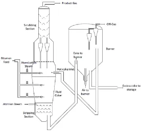
avoided. Figure 1-1 shows a schematic of a Fluid CokerTM.
When feedstock is injected in a downward-flowing bed of hot coke particles, it heats up
and cracks into smaller vapor molecules. Vapors move upward through the bed while the
particles move down to stripper region where valuable vapor product trapped between the
coke particles is recovered through steam stripping. The stripper is equipped with sheds
(baffles) to enhance the removal of hydrocarbon vapors from fluidized coke particles. The
down-moving coke particles are then conveyed to a burner where partial combustion is
used to reheat the coke particles and recirculate them back to the reactor. This provides the
heat required for the endothermic thermal cracking process. Excess coke particles are then
removed, quenched and stockpiled.
The hydrocarbon feed is dispersed into very fine droplets when sprayed into the fluidized
bed which significantly enhances the phase contact area in the reactor and provides a proper
cracking environment for the bitumen feed, without major heat and mass transfer
limitations. The even distribution of droplets improves the heat transfer, for a rapid and
effective process (Base et al., 1999).
Gray et al. (2003) mentioned that the time required for Athabasca bitumen to completely
react is around 24 s at 503 °C. Furthermore, the adhesive forces caused by reacting material
are only significant when the film is still liquid and capable to form liquid bridges between
coke particles. Particles can grow either by normal growth by laying down product coke
on the individual particles or by coke-particles agglomerating.
The stripper displaces hydrocarbons in the interstitial voids between the coke particles by
using countercurrent contact with steam. Stripping is most effective in a dense, moving
fluidized bed. When the steam is injected at the bottom of the stripper, bubbles rise opposite
to the down-flowing coke stream entering from the top (Wiens, 2010). To enhance the
contact between steam and the coke particles, baffles known as “shed decks” or simply
sheds, are employed in the stripping section of the reactor (Blaser et al., 1986; Graf &
1.3.1
Fouling
One of the most common issues encountered in Fluid CokingTM is fouling of the stripper
section of the reactor because of solid coke deposits. The build-up of undesirable material
on the surfaces of process equipment is usually referred to as fouling. The rate of fouling
can be defined by the change of rate of deposition and the rate of removal. When fouling
arises in a process, there are two likely scenarios that can occur:
1. The deposition rate is always greater than the removal rate and a complete barrier
to the flow will be formed after some time
2. Equilibrium will be reached after a certain period when the removal rate is equal
to the deposition rate
In a Fluid CokerTM, the deposition rate is always greater than the removal rate and a
complete barrier to the flow is eventually formed. Fouling impacts negatively on yield and
throughput of the unit, and reduces the total run-time between shutdowns.
1.3.2
Sheds
Fluidization can be improved by breaking and re-distributing the bubbles by using internals
(Javier Sanchez, 2013) such as baffles, especially with Group B powders (Geldart, 1973).
Bubble size plays an important role for gas/solid mass transfer in bubbling fluidized beds.
The coke particles in the wake around the bubbles interact with the gas inside the bubbles
resulting in mass transfer between gas and solid. This mass transfer can be improved by
decreasing the bubble size and renewing the wake around the bubble by exchanging the
gas components from the emulsion phase (Yang, 2003).
A schematic diagram of a small section of sheds in the stripper section in a Fluid CokerTM
is shown in Figure 1-2. The open area for solids circulation reduces when coke particles
Figure 1-2: Fouling caused by unwanted coke deposition on the sheds and walls of the Fluid CokerTM stripper section (Adopted from Bi et al., 2005)
Coke gradually deposits on the surface of the sheds. When the coke gathered on the middle
row reaches the top row of the sheds, the flow of coke particles is increasingly restricted
until the shutdown of the Fluid CokerTM for cleaning becomes unavoidable. To avoid the
premature shutdown of the unit, it is very important that coke deposits on the sheds is
minimized.
1.4
Agglomeration
The phenomenon of particles sticking to each other is called agglomeration. In some
processes, agglomeration is desirable such as in pharmaceuticals and fertilizer industries
where dustiness can be reduced by agglomeration (Weber, 2009). However, in processes
such as Fluid CokingTM, agglomeration is highly undesirable as it reduces the production
yield when agglomerates with considerable amount of high value unreacted hydrocarbons
leave the Coker to be burned in the burner. In Fluid CokersTM, agglomeration causes both
mass transfer and heat transfer limitations. Mass transfer limitations prevent the cracked
products from moving to the vapor phase in the bed resulting in the formation of coke,
accumulation in the bed and further agglomeration which increases the risk of bogging and
de-fluidization (House, 2007). Agglomeration also causes fouling of the internals and
surfaces such as sheds/baffles (Javier Sanchez, 2013).
1.4.1
Formation of Agglomerates
When liquid is injected in a fluidized bed, it does not vaporize instantaneously even if the
bed is operated above the boiling point of the liquid. Agglomerates are almost immediately
formed when particles and liquid jet come in contact. These agglomerates then move
around the rest of the fluidized bed.
Ariyapadi et al. (2003) studied the agglomerate formation using X-ray imaging. An opaque
radio liquid tracer with ethanol was injected to visualize the jet cavity. It was observed that
agglomerates formed because of coalescence of liquid droplets and solid particles at the
end of the jet cavity.
A study by Schaefer & Mathiesen (1996) showed that there are two mechanisms by which
initial contact between liquid droplets and particles occur,
1. When droplets are small, wetting is caused by the distribution of droplets on
individual solid particulates. This leads to coalescence between wet solid particles.
2. When droplets are large, wetting is caused by the immersion of large number of
solid particles in the liquid.
House (2007) showed using open air experiments that the first mechanism occurs in Fluid
CokersTM. The results showed that the Sauter mean diameter of the liquid droplets is
equivalent to the Sauter mean diameter of the coke particles, hence, leading to the result
that the first mechanism is prevalent in Fluid CokerTM.
For agglomeration to occur, the viscosity of the liquid and contact angle are two key factors
that are independent of fluidization gas velocity (McDougall et al., 2005). A low contact
angle between the liquid and solid surface results in well wetted particles. When the
high viscosity. However, when the contact angle is high, agglomerate formation will
always take place (McDougall et al., 2005).
1.5
Models for the Study of Agglomerate Formation
Several experimental models are available to generate agglomerates by liquid injection in
a fluidized bed under conditions that simulate agglomerate formation in Fluid CokersTM.
Such models include the PlexiglasTM experimental model developed by Morales (2013)
and the Gum Arabic model developed by Reyes (2015). Both models produce an
agglomerate distribution that matches the agglomerate distribution obtained in a pilot plant
Fluid CokerTM (Reyes, 2015).
The model developed by Morales (2013) uses Plexiglas as a binder dissolved in a mixture
of acetone and pentane, and sand as fluidized solids. Since the acetone-pentane mixture
can form combustible mixtures with air or in some cases explosive mixtures, nitrogen had
to be used as fluidization gas for this model which is quite expensive compared to air. The
experiments were conducted at 68 ℃. The experimental technique also required a complex
procedure to measure the initial concentration of liquid in agglomerates (Soxhlet
extraction) that caused the measurements to be conducted on small proportions of the
agglomerates. The flammable and toxic acetone and pentane also posed health and
environmental hazards.
The advantages of the Gum Arabic model developed by Reyes (2015) is that it can be
operated at 120 ℃ and while it provides a similar distribution of agglomerates formed, is
more flexible in terms of operation, control and complexity as it does not form explosive
mixtures with air and does not need a complex procedure to determine the initial liquid
content of the recovered agglomerates. The binder solution for the model developed by
Reyes (2015) requires a mixture of Gum Arabic (as binder), food dye (tracer) and water
(solvent) that causes no environmental or health impact. Also, the measurement procedure
to estimate concentration of the binder in the solution is accurate thanks to the use of food
dye. For this reason, the Gum Arabic model was used for agglomerates formation by liquid
as the solvent. Water wets sand particles well as bitumen wets coke particles in Fluid
CokersTM (Prociw, 2014).
In either case, agglomerates were generated by injecting the binder solution into the
fluidized bed. The agglomerates were then collected and analyzed to determine the size
distribution and the initial binder concentration.
1.6
Tribo-Electric Method for Bubble Flow Distribution
The particles in a fluidized bed move when bubbles of fluidization gas move through the
bed. The local gas bubble flux varies greatly over the bed cross-section. The motion of
agglomerates is also affected by the distribution of gas bubble flux.
Various methodologies have been developed by scientists to visualize or quantify the
bubble flow distribution. Some of the methodologies include direct visualization using
image analysis, X-ray image analysis, X-ray tomography, optical probes etc. Jahanmiri
(2017), developed a novel tribo-electric method to quantify the gas bubbles distribution in
a fluidized bed.
1.6.1
Theory and Background
Some materials become electrically charged after a frictional contact with another material.
This phenomenon is known as the triboelectric effect. Jahanmiri (2017) showed that in a
fluidized bed, triboelectric probes can be used reliably to determine the fluidization gas
bubble flow distribution. The triboelectric probes generate electric current when solids in
the wake of the bubbles interact with the triboelectric probe. This electric signal enables us
to determine the local bubble flux from the characteristics of the signals, i.e. power and
average frequency, obtained from a triboelectric probe. The signals can be analyzed using
a data analysis tool such as power spectrum.
For the research work presented here, an array of 12 x 3 triboelectric rods was used to
determine the fluidization gas bubble flow distribution in the fluidized bed (Figure 2-5).
The advantage of triboelectric rods over optical or conductance probes is that triboelectric
velocities such as 1 m/s without bending or breaking. They also require minimal
maintenance.
1.7
Radioactive Particle Tracking
Radioactive Particle Tracking (RPT) is a non-intrusive technique to track the motion of a
single radioactive particle (source) in a vessel without disrupting the flow inside (Shehata
et al., 2007). The concept was first developed by Kondukov in 1965. However, Lin et al.
(1985) were the first to successfully attain their objectives to study the motion of solids
inside a fluidized bed and observe a change in direction of solids motion as the gas velocity
was increased. Moslemian et al. (1992) then made data sampling faster and easier by
introducing digital pulse counters. RPT has been improved significantly since its
conception by various scientists and several new applications have been found for this
method (Ayatollahi, 2016).
1.7.1
Theory and Background
RPT works on the principle that a radioactive particle releases γ-rays. These γ-rays can be
detected using scintillation detectors and, hence, the distance can be measured from the
source as a function of radiation strength. Based on the distances from different scintillation
detectors, location coordinates of the radioactive source in a fluidized bed can be
determined. Scintillation detectors should be placed around the controlled volume in such
a way that they provide sufficient redundancy to calculate the location of the tracer particle.
Radioactive nuclei can emit alpha, beta and gamma radiations. The selection of scintillation
material depends on the type of radiation to be detected and the type of radiation to be
detected is determined by the radioactive isotope used. For example, a NaI scintillation
detector is used to detect gamma radiation whereas a ZnS scintillation detector can be used
to detect alpha radiation. Each type of radiation has a different penetration capability (alpha
with the lowest and gamma with the highest), therefore, the selection of radio-isotope
depends on the system that needs to be observed. In this case, the highest penetrating
radiation was needed i.e. gamma rays. Hence, the radio-isotope and the detection system
1.7.2
Factors Affecting Strength of Radioactive Source
Several factors affect the strength of the radioactive source including time (half-life),
distance of detector from the source and mass attenuation due to media present between
the detector and the source etc. Hence, a correction is required for each factor when
calculating the intensity of radiation.
1.7.2.1
Half Life
The number of parent nuclei of radioisotope decreases when they undergo disintegration
and release nuclear radiation. The time elapsed, while the number of parent nuclei reduce
to half of the initial value, is called half-life. For example, the half-life of Scandium-46 is
83.79 days which means approximately 50 of the 100 initial parent nuclei will be left after
83.79 days and so on. Reduction in number of parent nuclei reduces the activity of the
radioactive source (number of radioactive disintegrations per second) in the same
proportion. Equation (1.1) represents the correlation to determine the radioactivity of a
source after any given time.
𝐴𝐷 = 𝐴𝑜∙ (1 2⁄ )
𝑡 ℎ ⁄
(1.1)
In this equation, h is the half-life of the radioactive material.
1.7.2.2
Effect of Distance on Radiation Strength
The radiation strength reduces as the source moves away from the detector. (Javier
Sanchez, 2013) The effect of distance on radiation strength can be determined by the
Inverse Square Law as given by Equation (1.2).
𝐼 ∝ 1
𝑟2 (1.2)
1.7.2.3
Attenuation
The radiation emitted from radioactive source loses its intensity when it passes through a
medium or a series of media due to interaction between radiation and the medium it passes
medium is characteristic of the type of medium (i.e. mass attenuation coefficient) and its
length (Ayatollahi, 2016). The absorption of radiation in a series of different media can be
determined using the generalized Beer-Lambert law in Equation (1.3) which gives the
radioactivity corrected for the attenuation.
𝐴𝐷 = 𝐴𝑠 ∙ exp(− ∑ 𝜔𝑖 𝑖𝜌𝑖𝐿𝑖) (1.3)
The energy of gamma rays emitted by the source should be high enough so that it can be
detected by the detector after attenuation through the system.
1.7.3
Working Principle of Scintillation Detectors
A scintillator is a material which, when struck by an incoming radiation source, absorbs
the energy of the incoming radiation. The absorbed energy is re-emitted by the scintillator
as a photon of visible light after a certain decay time. Decay time can vary from a few
nanoseconds to several hours depending on the material of the scintillator. In this case, a
scintillator with a very small decay time was needed to create an RPT system with a
considerable short sampling time.
By coupling a scintillator to an electronic light sensor, such as photomultiplier (PMT), a
scintillation detector is obtained. When a PMT absorbs a photon, it re-emits the energy as
an electric pulse due to photoelectric effect. Hence, a scintillation detector counts the
incident radiations in two steps. In the first step, a photon is generated by the scintillator
when the scintillator is struck by a radiation source. In the second step, this photon goes to
the PMT and strikes a thin metal foil, also known as photocathode, causing an electron to
eject from the photocathode. The ejected electron is electrostatically accelerated to a high
energy and strikes a series of metal cups which are located just past the photocathode. This
successive collision with metal cups generates secondary electrons resulting in an
amplified electric pulse in the end which can be measured by the electronic circuit. The
intensity of the radiation can be determined by measuring the number of electric pulses
generated per unit time.
The external photons can affect the ionization events caused by incident radiation if the
mylar, is often used to shield the scintillator. However, the foil thickness should be selected
in a way that it minimizes the attenuation of the incident radiation.
1.7.3.1
Calibration of Scintillation Detectors
The effect of distance on the strength of radiation source can be corrected if the distance
between the source and detector is known. The coordinates of the detector are known as
the detector has a fixed known location, but the location coordinates of a radioactive
particle are not known when the RPT system is used to track the motion of a particle. It
means the distance between the source and detector is unknown and correction due to
strength cannot be known. Calibration of scintillation detectors is carried out to eliminate
this problem. A calibration curve is generated by placing the radioactive source at several
known locations and measuring the intensity of radiation from the source (Javier Sanchez,
2013).
Figure 1-3 shows an example of a calibration curve which provides distance between the
center of detector and radioactive particle as a function of normalized radiation data. It is
clear from the calibration curve that the closer the particle, the higher the intensity of the
radiation. Hence, distance can be obtained from the above curve, if radiation data from the
detector is available. For more information on calibration, please refer to Chapter 4
(Section 4.1.1).
1.7.4
Rendition Techniques
Several rendition techniques can be used to obtain the location coordinates of a radioactive
source as a function of time in a fluidized bed. The most common methods used are,
1. Computer Aided Radioactive Particle Tracking (CARPT)
2. Monte Carlo Simulation
1.7.4.1
Computer Aided Radioactive Particle Tracking (CARPT)
This method was first introduced by Lin et al. (1985). Before the position of tracer can be
determined, an in-situ calibration must be conducted by placing the tracer at several known
positions and measuring the radiation intensity by each detector. A calibration curve is
established for each detector from the obtained information to correlate the intensity
measured by the detector to the distance between the tracer and the center of the detector
surface. The calibration curve can have different shape and order. The calibration curve
usually is developed by curve fitting of the raw data and the fitted curve. Several
polynomial fits of different orders are used to determine the relationship of distance versus
γ-rays counts (Chaouki et al., 1997).
The distance between the ith detector (xi, yi, zi) and the source (x, y, z) can be measured
using the two-points distance formula given in Equation (1.4).
𝑟𝑖2 = (𝑥 − 𝑥𝑖)2+ (𝑦 − 𝑦𝑖)2+ (𝑧 − 𝑧𝑖)2 (1.4)
Where r is the distance that is attained from the polynomial fitting. Since the data is
location determination. Lin et al. (1985) used a weighted least-square exact linearization
method to take advantage of the available redundancy.
The main advantages of the CARPT method are simplicity of the mathematics and less
amount of processing time required. The disadvantages of this method are that it needs an
extensive calibration and still the model does not consider the angle between the tracer and
a horizontal axis through the center of the scintillation detector.
1.7.4.2
Monte Carlo Rendition Technique
This method was developed by Dr. Chaouki and his group at École Polytechnique de
Montréal. This method takes into account both the geometry and effect of radiations in
RPT. This eliminates the need for the extensive in-situ calibration, but increases the
computer processing time. The determination of the tracer location from the detectors
counts involves the development of a map of counts as a function of the possible
coordinates of the source. Since a certain fraction of the γ-rays are absorbed by the fluidized
material and by the vessel walls, a new map is needed whenever the density of the medium
to be studied changes (Chaouki et al., 1997).
The unfortunate disadvantage of using this method is that it requires high computation time
due to complex mathematics. One coordinate per second is the approximate rate to obtain
the position. It means it will take around 11 days to calculate coordinates from the data if
one million data points are present in the data. This would take 5 minutes when CARPT
method is used (Javier Sanchez, 2013).
1.8
Research Objectives and Outline
The main objective of the research work conducted in this thesis is to develop a better
understanding of how agglomerates move through a fluidized bed, and how their motion
is affected by bed hydrodynamics. To achieve this target, model agglomerates were
manufactured with a radioactive source so that they can be tracked when they move in the
fluidized bed unit. But before model agglomerates could be manufactured, the properties
of such agglomerates needed to be determined in a separate set of experiments. Hence, the
Chapter-3: A preliminary study was conducted to determine which agglomerates segregate in a fluidized bed and their properties such as size and density. Preliminary
experiments were conducted by injecting a binder liquid solution of Gum Arabic (GA) in
a fluidized bed of sand and air. The cold model developed by Reyes (2015) was adopted
for these experiments, as Reyes (2015) showed that the GA model gives an agglomerate
distribution similar to that of a pilot Fluid CokerTM. The agglomerates produced in these
experiments were collected and their properties were determined. Agglomerates that
segregated were also identified in these experiments. Gas bubble flow distribution was also
measured using the tribo-electric method to study the impact of bubbles distribution on
segregation.
Chapter-4: This chapter describes the development of new method for a 2D RPT system. Initially, CARPT method was used to determine the location coordinates of a radioactive
model agglomerate in a fluidized bed, but it did not work because all the detectors were in
a 2D plane for the RPT setup. CARPT method is applicable for a system with detectors in
a 3D plane. After the development of the new method, the motion of model agglomerates
was investigated for various velocities at room temperature and 120 ℃. The size of model
agglomerates was based on the properties of actual agglomerates that were found important
in the preliminary studies (Chapter-3).
Chapter-5: After successful implementation of the new method for our 2D RPT system, experiments were conducted with split gas velocities. It was achieved by creating two
different gas velocities in two halves of the bed as fluidization air can be supplied to both
halves independently. The purpose of this investigation was to determine how
agglomerates behave when one half of the bed has a higher gas velocity or more gas
bubbles, which simulates the core-annular flow observed in Fluid CokersTM. Experiments
were also conducted with the GA model, to obtain preliminary segregation results and
agglomerate properties to compare with the experiments with same gas velocities in both
halves of the fluidized bed, and the tribo-electric method was used to measure the gas
Chapter 2
2
Experimental Setup and Methodology
This chapter describes the equipment setup used for all the experiments. It describes the
methodologies used for the experiments conducted as well, but each chapter will also
provide experimental procedures specific to those chapters.
2.1
Equipment
For all experiments, the same equipment was used for the fluidized bed. However, some
minor changes were made in the equipment during the research work. A schematic diagram
of the equipment with its dimensions is presented in Figure 2-1.
Fluidization Gas (Vg)
Fluidization Gas (Vg)
Gas Distributor (2 Sections)
Front View Lateral View
0.40 m
2.3 m 1.2 m
0.15 m 1.5 m 0.47 m
Initial Bed Mass: Sand
150 Kg (ρ: 2650 kg/m3) Dipleg
Dipleg
The equipment used was 2.3 m high with a cross section of 1.2 m by 0.15 m. It had an
expansion zone of cross sectional area of 1.2 m by 0.47 m at the height of 1.5 m.
Fluidization gas was provided by two independent gas distributors. The mass flow of
fluidization gas to the gas distributors could be controlled independently using two banks
of sonic nozzles, one for each distributor. It was also equipped with one primary cyclone
and one secondary cyclone. The dipleg from the primary cyclone recycled the collected
particles back to the bed.
2.2
Fluidized Bed
Silica sand with a Sauter mean diameter of 190 µm and a particle density of 2650 kg/m3
was used as fluidized solids. For all experiments, 150 kg of silica sand was used making a
fixed bed with a height of 0.54 m. Figure 2-2 shows the particle size distribution for the
silica sand used in this study.
Air was used as fluidization gas which was provided by the two gas distributors. The air
flow was controlled by the two banks of sonic nozzles upstream of the fluidization gas
distributors as shown in Figure 2-3. Air was used as fluidization gas as it is compatible
with the binder liquid solution injected for agglomerates formation. The calculated
minimum fluidization velocity for this system is 0.04 m/s.
Inlet PCV PG LHSB-S LHSB-M LHSB-L RHSB-S RHSB-M RHSB-L BV BV BV BV BV BV PG PSV PG PSV To Bed To Bed LEGEND:
Pressure Control Valve: PCV Pressure Gauge: PG Isolation Ball Valve: BV Left Hand Sonic Bank: LHSB Right Hand Sonic Bank: RHSB Small, Medium, Large: S, M, L Pressure Safety Valve: PSV
Figure 2-3: Sonic nozzle banks upstream of gas distributors which provide the fluidization air
Before experiments were conducted, the sonic nozzle banks were calibrated to obtain the
data of mass flow rates for the given upstream operating pressures. The detailed operating
and calculation procedure is provided as Appendix A.
2.3
Liquid Injection System
The liquid binder solution was injected at constant flowrate from a blow tank, pressurized
with nitrogen, into the fluidized bed. A spray nozzle, with exit diameter of 2.7 mm, that
used nitrogen gas to atomize the liquid into small droplets was used to inject the liquid in
Conditioner (BFC) pre-mixer was used to mix the atomizing nitrogen gas and liquid binder
solution upstream of the spray nozzle. The liquid solution was mixed with the atomizing
gas at an angle of 30⁰ as shown in Figure 2-5.
Figure 2-4: Liquid injection system
Figure 2-5: Bilateral Flow Conditioner (BFC) pre-mixer
Open air experiments were conducted to adjust all the pressure transducers such that the
liquid injection system injects 30 g/s of liquid binder solution with a Gas to Liquid Ratio
(GLR) of 2 wt%.
2.4
Agglomerates Recovery
Once an experimental run had been completed and the bed had been de-fluidized and
cooled, the agglomerates were collected by sieving the bed mass as established by Morales
(2013). The total bed mass recovered is categorized into three groups: macro-agglomerates
(≥ 600 µm), micro-agglomerates (< 600 µm) and individual solid bed particles. Since there
macro-agglomerates were, therefore, obtained by sieving the mass of all bed solids.
Macro-agglomerates were then sieved into following size cuts:
daggl ≥ 12500 µm
12500 µm > daggl ≥ 9500 µm
9500 µm > daggl ≥ 4750 µm
4750 µm > daggl ≥ 4000 µm
4000 µm > daggl ≥ 2000 µm
2000 µm > daggl ≥ 1400 µm
1400 µm > daggl ≥ 850 µm
850 µm > daggl ≥ 600 µm
Because individual particles smaller than 600 µm were also present in the bed, retrieval of
just micro-agglomerates free of individual particles was not possible. Therefore, the
quantity and properties of micro-agglomerates were estimated from a representative
sample that was taken after macro-agglomerates were recovered. The representative
sample was then sieved to collect following size cuts:
600 µm > dp ≥ 500 µm
500 µm > dp ≥ 425 µm
425 µm > dp ≥ 355 µm
In this thesis, each size cut is identified by its smallest value. For example, agglomerates
of the size cut 425 µm > dp ≥ 355 µm are recognized as agglomerates of size 355 µm.
2.5
Agglomerates Analysis
The mass and density of macro-agglomerates were determined for each size cut after
sieving. The procedure of estimation of mass and liquid to solid ratio (L/S) for
micro-agglomerates is very well described by Reyes (2015). In summary, it consists of the
following steps:
2. Estimation of dye (tracer) in the micro-agglomerates using UV – spectroscopy
(helped determining the L/S for both macro and micro-agglomerates)
3. Determination of mass of fine particles in agglomerates with the help of laser
diffraction method
It was observed during preliminary studies that micro agglomerates did not segregate,
therefore, micro-agglomerates were not analyzed for all later experiments.
2.6
Tribo-Electric Method
A total of 36 triboelectric rods were used to measure the gas bubble flow at 36 locations in
the fluidized bed at the same time (Figure 2-6). The rods were inserted halfway into the
bed to measure the time-averaged gas bubble flow. As the rods were inserted half way in
the bed, they measured the tribo-electricity generated over the length of the rod that was
inside the bed. Since 12 rods are placed in one row to measure the lateral bubbles
distribution, the radial direction in which one rod is inserted is not important (later radial
dimension or z-axis was also ignored for Radioactive Particle Tracking or RPT). This
approach is different than the strategy used by Jahanmiri (2017). He inserted and moved
the rod (covered with tygon coating exposing only 12 mm tip to measure local bubble flux)
in the lateral direction to measure the local bubble flow at various locations. In our case,
placing the 12 rods eliminated the need of moving the rods in any direction and enabled to
obtain the 12 measurements in one row at the same time.
One of the triboelectric rods used is shown in Figure 2-7. The electric current generated by
the triboelectric rods was then converted to voltage and amplified by a multirange amplifier
which converted an input of 0-200 nA to an output of 0-10.4 V. The amplifier was linked
to a data acquisition system that recorded the amplified signal every millisecond (sampling
time of 1 ms) for 300 seconds. The experiments were conducted at room temperature for
Gas Distributor (2 Sections)
Front View Lateral View
Top Row: z = 52 cm
2.3 m 1.2 m
0.15 m 1.5 m 0.47 m
Tribo-electric rods
(Tribo-probes) Tribo-electric rods
Middle Row: z = 32 cm
Bottom Row: z = 12 cm
Figure 2-6: Array of triboelectric rods comprised of 3 rows and 12 columns inserted half way in the fluidized bed
2.6.1 Analysis of Triboelectric Signals
Jahanmiri (2017) showed that the best results for signal analysis were obtained when a
correlation for gas bubble flux based on two variables was used by combining the power
and average frequency, hence, the power spectrum of a signal. The average frequency and
power of the signals can be calculated by the Equations (2.1) and (2.2), where f is the
frequency and P(f).df is the power between the frequencies (f-df/2) and (f+df/2), as
determined with the Fast Fourier Transform:
𝐴𝑣𝑒𝑟𝑎𝑔𝑒 𝐹𝑟𝑒𝑞𝑢𝑒𝑛𝑐𝑦 (𝑓𝑎𝑣𝑔.) =
∫025𝑃(𝑓).𝑓.𝑑𝑓
∫025𝑃(𝑓).𝑑𝑓 (2.1)
𝐴𝑣𝑒𝑟𝑎𝑔𝑒 𝑃𝑜𝑤𝑒𝑟 (𝑃) = 1
25∫ 𝑃(𝑓). 𝑑𝑓 25
0 (2.2)
The local gas bubble flux (qbi) can be calculated using the average frequency (fi) and power
(Pi) obtained from the above equations, using the Equation (2.3):
𝑞𝑏𝑖 = 𝑎. 𝑃𝑖𝑏. 𝑓𝑖𝑐 (2.3)
The values of a, b and c were determined for the obtained data for each flowrate by
minimizing the error between the experimental values and measured values as explained
by Jahanmiri (2017).
2.7
Radioactive Particle Tracking (RPT) System
As described in Section 1.7, the development of the Radioactive Particle Tracking (RPT)
system will depend on the type of radiation suitable for the intended application. In this
case, the equipment wall was made of quarter inch iron sheet with a fluidized bed of silica
sand inside. Therefore, alpha and beta radiations would not be able to penetrate the
fluidized bed of sand and the equipment wall because of attenuation in radiation strength
of the radioactive source. Hence, a radioactive source (further termed as source) with
gamma decay was needed to make the RPT system work because of the non-disruptive
2.7.1 Radioactive Particle/Source
Before actual experiments could be performed, calibration of the system was required by
placing the particle inside the fluidized bed at known locations and recording the radiation
strength for each location. It was estimated that it would take more than 3 months to
complete the calibration of the system, therefore, a radioactive source with significant
half-life was needed which would be environmental friendly as well. For this reason,
Scandium-46 (Sc-Scandium-46) isotope with a half-life of 83.79 days was chosen. Another advantage of Sc-Scandium-46
is that it disintegrates into Titanium-46 (Ti-46) which does not pose any environmental or
biological hazards.
The decay scheme of Sc-46 into Ti-46 is given in Figure 2-8.
Figure 2-8: Decay scheme of Sc-46
2.7.2 Scintillation Detectors
Scintillation detectors consist of a scintillator and a photomultiplier (PMT). Selection of a
a scintillation detector with the capability of detecting gamma rays was required. For
selection of a scintillation detector, the decay time is very important as it defines the
minimum sampling time for the system (This decay time is not the same as half-life or
radioactive decay. Please refer to Section 1.7.3 for further information). For this system, a
scintillation detector with minimum decay time was required.
Sodium Iodide with activated Thallium [NaI(Tl)] is a commonly used scintillator with a
decay time of only 0.23 µs which was highly desirable for this work. The scintillation
detector used to obtain intensities of gamma rays for the research work presented in this
thesis was 2M2/2 (Saint-Gobain Crystals, USA). The cylindrical NaI scintillator was of 2”
x 2” size with 0.2% thallium (Tl) impurity as activator. Thallium in the crystal structure of
NaI converted the energy absorbed in the crystal by the radiation into visible light. The
visible light generated by thallium was then converted and amplified by an integrally
Figure 2-9: NaI(Tl) scintillation crystal used for the current research work (Saint-Gobain Crystals Inc.)
The NaI scintillation detector was coupled with an ORTEC digiBASE (Figure 2-10)
externally which was used for data acquisition and processing through CONNECTION-32
and MAESTRO®-32 programs. This base consisted of a preamplifier and a powerful
Figure 2-10: Scintillation detector mounted on data acquisition (DAQ) base
Each scintillation detector was connected to a computer (also called Client computer) via
a USB cable. The client computer measured the detector signal every 6 ms using a program
on LabWindows CVI (National Instruments, Austin, TX) platform. This program was
developed by Javier Sanchez (2013). Sanchez also found that by placing a USB hub
between each detector and client computer speeds up data transmission from digiBase to
client computer which reduced the sampling time from 62 ms to 6 ms.
2.7.3 Experimental Setup
The current RPT system at the Institute for Chemicals and Fuels from Alternative
Resources (ICFAR) includes:
• A single radioactive source (Sc-46) emitting γ-rays
• 12 scintillation detectors arranged in a 2D plane to count the radiations emitted
• One computer for each scintillation detector along with a master computer to