Tracking Unknown Number of Stealth Targets in a Multi-Static
Radar with Unknown Receiver Detection Profile Using RCS Model
Amin Razmi1, Mohammad A. Masnadi-Shirazi2, *, and Alireza Masnadi-Shirazi1
Abstract—The reliable detection of geometrically-based stealth targets using a conventional single sensor radar system may be extremely difficult. This is because low Radar Cross Section (RCS) from certain angles results in a low Signal to Noise Ratio (SNR). In the present work, multi-target tracking of stealth targets is investigated in a multi-static radar with passive receivers. The Directions of Arrival (DOA) of targets are estimated by the receivers without knowing the number of targets, and their positions are obtained based on the transmitter beam direction. The B2 bomber aircraft model has been used as a stealth target. The RCS of the model has been simulated for all collection of incident and reflected angles from an oblique impinging plane wave. Probability of Detection (Pd) is modeled using a Toeplitz-based method for different SNRs due to different RCS patterns and is fed to an Iterated Corrected Probability Hypothesis Density (IC-PHD) filter. In spite of considering the transmitter and receivers resolution in our input data generation, the proposed algorithm is able to track the targets individually when they are much close to or even cross each other. Simulation results show the improved performance of the proposed method compared to other existing approaches.
1. INTRODUCTION
Multi-target tracking techniques along with sensing and computing technologies have been a center of research attention in more than 50 years. The corresponding methods and algorithms are reviewed in many articles [1–3]. Generally speaking, multi-target tracking algorithms fall into three different paradigms: 1) the Joint Probabilistic Data Association Filter (JPDAF) [4], 2) Multiple Hypothesis Tracking (MHT) [5] and 3) Random Finite Set (RFS)-based multi-target filters [6, 7].
Traditional multi-target tracking paradigms like JPDAF and MHT are based on data association algorithms which partition the measurements to false alarms and potential tracks that lead to multiple single-target filtering for estimating the state of targets.
Conventional multi-target filtering approaches typically employ divide and conquer strategies that partition a multi-target problem into a family of parallel single-target problems. RFS-based methods, however, have the advantage of being capable of estimating the multi-target states while avoiding data association complexities [3].
Multi-target tracking incorporating multiple sensors faces four challenges. 1) The number of targets being unknown and time-varying. 2) Detections including clutter (false detections) due to unwanted obstacles or a surge of background noise. 3) Presence of target missed detections due to the sensors being non-ideal and 4) Fusing measurements collected from different sensors in a consistent manner [8]. At each time step, the RFS-based filter propagates the spatial distribution of the sources represented by the first moment approximation of the RFS Bayes filter known as the Probability Hypothesis Density (PHD) [9]. We recall that the PHD filter is a tractable approximation to RFS-based multi-target
Received 18 April 2018, Accepted 28 June 2018, Scheduled 15 July 2018
* Corresponding author: Mohammad Ali Masnadi-Shirazi ([email protected]).
1 Department of Electrical and Computer Engineering, Shiraz University, Shiraz, Iran. 2 School of Electrical and Computer
Bayes filter. Along with the discrete distribution on the number of sources known as the cardinality distribution, different variations of the PHD filter for multi-target tracking are considered, namely, the iterated corrector CPHD filter and general computationally tractable CPHD filter [10–12].
The reliable detection of multiple stealth targets using a conventional single sensor is deemed extremely difficult due to the low Radar Cross Section (RCS) at certain angles might create many missed detections. Consequently, multi-static radar technology has been investigated in such scenarios for detecting and tracking stealth targets [13]. The main advantages over traditional mono-static radars are the improved detection and enhanced clutter rejection due to better target signature. This is due to the diversity of Field of Views (FOV) in a multi-static configuration as geometrically-based stealth technology might make a target act stealthily with respect to a certain FOV but not stealthy with respect to another FOV [14].
In this paper we propose a multi-static radar configuration consisting of one transmitter and multiple passive receivers allocated far apart to create FOV diversity in order to detect the stealthy targets. The targets are illuminated by the single transmitter with its reflection being picked up by the passive receivers. Each passive receiver consists of an antenna array which can perform Direction of Arrival (DOA) estimation. The DOAs of all passive receivers are then fused to effectively triangulate the position of the targets according to intersection of the transmitter beam direction and DOAs while estimating the number of targets and provide measurements for targets.
This paper includes a combination of electromagnetic field, signal processing, data processing and their interactions. Moreover, the aim is to consider real challenges and problems. The stealth aircraft modeling and RCS estimation are analyzed using electromagnetic field approach, while Probability of Detection (Pd), DOA and number of targets estimation in sensors are different parts of signal processing. In addition, the data processing considers multi-sensor multi-target filtering of the detected data in order to eliminate false alarms, generate profiles for newly born targets and filter tracks.
Therefore, the proposed method consists of two stages. In the first stage the RCS pattern of a stealth target is modeled, and a DOA estimation algorithm needs to be implemented for each passive receiver. It is noted that at this stage since the number of targets is unknown, DOA estimation methods like classical MUSIC [15] which assume known number of sources can no longer be used. Instead DOA estimation methods like MUSIC-like [16] and Toeplitz-based [17] that making no assumption on the number of sources can be utilized. Toeplitz-based algorithm is used in the proposed method for estimating DOAs and Pd modeling.
In the second stage, the measurements from all the receivers are then fused together using multi-sensor Iterated Corrected Probability Hypothesis Density filter (IC-PHD) with Pd modeled in the previous part. At each time step, the IC-PHD filter applies the PHD corrector step with the sensors in order. In this way the correction result with sensor data is supposed as the prediction step for the next sensor.
The paper is organized as follows. In Section 2, first of all geometry of the problem including transmitter, receivers and targets relative position is illustrated. In Section 2.1 SNR prediction using RCS evaluation is described. This RCS model is used for SNR and then Pd calculation. Sections 2.2 and 2.3 contain target detection in receivers using DOA estimation methods and GM-PHD filter details. A performance comparison of the proposed filter with existing multi-sensor filters is conducted using numerical simulations in Section 3. In Section 3.1 estimating RCS is described. This RCS is used for SNR calculation and Pd modeling which is illustrated in Section 3.2. Multi-sensor filtering issues are explained in Section 3.3. The conclusion is provided in Section 4.
2. PROBLEM STATEMENT
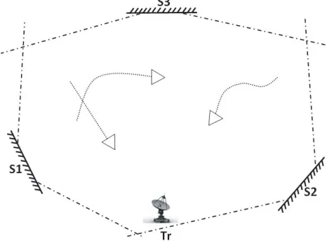
Consider the scenario illustrated in Figure 1, where an environment E contains a set of T targets. Neither the number of targets nor the states of each target are known at any given time step k, and they must be estimated. A set of sensing systems S are used to monitor E.
Each sensor outputs a set of detected DOAs at time t. A target with state xit in ith iteration is detected with probability Pd(xit). If it is detected, the measurement is characterized by the likelihood g(zt|i xit).
Figure 1. Three sensing system nodes S1, S2 and S3 detect common targets. Each node measures the DOA and transfers them to fusion center.
Figure 2. The relative situation of transmitter, receiver and target.
optimal way to achieve this is passing all sensing systems observations to a central site where they would be fused together [18].
2.1. RCS and SNR Prediction
There are various computational methods to predict RCS such as Physical Optics approximation (PO) [19], Physical Theory of Diffraction (PTD) [20], Uniform Geometrical Theory of Diffraction (UGTD) [21], and full-wave methods [22]. Since the physical dimensions of the mentioned structure are small with respect to the wavelength, instead of high frequency methods, full-wave methods can be used to analyze the structure. Method of Moments (MoM) [23] is the most suitable one for predicting RCS of conductive bodies. In other words, only the surface of the structure is meshed, so the number of unknowns is low with respect to other full-wave methods, like Finite Element Methods (FEM) and Finite Difference Time Domain methods (FDTD).
It is supposed that the target is moving with angle θh (with respect to the horizon) as shown in
Figure 2. T and R stand for the location of the transmitter and receivers, respectively. The transmitted wave reaches the target with angle θtr and returns to the receivers with angle θre. With the aid of
some simple geometrical relations, the angle of the incident wave with respect to the target noseθin is
calculated as:
θin= 180−(θh−θtr) (1) θout, the angle of the reflected wave to the receiver with respect to the nose of the target is given by:
θout= 180−(θh−θre) (2)
The bistatic RCS of the target has been evaluated from an oblique impinging plane wave. The oblique incident angle θin ranging from 0 to 360 degrees is shown in Figure 2. For each value of θin,
RCS has been recorded for all values of θout that varies from 0 to 360 degrees. Given θin and θout the
RCS of target is known.
Based on the bistatic radar equation, the received power in the receiver is:
Pr =
PtGtGrλ2σ
(4π)3R2
ttR2trL
(3)
where Rtt and Rtr are targets’ distances to transmitter and receivers; Pt and Pr are transmitted and
received powers; Gt and Gr are transmitter and receiver gains, respectively. λ,σ, and L are the signal
wavelength, RCS and atmospheric loss, respectively. Thus, SNR in receivers is: SNR = Pr
KT BF =C∗
σ(θin, θout) R2
ttR2trL
wherek, T, B and F are Boltzmann’s constant (1.38∗10−23J/◦K), absolute temperature of the receiver input (290◦K), receiver bandwidth, and noise figure/factor, respectively. The constant value C and σ
are defined as:
C = PtGtGrλ 2
(4π)3KT BF (5)
σ(θin, θout) =
360
i=1
N g
j=1
ωijN(θout;mij, Pij)δ(θin−i) (6)
in which δ denotes the kronecker delta, and N(x;m, P) denotes a Gaussian density with mean m and covariance matrixP. N gis the number of fitted Gaussians to the computed RCS. Signal with this SNR enters the receivers in order to estimate DOAs.
2.2. Detection
Observations are the result of detection operation. In this work, the transmitter scans the environment and in case of hitting the transmitter wave by the target, each receiver receives a signal with a different SNR, where the received SNR depends on the target’s RCS, based on the radar equation.
As stated in [24], RCS is a function of frequency, target shape, angles between the target to transmitter and receivers, etc. Thus, the target’s RCS varies from different receivers’ point of view. SNR of the received signal specifies the quality of DOA estimation. The suggested DOA estimation algorithm used in the proposed method is the Toeplitz-based method presented in [16], and its performance is compared with MUSIC and MUSIC-like. As mentioned before, MUSIC algorithm needs to know the number of targets, so it is more accurate than the two others. After DOA estimation, according to intersection of the transmitter beam direction and DOAs, the targets positions are evaluated in a Cartesian coordinate. Then the measurements are changed from DOA angles to [x, y] data. In addition, measurements to states relation are changed to linear. These data are sent to fusion center for multi-target multi-sensor filtering.
2.3. Tracking
The duty of Mahler’s RFS multi-target filtering [6] is the estimation of the number of targets and their states, rejection of clutter and accounting for missed detections. The RFS formulation for multi-target Bayesian filtering is the extension of the well-known single-target Bayesian filtering with sequentially computing the prediction and update steps as follows:
ft|t−1(Xt|Z1:t−1) =
ft|t−1(Xt|Xt−1)ft−1|t−1(Xt−1|Z1:t−1)δXt−1 (7)
ft|t(Xt|Z1:t) =
ft|t(Zt|Xt)ft|t−1(Xt|Z1:t−1)
ft|t
Zt|Xt
ft|t−1
Xt| Z1:t−1
δXt
(8)
where ft|t−1 is the multi-target predictive density, ft|t the multi-target posterior density, and Z1:t the
concatenation of all previous measurements up to time t.
Under certain assumptions and using finite set statistics (FISST) [6, 9], the PHD intensities can be recursively estimated as follows:
Dt|t−1(xt|Z1:t−1) = bt(xt) +
Ft|t−1(xt|xt−1)Dt−1|t−1(xt−1|Z1:t−1)dxt−1 (9)
Dt|t(xt|Z1:t) = [1−pD(xt)]Dt|t−1(xt|Z1:t−1)
zt∈Zt
ψzt(xt)Dt|t−1(xt|Z1:t−1)
κt(zt) +
ψzt(ξ)Dt|t−1(ξ|Z1:t−1)dξ (10)
At the prediction step in Equation (9):
whereft|t(xt|xt−1) is the single target transition pdf, and pS is the probability of target survival.
At the update step in Equation (10)
ψzt(xt) =pD(xt)g(zt|xt) (12)
wherepD is the probability of detection,g(zt|xt) the single target detection likelihood model, andκt(zt)
the intensity of the clutter points [6].
Nevertheless, a Gaussian mixture (GM) implementation can provide a closed form solution to the PHD filter for the special case where the target dynamics follow a linear Gaussian model [25]. Due to its closed form solution, GM-PHD is more accurate. In addition, it does not suffer from the sampling and resampling complexities encountered in particle based methods. In this paper, since it is reasonable to assume that our measurements and target state dynamics follow a linear/Gaussian model, GM-PHD is used for the multi-source filtering.
2.4. GMPHD Filter
Linear Gaussian multi-target models bring the PHD recursion to a closed form solution [25]. If (1) Linear Gaussian dynamical model and linear Gaussian measurement model for single target:
f(x|xt) = N(x;Ftxt, Qt) (13) gk(z|xt) = N(z;HtxtRt) (14)
where Ft, Qt, Ht and Rt are the state transition, process noise covariance, observation and observation
noise covariance matrices, respectively.
(2) State independent survival and detection probabilities:
PS,t+1|t(xt) = Ps,t+1 (15)
PD,t(xt) = PD,t (16)
(3) Gaussian mixtures for the intensities of the newly born targets RFS:
γt(x) = jγ,t
i=1
ω(γ,ti)N
x;m(γ,ti)Pγ,t(i)
(17)
(4) Gaussian mixtures for the prior intensity:
υ0(x) =
J0
i=1
ω0(i)N(x;m0(i), P0(i)) (18)
Then all subsequent predicted intensities υt+1|t and posterior intensities υk are also Gaussian
mixtures, i.e., GMPHD closed form solution follows the form of Gaussian mixtures for both prediction and update formulations.
υt+1|t(x) =υS,t+1|t(x) +γt+1(x) (19) in which
υs,t+1|t(x) = pS,t+1
Jk
j=1
ω(tj)N
x;Ftm(tj), Qt+FtPt(j)FtT
(20)
υt+1|t+1(x) = (1−pD,t+1)υt+1|t(x) +
z∈Zt+1
υD,t+1(x;z) (21)
in which
υD,t+1(x;z) =
Jt+1|t
j=1
ωt(+1j) (z)N
x;m(t+1j)|t+1, Pt(+1j)|t+1
(22)
ωt(+1j) (z) = pD,t+1ω (j)
t+1|tq
(j)
t+1(z)
ct+1(z) +pD,t+1
Jt+1|t
l=1
ωt(+1l) |tq(t+1l) (z)
qt(+1j) (z) = N
z;Ht+1m(tj+1)|tRt+1+Ht+1Pt(+1j)|tHtT+1
(24)
mt(+1j)|t+1(z) = mt(j+1)|k+Kt(j)
z−Ht+1m(t+1j)|t
(25)
Pt(+1j)|t+1 =
I −Kt(+1j)Ht+1
Pt(+1j)|t (26)
Kt(+1j) = Pt(+1j)|tHtT+1
Ht+1Pt(+1j)|tHtT+1+Rt+1
−1
(27) Since the Gaussian mixture representation of the posterior intensity υt is computed, multi-target
state estimation can be applied using the means of constituent Gaussian components with weight larger than a predefined threshold. Furthermore, GMPHD can easily be extended to nonlinear target dynamics models [26].
One of the most important drawbacks in custom multi-target multi-sensor tracking simulations is that targets data in each sensor are generated independently, while the targets are dependent in the case of cross or parallel. In the case of separate targets it is true, but when targets cross or parallel with each other, due to transmitter and receiver resolution, number of measurements in the neighbor of cross area is less than the number of targets. In other words, two targets are detectable only if their distance is more than the receivers range and azimuth resolution.
Knowledge of detection profile parameter is of critical importance in Bayesian multi-target filtering. Significant mismatches in clutter rate and detection profile model parameters inevitably result in erroneous estimates [27].
Another significant issue is that the data in each sensor are independently generated with deterministic and known probability of detection, and then the comparison is investigated for different Pds. It is concluded in [12, 28] that the more the Pd (the more data are achieved) is, the less the filtering failure is, and vice versa. It is obvious that in practice, Pd is unknown and should be estimated and assigned for each sensor. While working with real sensors, considering Pd of each sensor as a known parameter is a weaknes. Some articles have worked on estimating Pd of sensors [25, 29]. However, since the probability of detection in tracking stealth and low-observable targets is low, and the detection profile may change rapidly compared to the measurement update rate, their method cannot be utilized in the present work.
The assumption of Pd in the stealth target issue would have a great impact on the filtering results. A simple and routine way for modeling Pd is approximating it with some Gaussians as a function of states and using it in Equation (23) as in [25]. However, regarding nonlinear relationship between heading and states and also the effect of θtr,θre in evaluating θin,θout Pd cannot be approximated.
In the present work, parameters Pd and number of targets are supposed to be unknown, and transmitter and receiver resolution effects are also taken into account. The Pd belongs to the DOA estimation step and is a function of input SNR. This is compared for three different methods of DOA estimation for different SNRs and different numbers of targets.
3. NUMERICAL STUDY
3.1. RCS Estimation
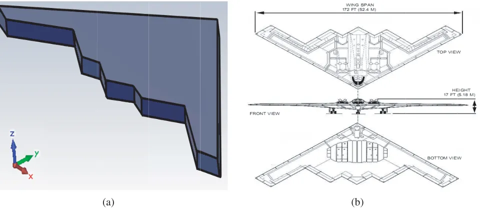
In this paper, the “integral equation solver” of commercial software CST Microwave Studio [30] is used. The exact schematic and dimensions of a simplified model of the B2 bomber aircraft are shown in Figures 3(a) and (b), respectively. A scheme with real size is exploited as a stealth aircraft. The model RCS is obtained for a collection of incident and reflected angles. The incident plane wave has a horizontal polarization, and its direction is specified with (θ, ϕ) in conventional spherical coordinates. The angle ϕ rotates from 0 to 360 degrees in steps of one. To obtain a real oblique simulation for the incident wave considering the transmitter and aircraft relative heights, the angle θis kept at 93◦.
The simulation is carried out in VHF band at center frequency of 150 MHz, and a mesh cell size of 10 cm is adopted. 25300 mesh cells are used for target surface meshing. The dimensions of model are considered as the original ones.
(a) (b)
Figure 3. B2 bomber stealth aircraft, (a) model, (b) schematic and dimensions.
is used in Equation (4) for evaluating the SNR.
3.2. SNR Calculation and Pd Modeling
A signal with an SNR enters the DOA estimator receivers, and according to intersection of the transmitter beam direction and DOAs, the targets positions are evaluated in the Cartesian coordinate. In these problems, usually, Pd is a function of SNR, number of targets and DOA estimation algorithm. In the present work, DOA estimation for different SNRs, number of targets and algorithms is performed and shown in Figure 4. The SNR is varied from −25 dB to 15 dB, and the field of view for each sensor is considered from −80◦ to 80◦ equal to 160◦. The probability of detection is estimated using Monte-Carlo with 1000 different runs, where the real DOAs are chosen randomly. Estimated DOAs with at most 0.5 degree difference with real ones are approved as detections, and other DOAs
P d P d -25-20-15-10 0.2 0.4 0.6 0.8 1 d 1 1 2 3 -25-20-15-10 0.2 0.4 0.6 0.8 1 3 T d
0-5 0 5 10 15
SNR Target
0-5 0 5 10 15
Targets
SNR
5 -25-20-0 0.2 0.4 0.6 0.8 1 P d
5 -25-20-0 0.2 0.4 0.6 0.8 1 P d
15-10 -5 0 5
2 Targets
SNR
15-10 -5 0 5
4 Targets
SNR
10 15
10 15
Figure 4. Pd estimation vs. SNR using different algorithms: Toeplitz-based (blue line), Music-Like (green line) and Music (red line).
-25-20-15-10 2 4 6 N fa 1 -25-20-15-10 2 4 6 3 N fa
10 -5 0 5 10
SNR 1 Target
1 2 3
10 -5 0 5 10
Targets SNR 0 15 1 2 3 -25-200 2 4 6 N fa
0 15 -25-200 2 4 6
N fa
0-15-10 -5 0 5
2 Targets
SNR
0-15-10 -5 0 5
4 Targets
SNR
5 10 15
5 10 15
are considered to be false alarms that are represented in Figure 5.
It is obvious that increasing SNR leads to increase of Pd and decrease of false alarms. An increase in the number of targets leads to a lower Pd in high SNRs and more false alarms in low SNRs. Although Toeplitz-based DOA estimation method has no information about the number of targets, its Pd estimation results are very close to MUSIC algorithm.
Since Pd versus SNR results have pseudo linear behaviors, polynomial data fitting is used, and they are approximated via a fifth order polynomial. After evaluation of the received signal SNR, Pd is computed considering target location, incident angle and received signal angle. So this Pd model can be used while filtering and weight updating in Equation (23).
3.3. Multi-Sensor Filtering
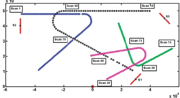
The performance of the proposed fusion algorithm is tested using the following tracking scenario: The targets initially move linearly, then maneuver with a coordinate turn model and finally return to linear dynamics. The trajectories cross points and iterations are shown in Figure 6. Moreover, three fixed sensors (S1, S2 and S3) with different orientations observe the environment E in which 4 targets appear, maneuver, cross, parallel and disappear over time. The state of each target is defined by its position [x, y] and velocity [ ˙x,y˙].
Figure 6. Trajectories and cross points of four targets in the scenario. Transmitter is located in (0, 0) and shown with red point. Receivers S1, S2 and S3 are shown with red lines.
The targets start moving in the 1st, 10th, 15th and 20th scans, respectively. In the 40th till 50th scans, targets parallel and then cross two by two. Then in the 70th scan, a cross happens for each target, and finally in the 90th scan, targets 2, 4 cross each other.
The tracks are obtained by evolving target states in accordance with a linear constant velocity motion model. The observation models are identical for all sensors, and the standard deviation in bearing is considered 2◦. The Pd of each sensor is independent of all other sensors.
In order to show the measurement error before filtering, OSPA metric was calculated between the real positions and estimated Cartesian ones. The outputs of different sensors and also tracking performances of different filters are compared using the optimal sub-pattern assignment (OSPA) error metric [31]. The OSPA error metric accounts for error in estimation of target states and number of targets. Given the two sets of estimated and true multi-target states, OSPA finds the best permutation of the larger set which minimizes its distance from the smaller set. We use the Euclidean distance metric and consider only the target positions while computing the OSPA error.
The Cartesian data are sent to fusion center for filtering. The OSPA metric for each sensor is illustrated in Figure 7. It is seen that OSPA varies with different scans due to different RCSs and ranges.
Figure 7. Measurement error in different receivers: Receiver#1 (green line), Receiver#2 (green line) and Receiver#3 (red line).
Figure 8. Single sensor and multi sensor filtering vs. assigned Pd. Sensor 1, 2 and 3, blue, green and orange, respectively, multi-sensor IC-PHD filter, pink and the proposed filter, black.
besides, up to 10 scans after it, each sensor has only one detection measurement instead of two. The worst thing is that the detected measurement is the average of targets positions. This leads to missing at least one target and may have a new target with erroneous states equal to average of two real targets. Since the simulations are based on reality, in addition to the RCS pattern, this important issue is taken into account.
In the following, in order to compare the performance of the proposed filter, the simulation results are compared once with single-sensor PHD filtering in each individual sensor and conventional IC-PHD filter. Then the proposed method performance is compared with IC-PHD, ICCPHD, G-PHD, G-CPHD filters.
The simulated observations are used by different filters to perform multi-target tracking. All the simulations were conducted using MATLAB. Pd is unknown in the proposed method, is considered variable, and is gradually increased from 0.1 to 0.9 in other algorithms. The tracking performances of different filters are compared using OSPA error metric. For the OSPA metric, the cardinality penalty factor C and power P are set to 10000 and 1, respectively.
We report the average OSPA error obtained by running each multi-sensor filter over these 100 observation sequences.
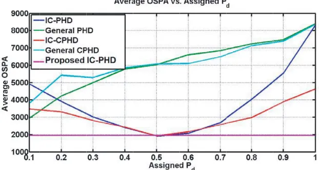
Figure 9 shows the average OSPA error as the probability of detection is changed. General PHD and CPHD filters which have a different mathematical base have the worst performances. Conventional IC-CPHD does better filtering than IC-PHD one. The proposed IC-PHD filter enhanced with Pd modeling performs significantly better than all other filters.
Figure 9. Average OSPA vs. assigned Pd for different multi sensor filtering.
4. CONCLUSION
In the present work, multi-target tracking of stealth targets is investigated for multi-static radar with passive receivers. The receivers estimate Direction of Arrival (DOA) of targets without knowing their numbers, and the targets positions are measured according to the transmitter beam direction. The first feature of this work is using the well-known commercial software CST-MWS for modeling the RCS of simplified B2 bomber aircraft model as a stealth target for a variety of incident and observation angles. To realize a practical situation, an oblique incident has been considered, and the results are fitted by a mixture of Gaussians. Using Toeplitz-based DOA estimation method and RCS pattern, Pd for each measurement is modeled and then fed to the IC-PHD filter. Thus, there is no need to know the number of targets and Pd of each sensor, which is the main feature of this work. The third feature is that the resolutions of the transmitter and receivers are also taken into account in our simulations. The simulation results show that the proposed method outperforms the previous conventional filtering results.
REFERENCES
1. Pulford, G., “Taxonomy of multiple target tracking methods,” IEE Proceedings — Radar, Sonar and Navigation, Vol. 152, No. 5, 291, 2005.
2. Khaleghi, B., A. Khamis, F. Karray, and S. Razavi, “Multisensor data fusion: A review of the state-of-the-art,” Information Fusion, Vol. 14, No. 1, 28–44, 2013.
3. Vo, B.-N., M. Mallick, Y. Bar-Shalom, S. Coraluppi, R. Osborne III, R. Mahler, and B.-T. Vo, “Multitarget tracking,” Wiley Encyclopedia of Electrical and Electronics Engineering, Wiley, Sep. 2015.
4. Bar-Shalom, Y., X. Tian, and P. Willett,Tracking and Data Fusion, YBS Publishing, Storrs, Conn., 2011.
5. Blackman, S. and R. Popoli, Design and Analysis of Modern Tracking Systems, Artech House, Boston, 1999.
7. Mahler, R., Advances in Statistical Multisource-multitarget Information Fusion, Artech House, Boston, 2014.
8. Uney, M., D. Clark, and S. Julier, “Distributed fusion of PHD filters via exponential mixture densities,”IEEE Journal of Selected Topics in Signal Processing, Vol. 7, No. 3, 521–531, 2013. 9. Mahler, R., “Multi-target Bayes filtering via first-order multi-target moments,” IEEE Trans.
Aerosp. Electron. Syst., Vol. 39, No. 4, 1152–1178, Oct. 2003.
10. Mahler, R., “PHD filters of higher order in target number,”IEEE Trans. Aerosp. Electron. Syst., Vol. 43, No. 4, 1523–1543, 2007.
11. Nannuru, S., M. Coates, M. Rabbat, and S. Blouin, “General solution and approximate implementation of the multisensor multitarget CPHD filter,”Proc. IEEE ICASSP-15, 4055–4059, Brisbane, Australia, Apr. 2015.
12. Nannuru, S., S. Blouin, M. Coates, and M. Rabbat, “Multisensor CPHD filter,” IEEE Trans. Aerosp. Electron. Syst., Vol. 52, No. 4, 1834–1854, 2016.
13. Vivone, G., P. Braca, K. Granstrom, and P. Willett, “Multistatic Bayesian extended target tracking,”IEEE Trans. Aerosp. Electron. Syst., Vol. 52, No. 6, 2626–2643, 2016.
14. Barbary, M. and P. Zong, “An accurate 3-D netted radar model for stealth target detection based on Legendre orthogonal polynomials and TDOA technique,”International Journal of Modeling and Optimization, Vol. 5, No. 1, 22–31, Feb. 2015.
15. Schmidt, R. O., “Multiple emitter location and signal parameter estimation,” IEEE Transitions on Antennas and Propagation, Vol. 34, No. 3, 276–280, Mar. 1986.
16. Zhang, Y. and B. P. Ng, “MUSIC-like DOA estimation without estimating the number of sources,” IEEE Transactions on Signal Processing, Vol. 58, No. 3, 1668–1676, 2010.
17. Qian, C., L. Huang, W. Zeng, and H. So, “Direction-of-arrival estimation for coherent signals without knowledge of source number,”IEEE Sensors Journal, Vol. 14, No. 9, 3267–3273, 2014. 18. Li, W., Z. Wang, G. Wei, L. Ma, J. Hu, and D. Ding, “A survey on multisensor fusion and consensus
filtering for sensor networks,” Discrete Dynamics in Nature and Society, Vol. 2015, 1–12, 2015. 19. Harrington, R.,Time-harmonic Electromagnetic Fields, IEEE Press, New York, 2001.
20. Ufimtsev, P.,Method of Edge Waves in the Physical Theory of Diffraction, NTIS, Springfield, Va., 1980.
21. Kouyoumjian, R. and P. Pathak, “A uniform geometrical theory of diffraction for an edge in a perfectly conducting surface,”Proceedings of the IEEE, Vol. 62, No. 11, 1448–1461, 1974.
22. Yu, D. and M. Zhang, “Comparison of various full-wave methods in calculating the RCS of inlet,” 2008 International Conference on Microwave and Millimeter Wave Technology, 1018–1021, Nanjing, 2008.
23. Gibson, W. C.,The Method of Moments in Electromagnetics, CRC Press, 2014. 24. Skolnik, M., Radar Handbook, McGraw-Hill, New York, 2009.
25. Vo, B. and W. Ma, “The Gaussian mixture probability hypothesis density filter,” IEEE Transactions on Signal Processing, Vol. 54, No. 11, 4091–4104, 2006.
26. Huang, Z., S. Sun, and J. Wu, “A new data association algorithm using probability hypothesis density filter,”Journal of Electronics (China), Vol. 27, No. 2, 218–223, 2010.
27. Mahler, R., B. Vo, and B. Vo, “CPHD filtering with unknown clutter rate and detection profile,” IEEE Transactions on Signal Processing, Vol. 59, No. 8, 3497–3513, 2011.
28. Saucan, A.-A., M. Coates, and M. Rabbat, “A multi-sensor multi-Bernoulli filter,” IEEE Transactions on Signal Processing, Vol. 65, No. 20, 5495–5509, 2017.
29. Vo, B., B. Vo, R. Hoseinnezhad, and R. Mahler, “Robust multi-bernoulli filtering,” IEEE Journal of Selected Topics in Signal Processing, Vol. 7, No. 3, 399–409, 2013.
30. CST Microwave Studio, Computer Simulation Technology AG [Online], available: http://www.cst-america.com.