Non-Reciprocal Antenna Array Based on Magnetized Graphene
for THz Applications Using the Iterative Method
Aymen Hlali*, Zied Houaneb, and Hassen Zairi
Abstract—An effective and precise approach to the Wave Concept Iterative Process method modeling of magnetized graphene sheet as an anisotropic conductive surface is used to analyze the anisotropy of magnetostatically biased graphene and for studying an electrically doped magnetically biased graphene non-reciprocal antenna array for THz applications. The tuning of the performance of the array antenna is possible by varying the magnetic field and the chemical potential of graphene material. The return loss value decreases by increasing the magnetostatic bias and increases when the chemical potential increases.
1. INTRODUCTION
Non-reciprocal components are ubiquitous in electronic and optical systems. According to recent progress in graphene research, it has been shown that graphene exhibits gyrotropic properties, making it a promising candidate for the realization of non-reciprocal devices [1–4]. Furthermore, the combined application of magnetic bias and electrical doping in graphene can be leveraged towards tunable and versatile non-reciprocal plasmonic components. Several groups have proposed non-reciprocal components based on graphene’s such as antennas, couplers, circulators, phase shifters, and other non-reciprocal devices [5–10].
Along with this research process, new methods are much in demand to model-based electronic devices based on the magnetized graphene [10–15]. In most of the numerical methods, magnetized graphene is usually incorporated in the algorithm by transforming the surface conductivity to a volumetric conductivity by dividing the thickness of the graphene, which might introduce a multiscale computational problem in simulation, require massive CPU time and memory, and make the optimization process tiresome. In order to overcome this problem, the wave concept iterative process method can be applied by treating the 2D materials as conductive surface boundaries, to not only yield precision in the result, but also reduce the time consumption and memory size [16–25].
In summary, we investigate a reconfigurable and non-reciprocal antenna array based on magnetized graphene over an ultrawide terahertz band using the Wave Concept Iterative Process method. In particular, the response of the proposed array antenna can be controlled conveniently by adjusting the chemical potential and the magnetic field of graphene. The remaining part of this paper is organized as follows. In Section 2, some theoretical aspects about the anisotropic surface conductivity of graphene and a brief overview to the WCIP method are described. Section 3 investigates numerical results to demonstrate the capability of the proposed algorithm for the modeling and simulation of non-reciprocal antenna array for THz applications. Some conclusions are presented in Section 4.
Received 22 November 2019, Accepted 16 January 2020, Scheduled 30 January 2020
* Corresponding author: Aymen Hlali ([email protected]).
2. THEORY AND FORMULATION
2.1. Conductivity Model of Magnetized Graphene
The magnetized graphene is an infinitesimally thin sheet biased by a magnetostatic field and behaves as an anisotropic conducting sheet characterized by a conductivity tensor [26–29]
¯ ¯ σ=
σd −σo
σo σd
(1)
The expressions of σd and σo can be approximated by a Drude-like model [14, 28], which are
σd = σ
1 +jωτ (ωcτ)2+ (1 +jωτ)2
(2)
σo = σ( ωcτ
ωcτ)2+ (1 +jωτ)2
(3)
with
σ = e 2τ K
BT
π2
μc
KBT
+ 2 ln
e−KBTµc + 1
(4)
where τ is the phenomenological scattering time, ωc = eBv
2
F
μc the cyclotron frequency, B the amplitude
of the static magnetic field bias, e the electron charge, KB the Boltzmann constant, T the room
temperature, vF the Fermi velocity,μc the chemical potential, andthe reduced Plancks constant.
2.2. Formulation of WCIP Method
The classic WCIP method has been described in detail in various articles [16–25]. This method is presented by writing the electric field and current density in terms of waves. We can express these combinations by the following equations
Ai =
1 2√Z0i
(Ei+Z0iJi) i= 1,2 (5)
Bi =
1 2√Z0i
(Ei−Z0iJi) i= 1,2 (6)
where Ai and Bi are, respectively, the incident and the reflected waves. Z0i is the characteristic
impedance of the middle i (i = 1,2) given by Z0i =
μ0
ε0εri where εri is the relative permittivity
of the region i. Ji is the surface tangential current density which defineJi =Hi×ni.
2.3. Formulation of the Magnetized Graphene in WCIP Method
The implementation of the boundary conditions of the magnetized graphene in the WCIP method has been demonstrated in detail in this article [25]. After some manipulation, we can derive the scattering matrix of the magnetized graphene as
⎛ ⎜ ⎜ ⎝ B1,x B1,y B2,x B2,y ⎞ ⎟ ⎟ ⎠= ⎛ ⎜ ⎜ ⎜ ⎝
S11Gm SGm12 S13Gm S14Gm SGm
21 SGm22 S23Gm S24Gm SGm
31 SGm32 S33Gm S34Gm S41Gm SGm42 S43Gm S44Gm
⎞ ⎟ ⎟ ⎟ ⎠ ΓGm ⎛ ⎜ ⎜ ⎝ A1,x A1,y A2,x A2,y ⎞ ⎟ ⎟ ⎠
whereSijGm are defined by
S11Gm =
X4X1−X22 X2
1 +X22
; S12Gm=
X4X2 X2
S13Gm =
2X1(Z02√Z01) X2
1 +X22
; SGm14 = 2σo
√
Z01(Z02√Z01)2 X2
1 +X22
S21Gm =
−2σo(Z02 √
Z01)2 X12+X22
; S22Gm=S11Gm; S31Gm=
2X1(Z01√Z02)
√
Z01[X12+X32]
S23Gm =
−2σo(Z02 √
Z01)2
√
Z02[X12+X22]
; S24Gm=
2X1(Z02√Z01)
√
Z02[X12+X22]
S32Gm =
2σo(Z01 √
Z02)2 X2
1 +X32
; S33Gm =
X5X1−X32 X2
1 +X32
; S34Gm =S32Gm
S41Gm =
−2σo √
Z02(Z01
√
Z02)2
√
Z01(X12−X32)
; S42Gm =
2X1(Z01√Z02)
√
Z01(X12−X32)
S43Gm =
−2σo(Z01 √
Z02)2 X12−X32
; S44Gm=
X5X1−X2 3 X12−X32 and
X1 = Z02+Z01+σdZ01Z02 (7)
X2 = (σo √
Z01)(Z02
√
Z01) (8)
X3 = (σo √
Z02)(Z01
√
Z02) (9)
X4 = Z02−Z01−σdZ01Z02 (10)
X5 = Z01−Z02−σdZ01Z02 (11)
3. NUMERICAL RESULTS AND DISCUSSION
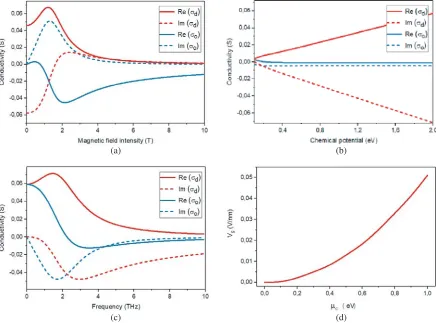
According to the conductivity, there are different scenarios for the properties of the material. The usual case is obtained when the properties are not dependent on the direction; this is the case of the isotropic graphene. Contrary to the case of isotropic surfaces, the anisotropic case occurs when the parts of the conductivity components are different Im(σd) = Im(σo) and Re(σd) = Re(σo). Fig. 1 illustrates the surface conductivityσd and σo of a graphene sheet. The variation of the graphene conductivity versus
the biasing magnetostatic fieldsB and the chemical potential μc is simulated at 2 THz.
Obtained results prove a high anisotropy of the conductivity components. It is clear from these figures that two parameters can control conductivity: the magnetic fieldB and the chemical potential μc. Note that in conventional gyrotropic material, such as ferrites, the constitutive parameters depend
only on the magnetic field. In graphene, the chemical potentialμc can be controlled via an electrostatic
potential. Fig. 1(d) presents the relationship between bias voltage and chemical potential for an Arlon substrate with thickness 3µm.
Next, in order to demonstrate the accuracy of the proposed algorithm for modeling of non-reciprocal devices, a program in FORTRAN has been written to simulate a non-reciprocal antenna array for THz applications. The array antenna is placed in the xy-plane and biased by a magnetic field, B, in the z-axis direction. As shown in Fig. 2, an antenna array is printed on an Arlon substrate with dielectric constant ofr = 3 which is typically illuminated by an x-polarized plane wave. The length and width
of the substrate are kept fixed at 100µm and 60µm, respectively, whereas the height is 3µm. The gray area represents the graphene, and the white area describes the dielectric substrate.
In order to examine the results obtained by the WCIP method, we begin by studying the boundary conditions. Fig. 3 shows the variation of the reflection coefficient as a function of the number of iterations at the resonant frequency. We find that the convergence is obtained from 300 iterations.
Figures 4(a) and 4(b) illustrate the current density distribution|Jx|and the electric field distribution
|Ex|of the proposed structure. According to these figures, we notice that the electric field and current
(a) (b)
(c) (d)
Figure 1. Variation of graphene conductivity versus: (a) Biasing magnetostatic fields B, (b) chemical potentialμc, (c) frequency, and (d) relationship between bias voltage and chemical potential. Graphene
parameters are selected asτ = 0.1 ps,T = 300 K.
(a) (b)
Figure 2. Schematic of the proposed array antenna: (a) Top view, and (b) geometric parameters of the radiation patch. Parameters are W1 = 12.8µm, W2 = 4.26µm, W3 = 10.24µm, W4 = 21.33µm, L1 = 28.16µm, L2 = 8.96µm,L3= 87.04µm, a= 10.24µm, b= 2.56µm, c= 28.16µm, d= 45◦.
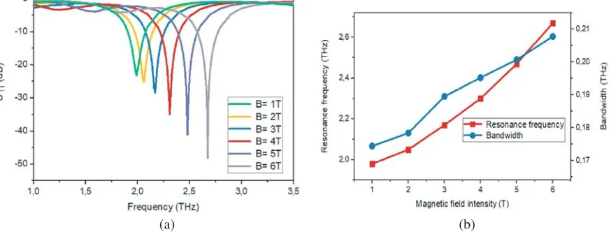
Further, we study the influences of graphene parameters on the antenna array performances. Fig. 5 shows the simulation results obtained under the chemical potential of 0.5 eV with different magnetostatic bias.
Figure 5(b) shows the tunability of the resonance frequency fr and the bandwidth Δfr with
Figure 3. Convergence of the reflection coefficient S11 versus number of iterations.
(a) (b)
Figure 4. (a) Distribution of the current density of the interface |Jx|, and (b) distribution of the
electric field of the interface |Ex|.
(a) (b)
Figure 5. (a) Simulated results for different magnetic fields, and (b) variation of resonance frequency and bandwidth.
increased from 1.98 to 2.67 THz, and Δfr is varied from 0.173 to 0.203 THz. It can be seen that the
return loss value decreases by increasing the magnetostatic bias.
the magnetostatic bias is 1 T are shown in Fig. 6. It can be seen from Fig. 6(b) that the maximum value increases when the chemical potential increases, and the resonant frequency shifts toward high frequencies with higher amplitude.
The E and H-planes radiation patterns properties of the antenna array are shown in Fig. 7. The results show that the parameters of graphene have significant impacts on the magnitude of the lobe in the E-plane and H-plane, in which the radiation pattern becomes more directive by increasing the magnetic field and chemical potential.
(a) (b)
Figure 6. (a) Simulated results for different chemical potentials, and (b) variation of resonance frequency and bandwidth.
(a) (b)
Figure 7. (a) Radiation pattern in theE-plane, and (b) radiation pattern in theH-plane.
4. CONCLUSION
REFERENCES
1. Crassee, I., J. Levallois, A. L. Walter, M. Ostler, A. Bostwick, E. Rotenberg, T. Seyller, D. D. Marel, A. B. Kuzmenko, “Giant Faraday rotation in single-and multilayer graphene,” Nature Physics, Vol. 7, 48–51, 2011.
2. Sounas, D. L. and C. Caloz, “Electromagnetic nonreciprocity and gyrotropy of graphene,”Applied Physics Letters, Vol. 98, 021911, 2011.
3. Sounas, D. L. and C. Caloz, “Edge surface modes in magnetically biased chemically doped graphene strips,”Applied Physics Letters, Vol. 99, 231902, 2011.
4. Sounas, D. L. and C. Caloz, “Gyrotropy and nonreciprocity of graphene for microwave applications,” IEEE Transactions on Microwave Theory and Techniques, Vol. 60, 901–914, 2012. 5. Serrano, D. C., J. S. G. Diaz, D. L. Sounas, Y. Hadad, A. A. Melcon, and A. Al`u, “Nonreciprocal
graphene devices and antennas based on spatiotemporal modulation,”IEEE Antennas and Wireless Propagation Letters, Vol. 15, 1529–1532, 2016.
6. Zhu, B., G. Ren, Y. Gao, B. Wu, Q. Wang, C. Wan, and S. Jian, “Graphene plasmons isolator based on non-reciprocal coupling,”Optics Express, Vol. 23, 16071–16083, 2015.
7. Tamagnone, M., C. Moldovan, J. M. Poumirol, A. B. Kuzmenko, A. M. Ionescu, J. R. Mosig, and J. P. Carrier, “Near optimal graphene terahertz non-reciprocal isolator,”Nature Communications, Vol. 7, 11216(1-6), 2016.
8. Serrano, D. C., J. S. G. Diaz, A. Al`u, and A. ´A. Melc´on, “Electrically and magnetically biased graphene-based cylindrical waveguides: analysis and applications as reconfigurable antennas,”
IEEE Transactions on Terahertz Science and Technology, Vol. 5, 951–960, 2015.
9. Chamanara, N., D. Sounas, and C. Caloz, “Non-reciprocal magnetoplasmon graphene coupler,”
Optics Express, Vol. 21, 11248–11256, 2013.
10. Tamagnone, M., A. Fallahi, J. R. Mosig, and J. P. Carrier, “Fundamental limits and near-optimal design of graphene modulators and non-reciprocal devices,” Nature Photonics, Vol. 8, 556–563, 2014.
11. Feizi, M., V. Nayyeri, and O. M. Ramahi, “Modeling magnetized graphene in the finite-difference time-domain method using an anisotropic surface boundary condition,” IEEE Transactions on Antennas and Propagation, Vol. 66, 233–241, 2018.
12. Amanatiadis, S. A., N. V. Kantartzis, T. Ohtani, and Y. Kanai, “Precise modeling of magnetically-biased graphene through a recursive convolutional FDTD method,” IEEE Transactions on Magnetics, Vol. 54, 233–241, 2018.
13. Wang, X. H., W. Y. Yin, and Z. Chen, “Matrix exponential FDTD modeling of magnetized graphene sheet,” IEEE Antennas and Wireless Propagation Letters, Vol. 12, 1129–1132, 2013. 14. Cao, Y. S., P. Li, L. J. Jiang, and A. E. Ruehli, “The derived equivalent circuit model for magnetized
anisotropic graphene,”IEEE Antennas and Wireless Propagation Letters, Vol. 65, 948–953, 2017. 15. Shao, Y., J. J. Yang, and M. Huang, “A review of computational electromagnetic methods for
graphene modeling,”International Journal of Antennas and Propagation, Vol. 81, 1–6, 2016. 16. Azizi, M., M. Boussouis, H. Aubert, and H. Baudrand, “A three-dimensional analysis of planar
discontinuities by an iterative method,”Microwave and Optical Technology Letters, Vol. 13, 372– 376, 1996.
17. N’gongo, R. S. and H. Baudrand, “A new approach for microstrip active antennas using modal FFT algorithm,”IEEE Antennas and Propagation Society International Symposium, Vol. 3, 1700–1703, 1999.
18. Gharsallah, A., A. Gharbi, and H. Baudrand, “Efficient analysis of multiport passive circuits using the iterative technique,” Electromagnetics, Vol. 81, 73–84, 2001.
20. Mami, A., H. Zairi, A. Gharsallah, and H. Baudrand, “Analysis of microwave components and circuits using the iterative method,”International Journal of RF and Microwave, Vol. 81, 404–414, 2004.
21. Aizi, M., H. Aubert, and H. Baudrand, “A new iterative method for scattering problems,”
Microwave Conference, Vol. 1, 255–258, 1995.
22. Houaneb, Z., H. Zairi A. Gharsallah, and H. Baudrand, “Modeling of cylindrical resonators by wave concept iterative process in cylindrical coordinates,”International Journal of Numerical Modelling: Electronic Networks, Devices and Fields, Vol. 24, 123–131, 2011.
23. Hlali, A., Z. Houaneb, and H. Zairi, “Tunable filter based on hybrid metal-graphene structures over an ultrawide terahertz band using an improved Wave Concept Iterative Process method,”
International Journal for Light and Electron Optics, Vol. 181, 423–431, 2018.
24. Hlali, A., Z. Houaneb, and H. Zairi, “Dual-band reconfigurable graphene-based patch antenna in terahertz band: Design, analysis and modeling using WCIP method,”Progress In Electromagnetics Research C, Vol. 87, 213–226, 2018.
25. Hlali, A., Z. Houaneb, and H. Zairi, “Effective modeling of magnetized graphene by the wave concept iterative process method using boundary conditions,” Progress In Electromagnetics Research C, Vol. 89, 121–132, 2019.
26. Hanson, G. W., “Dyadic Green’s functions for an anisotropic, non-local model of biased graphene,”
IEEE Transactions on Antennas and Propagation, Vol. 103, 101–109, 2008.
27. Lovat, G., “Equivalent circuit for electromagnetic interaction and transmission through graphene sheets,”IEEE Transactions on Electromagnetic, Vol. 54, 101–109, 2012.
28. Li, P. and L. J. Jiang, “Modeling of magnetized graphene from microwave to THz range by DGTD with a scalar RBC and an ADE,” IEEE Transactions on Antennas and Propagation, Vol. 63, 4458–4467, 2015.