Numerical Simulation of Fragment-Type Antenna by Using Finite
Difference Time Domain (FDTD)
Li-Xia Yang, Xiao-Dong Ding, Da-Wei Ding*, and Jing Xia
Abstract—Finite Difference Time Domain (FDTD) method is widely used in the simulation of various kinds of antennas. In this paper, research on the numerical simulation of the fragment-type antenna by using FDTD is conducted. The fragment-type antenna structures with different cell sizes and different overlapping sizes are simulated and measured. The validity of the numerical simulation of the fragment-type antenna by using FDTD is verified through the comparison between the simulated and measured return losses. In addition, its efficiency in terms of computation time shows great potential in engineering applications, especially when the design matrix is large enough.
1. INTRODUCTION
Fragment-type structure has found many successful applications in the antenna field [1–5]. In [1, 2], a fragment-type structure is utilized to design broadband and dual-band microstrip antennas. A circular polarization microstrip antenna is designed by employing a fragment-type structure in [3]. In [4], the concept of type structure is introduced to design a reconfigurable antenna. Compact fragment-type antenna is shown in [5].
Compared with the antennas with regular structures, a fragment-type antenna can be designed with higher filling efficiency and more design freedom in a given design region. Therefore, fragment-type structure is promising for compact antenna, antenna with novel structure, and antenna with higher electrical performance.
It is well known that a fragment-type antenna is mainly optimized by using evolutionary algorithms (EAs), such as Genetic Algorithm (GA) [6] and Multiobjective Evolutionary Algorithm Based on Decomposition combined with Enhanced Genetic Operators (MOEA/D-GO) [7]. In these EAs, fitness evaluation is necessary, which corresponds to simulation of the electrical parameters of a fragment-type antenna. There are some candidates for the stimulation of a fragment-fragment-type antenna, such as Computer Simulation Technology (CST) [8], High Frequency Structure Simulator (HFSS) [9], and FDTD Simulation software (XFDTD) [10]. However, those methods are extremely computationally expensive. Finite Difference Time Domain (FDTD) source code becomes an excellent solution because of its following features,
1) it is easy to obtain electrical characteristics over broadband through a single run in time domain, 2) those cells of the fragment-type structure can be consistent with the generated cells in the FDTD
implement, and
3) parallel version of FDTD has been widely used.
Received 11 November 2016, Accepted 17 March 2017, Scheduled 27 March 2017
* Corresponding author: Da-Wei Ding ([email protected]).
Although FDTD source code has been used for numerical simulation of fragment-type antennas [11, 12], there is no work on investigating the numerical simulation of fragment-type antennas with different cell sizes and different overlapping dimensions. Moreover, there is no research on validating its efficiency when the design matrix of the fragment-type structure is large enough.
This paper simulates a fragment-type antenna by using FDTD method, studies the influence of different cell sizes and overlapping sizes on the simulation results, and verifies the high efficiency of FDTD through the comparison among the simulation results.
The paper is organized as follows. The algorithm principle of FDTD is reviewed simply in Section 2. Fragment-type structure and its simulation by using FDTD are demonstrated in Section 3. In Section 4, we study the simulated and measured results of the fragment-type antenna structures with different cell sizes and overlapping sizes. In Section 5, a conclusion and prospect for the research work of this paper is presented.
2. FDTD PRINCIPLE
2.1. Governing Equations
FDTD method starts from the differential form of Maxwell’s two curl equations as shown in Eqs. (1) and (2). To keep it simple in this article, the media are assumed to be lossless and isotropic. On the basis of these assumptions, Maxwell’s curl equations may be written as
∇ ×E = −∂B
∂t −Jm (1)
∇ ×H = ∂D
∂t +J (2)
whereE,H,DandB represent electric field intensity, magnetic field intensity, electric flux density, and magnetic flux density, respectively. J andJmrepresent electric current density and equivalent magnetic
current density. The finite difference approximations to Eqs. (1) and (2) are
En+1
xi+1/2,j,k = ⎛ ⎜ ⎜ ⎜ ⎝
1−σi+1/2,j,kΔt 2εi+1/2,j,k
1 +σi+1/2,j,kΔt 2εi+1/2,j,k
⎞ ⎟ ⎟ ⎟
⎠·Exin+1/2,j,k+ ⎛ ⎜ ⎜ ⎜ ⎝ Δt εi+1/2,j,k
1 +σi+1/2,j,kΔt 2εi+1/2,j,k
⎞ ⎟ ⎟ ⎟ ⎠ · ⎛ ⎝H
n+1/2
zi+1/2,j+1/2,k−H n+1/2
zi+1/2,j−1/2,k
Δy −
Hn+1/2
yi+1/2,j,k+1/2−H
n+1/2
yi+1/2,j,k−1/2 Δz
⎞
⎠ (3)
En+1
yi,j+1/2,k = ⎛ ⎜ ⎜ ⎜ ⎝
1−σi,j+1/2,kΔt 2εi,j+1/2,k
1 +σi,j+1/2,kΔt 2εi,j+1/2,k
⎞ ⎟ ⎟ ⎟
⎠·Eyi,jn +1/2,k+ ⎛ ⎜ ⎜ ⎜ ⎝ Δt εi,j+1/2,k
1 + σi,j+1/2,kΔt 2εi,j+1/2,k
⎞ ⎟ ⎟ ⎟ ⎠ · ⎛ ⎝H
n+1/2
xi,j+1/2,k+1/2−H
n+1/2
xi,j+1/2,k−1/2
Δz −
Hn+1/2
zi+1/2,j+1/2,k−H n+1/2
zi−1/2,j+1/2,k
Δx
⎞
⎠ (4)
En+1
zi,j,k+1/2 =
⎛ ⎜ ⎜ ⎜ ⎝
1−σi,j,k+1/2Δt 2εi,j,k+1/2 1 +σi,j,k+1/2Δt
2εi,j,k+1/2
⎞ ⎟ ⎟ ⎟
⎠·Ezi,j,kn +1/2+
⎛ ⎜ ⎜ ⎜ ⎝ Δt εi,j,k+1/2
1 +σi,j,k+1/2Δt 2εi,j,k+1/2
⎞ ⎟ ⎟ ⎟ ⎠ · ⎛ ⎝H
n+1/2
yi+1/2,j,k+1/2−H
n+1/2
yi−1/2,j,k+1/2
Δx −
Hn+1/2
xi,j+1/2,k+1/2−H
n+1/2
xi,j−1/2,k+1/2 Δy
⎞
Hn+1/2
xi,j+1/2,k+1/2 =
⎛ ⎜ ⎜ ⎜ ⎝
1−σi,j+1/2,k+1/2Δt 2μi,j+1/2,k+1/2 1 + σi,j+1/2,k+1/2Δt
2μi,j+1/2,k+1/2
⎞ ⎟ ⎟ ⎟ ⎠·H
n−1/2
xi,j+1/2,k+1/2+
⎛ ⎜ ⎜ ⎜ ⎝ Δt μi,j+1/2,k+1/2
1 +σi,j+1/2,k+1/2Δt 2μi,j+1/2,k+1/2
⎞ ⎟ ⎟ ⎟ ⎠ · En
zi,j+1,k+1/2−Ezi,j,kn +1/2
Δy −
En
yi,j+1/2,k+1−Eyi,jn +1/2,k
Δz (6)
Hn+1/2
yi+1/2,j,k+1/2 =
⎛ ⎜ ⎜ ⎜ ⎝
1−σi+1/2,j,k+1/2Δt 2μi+1/2,j,k+1/2
1 + σi+1/2,j,k+1/2Δt 2μi+1/2,j,k+1/2
⎞ ⎟ ⎟ ⎟ ⎠·Hn−
1/2
yi+1/2,j,k+1/2+
⎛ ⎜ ⎜ ⎜ ⎝ Δt μi+1/2,j,k+1/2
1 +σi+1/2,j,k+1/2Δt 2μi+1/2,j,k+1/2
⎞ ⎟ ⎟ ⎟ ⎠ · En
xi+1/2,j,k+1−Exin+1/2,j,k
Δz −
En
zi+1,j,k+1/2−Ezi,j,kn +1/2
Δx (7)
Hn+1/2
zi+1/2,j+1/2,k = ⎛ ⎜ ⎜ ⎜ ⎝
1−σi+1/2,j+1/2,kΔt 2μi+1/2,j+1/2,k
1 + σi+1/2,j+1/2,kΔt 2μi+1/2,j+1/2,k
⎞ ⎟ ⎟ ⎟ ⎠·H
n−1/2
zi+1/2,j+1/2,k+ ⎛ ⎜ ⎜ ⎜ ⎝ Δt μi+1/2,j+1/2,k
1 +σi+1/2,j+1/2,kΔt 2μi+1/2,j+1/2,k
⎞ ⎟ ⎟ ⎟ ⎠ · En
yi+1,j+1/2,k−Eyi,jn +1/2,k
Δx −
En
xi+1/2,j+1,k−Exin+1/2,j,k
Δy (8)
where Δx, Δy and Δz represent the sizes along three directions of each unit cell, respectively, and Δt represents the time step. σ,εandμrepresent electric conductivity, electrical permittivity and magnetic permeability, respectively. i,j and kcorrespond to the node numbers of the unit cell in the ˆx, ˆy and ˆz directions.
2.2. Courant Stability Condition
Due to the numerical dispersion in the above approximations, the maximum time steps that may be used are limited
cΔt≤ 1 1
(Δx)2 + 1 (Δy)2 +
1 (Δz)2
(9)
2.3. Source Consideration
In this paper, a Gaussian pulse is considered as the excitation because it will provide frequency-domain information from dc to the desired cutoff frequency by adjusting the width of the pulse. For a more intuitive representation, the computational model is shown in Fig. 1. The vertical electric field is imposed in order to simulate a voltage source excitation. The time-domain form of Gaussian pulse can be expressed as
Ei(t) = 0.5∗exp
−(t−t0)
2
τ2 (10)
whereτ is constant, which determines the width of the Gaussian pulse. t0 is the moment of pulse peak. Because the antenna used in this paper works in 2 GHz–20 GHz, we set τ = 25 ps,t0 = 150 ps.
2.4. Input Resistance
Excitation y z
x
Figure 1. Computational model.
Fourier transform. The input impedance can be obtained as Zin= UIz
z
(11)
whereUz and Iz are the frequency responses of the transient voltage and current.
Then the reflection coefficient can be determined according to the formula S11(dB) = 20 lgZin−Zc
Zin+Zc
(12)
where Zc is the characteristic impedance, and it should be noted that the reference plane is different form the feed plane, which is chosen with enough distance from the circuit discontinuities to eliminate evanescent waves.
2.5. Absorbing Boundary
Due to the finite capabilities of the computer used to calculate the finite-difference equations, the mesh must be limited in the ˆx, ˆy and ˆz directions. Nearly Perfectly Matched Layer (NPML) proposed by Cummer [13] serves as absorption boundary in this paper because of its simplify for programming while maintaining the same absorbing ability as Perfectly Matched Layer. For the stability of calculation, we set the thickness of NPML as 6 grids to eliminate the reflection of electromagnetic waves appearing at the truncated mesh.
3. MICROSTRIP ANTENNA CONFIGURATION
3.1. Fragment-type Structure
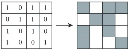
In a fragment-type structure, design space is dispersed into cells assigned with “1” or “0”, where cells assigned with “1” are to be metalized, as shown in Fig. 2. The distribution of “1” and “0” forms a two-dimensional (2D) 0/1 design matrix and can be used for optimization design, such as isolation, gain, beam pattern, bandwidth in [14].
1 0 0 1
1 0 1 0
3.2. Simulation of the Fragment-Type Structure Antenna by Using FDTD
This paper focuses on the microstrip antenna with a fragment-type structure as shown in Fig. 3, which is printed on a Duroid 5880 substrate (15.6 mm×33.6 mm×0.794 mm) with relative dielectric constant of 2.2. The antenna consists of a rectangular patch (L1 ×L2 = 16.0 mm×12 mm) and a microstrip feedline (L3×L4 = 2.40 mm×16.00 mm), where the distance between the feedline and the edge of the patch is L5 = 2.00 mm. The only difference between this structure and the one in [15] is that we take a fragmented discretization for the rectangular radiation patch.
1
L
2
L
3 L
1
W
2 W 3
W
5 L
4 L
Figure 3. Antenna configuration.
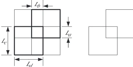
This paper selects Δx = 0.2 mm, Δy = 0.2 mm, Δz = 0.1985 mm, and time interval is set as Δt= 0.0331 ps according to the stability conditions. The simulated antennas all have the same spatial step and time interval. Therefore, the rectangular radiation patch can be divided into 60Δx×80Δy cells, and the distances between the edge of the patch and the edge of the substrate areW1 =W2 = 8Δx and W3 = 8Δy, respectively. The dimensions of the feedline are L3 = 12Δx and L4 = 80Δy. In this design, the size of each metallic element isLc×Ld. The sub-patches overlap with the size ofLa×Lb to
ensure electrical contact in such constellations in fabricated antenna [16]. The overlapped elements are shown in Fig. 4. It shall be noted that different cell sizes and overlapping sizes have certain influence on the electrical performance of the fragment-type antenna.
a
L b
L
c
L
d
L
Figure 4. Geometry of the overlapping element.
4. SIMULATION RESULTS
4.1. Different Cell Sizes
Firstly, the rectangular patch can be divided into 3×4 cells. The dimensions of each element are Lc = 20Δx andLd= 20Δy, and the size of the overlapping cell is La×Lb= Δx×Δy. The simulation
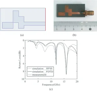
is performed for 10000 time steps. Fig. 5(a) shows a fragment-type antenna generated randomly. The prototype of this design is fabricated as shown in Fig. 5(b), and the simulated and measured results are illustrated in Fig. 5(c). From Fig. 5(c), it is clearly observed that agreement between numerical results is good. The slight difference between the simulated and measured results is believed to be caused by the fabrication and measurement error.
(a) (b)
(c)
Figure 5. Simulated and measured results of antenna divided into 3×4 cells. (a) Antenna structure, (b) photograph of the fabricated antenna, and (c) comparison of numerical results.
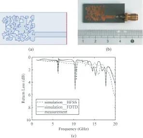
Secondly, the rectangular patch is divided into 15×20 cells. The dimensions of each element are Lc = 4Δx and Ld = 4Δy, and the size of overlapping cell is La×Lb = Δx×Δy, as time steps shall
be set as 10000. Fig. 6(a) provides a set of design model generated randomly. The prototype of this design is fabricated as shown in Fig. 6(b), and the numerical results are shown in Fig. 6(c). At this point, compared with the simulated result which is realized by means of the simulation of HFSS, slight frequency offset may exist in the numerical result realized by using FDTD. However, they are both in a similar trend. The slight difference between the simulated and measured results is believed to be caused by the fabrication and measurement error.
(a) (b)
(c)
Figure 6. Simulated and measured results of antenna divided into 15×20 cells. (a) Antenna structure, (b) photograph of the fabricated antenna, and (c) comparison of numerical results.
(a) (b)
(c)
Seen from the simulated results of above three antenna structures with different cell sizes, we can find that the fewer the cells are, the higher the precision is. Both of the simulated results obtained through FDTD and HFSS have certain errors, because
1) there are many irregular structures and parasitic elements in the fragment-type structures, which may cause serious current oscillation, so that energy cannot be radiated or reflected completely within finite time steps,
2) numerical errors from the simulation of FDTD, such as the exclusion of dielectric and conductor loss in the FDTD calculation. This will cause the calculatedS parameters shifting up at the higher frequencies. Meanwhile, the modeling error occurs primarily in the inability to match all of the circuit dimensions, and
3) numerical errors from the simulation of HFSS, such as the size of air box and dielectric loss of the substrate.
Table 1 exhibits the computation cost corresponding to the above designs using HFSS and FDTD. It is demonstrated that the high efficiency of the simulation by using FDTD is obvious when design matrix is large enough, which is useful for practical engineering applications.
Table 1. Comparison of time consumption. (Units: minute).
Design HFSS FDTD
Model Calculation Total time Total time
I 4.5 0.7 5.2 4.8
II 5.2 1.2 6.4 5.2
III 7.1 3.2 10.3 5.6
4.2. Different Overlapping Sizes
The influence of the different overlapping sizes is discussed in this section. The antenna structure with the radiation patch divided into 3×4 cells in Section 3.1 is used for comparison. The simulated results under the three circumstances are presented in Fig. 8. As can be seen, in this antenna structure, when the size of the overlapping cell is La×Lb = 3Δx×3Δy, compared with the simulated result realized by means of the simulation of HFSS, the numerical result realized by using FDTD is the most consistent. Therefore, it is concluded that different overlapping sizes will affect the accuracy of the numerical simulation. Therefore, in the practical engineering application, the overlapping size is of certain research significance.
5. CONCLUSIONS
The return loss of the fragment-type structure by using FDTD is calculated in this paper. The numerical results of the fragment-type antenna structures with different cell sizes and overlapping sizes are discussed. The validity of the numerical simulation of the fragment-type antenna by using FDTD is verified through the comparison between the simulated and measured return losses. Meanwhile, its efficiency in terms of computation time shows great potential in engineering applications, especially when the design matrix is large enough.
ACKNOWLEDGMENT
This work was financially supported by the National Natural Science Foundation of the Jiangsu Higher Education Institutions of China (Grant No. 16KJB510006) and Natural Science Foundation of the Jiangsu Basic Research Program of China (Grant No. BK20150528).
REFERENCES
1. Choo, H. and H. Ling, “Design of broadband and dual-band microstrip antennas on a high-dielectric substrate using a genetic algorithm,” IEEE Transactions on Antennas and Propagation, Vol. 150, No. 3, 137–142, Jun. 2003.
2. Choo, H., A. Hutani, and L. C. Trintinalia, “Shape optimisation of broadband microstrip antennas using genetic algorithm,” IET Electronics Letters, Vol. 36, No. 25, 2057–2058, Dec. 2000.
3. Alatan, L., M. I. Aksun, and K. Leblebicioglu, “Use of computationally efficient method of moments in the optimization of printed antennas,”IEEE Transactions on Antennas and Propagation, Vol. 47, No. 4, 725–732, Apr. 1999.
4. Pringle, L. N., P. H. Harms, and S. P. Blalock, “A reconfigurable aperture antenna based on switched links between electrically small metallic patches,” IEEE Transactions on Antennas and Propagation, Vol. 52, No. 6, 1434–1445, Jun. 2004.
5. Soontornpipit, P., C. M. Furse, and C. C. You, “Miniaturized biocompatible microstrip antenna using genetic algorithm,” IEEE Transactions on Antennas and Propagation, Vol. 53, No. 6, 1939– 1945, Jun. 2005.
6. John, M. and M. J. Ammann, “Wideband printed monopole design using a genetic algorithm,”
IEEE Antennas &Wireless Propagation Letters, Vol. 6, No. 11, 447–449, Sep. 2007.
7. Ding, D. W. and G. Wang, “MOEA/D-GO for fragmented antenna design,” Progress In Electromagnetics Research, Vol. 33, 1–5, Oct. 2013.
8. John, M. and M. J. Ammann, “Design of a wide-band printed antenna using a genetic algorithm on an array of overlapping sub-patches,” IEEE International Workshop on Antenna Technology Small Antennas and Novel Metamaterials, 92–95, 2006.
9. Herscovici, N., J. Ginn, and T. Donisi, “A fragmented aperture-coupled microstrip antenna,”IEEE Antennas and Propagation Society International Symposium, 1–4, San Diego, Jul. 2008.
10. Jin, Z., H. Yang, and X. Tang, “Parameters and schemes selection in the optimization of the fragment-type tag antenna,” Third International Joint Conference on Computational Science and Optimization IEEE Computer Society, Vol. 2, 259–262, May 2010.
11. Goojo, K. and Y. C. Chung, “Optimization of UHF RFID tag antennas using a genetic algorithm,”
IEEE Antennas and Propagation Society International Symposium, 2087–2090, Jul. 9–14, 2006. 12. Jin, Z., H. Yang, X. Tang, and J. Mao, “Impedance analysis of the fragment-type tag antenna using
FDTD,”International Symposium on Antennas, IEEE Transactions on Antennas and Propagation, 260–262, Nov. 2008.
13. Cummer, S. A., “A simple, nearly perfectly matched layer for general electromagnetic media,”
14. Johnson, J. M. and Y. Rahmat-Samii, “Genetic algorithms and method of moments (GA/MOM) for the design of integrated antennas,” IEEE Transactions on Antennas and Propagation, Vol. 47, No. 10, 1606–1614, Oct. 1999.
15. Sheen, D. M., S. M. Ali, and M. D. Abouzahra, “Application of the three-dimensional finite-difference time-domain method to the analysis of planar microstrip circuits,” IEEE Transactions on Microwave Theory & Techniques, Vol. 8, No. 7, 849–857, Jun. 1990.
16. Merulla, E. J. and R. Bansal, “Optimized design and fabrication of a fragmented wire antenna,”