ABSTRACT
BULLOCK, NOAH WILLIAM. Digital Pulse Pileup Deconvolution with Cerium (III) Bromide Scintillator. (Under the direction of Dr. John Mattingly.)
Gamma-ray spectroscopy in high count rate applications can be challenging with inorganic scintillators, due to their typical characteristically slow scintillation light emission rates, which contributes to pulse pile up that is difficult to mitigate using analog pulse processing. A rela-tively new inorganic scintillator, cerium (III) bromide (CeBr3) has very fast timing for medium
resolution, room temperature spectroscopic applications. It has a density of 5.2 g/cm3and emits approximately 68,000 photons per MeV of energy deposited, which is nearly twice as bright as sodium iodide. Using a Scionix 38.1mm (diameter) × 38.1mm (long) CeBr3 detector which
exhibits good resolution (3.9% at 662 keV) and fast timing (17 ns scintillation decay time), the ability to collect gamma-ray spectra in high count rate environments is possible. Using an XIA PIXIE-500, 500 megasample per second, 12-bit digitizer to digitally sample the CeBr3detectors
anode signal, a deconvolution algorithm was developed that is able to deconvolve piled up pulses within nanoseconds of other pulses. Using an analytical model of the expected pulse shape to deconvolve overlapping digitized anode pulses, the algorithm was able to deconvolve pulses and maintain good resolution with little energy broadening in high count rate applications. Starting with a 5µCi137Cs source (gamma-rays incident on the detector ≈1.02×10³γ/s) at 5 inches we
© Copyright 2014 by Noah William Bullock
Digital Pulse Pileup Deconvolution with Cerium (III) Bromide Scintillator
by
Noah William Bullock
A thesis submitted to the Graduate Faculty of North Carolina State University
in partial fulfillment of the requirements for the Degree of
Master of Science
Nuclear Engineering
Raleigh, North Carolina
2014
APPROVED BY:
Dr. Wolfgang Hennig Dr. Robin Gardner
BIOGRAPHY
DEDICATION
I want to dedicate this work to all of my brothers and sisters that are in uniform, have served in uniform, or gave their lives while serving. Thank you for what you do, and have done for all of us. Hoo-Yah.
ACKNOWLEDGEMENTS
I want to thank my advisor, Dr. John Mattingly for his guidance and support throughout my graduate career and research. Thank you for giving me the tools to succeed and the knowledge to use those tools effectively.
I want to thank my thesis committee members, Dr. Wolfgang Hennig and Dr. Robin Gardner. Dr. Hennig’s insight and knowledge about the Pixie-500 was very important to utilize the equipment as efficiently and effectively as possible. Dr. Gardner’s wealth of knowledge in high count rate applications and pervious work in pulse piled up deconvolution algorithms was invaluable to this project.
I want to thank Jack Linkous and Kyle Weinfurther for all of their help with learning MATLAB and in code writing skills. I started this endeavor never having opened MATLAB before, but with their help I was able to utilize the software and become very proficient in its use.
I also want to thank Kelsey Reamer and Kalene Hanson for the characterization of our cerium (III) bromide and sodium iodide detectors, excellent work.
TABLE OF CONTENTS
LIST OF TABLES . . . vii
LIST OF FIGURES . . . .viii
Chapter 1 Introduction . . . 1
1.1 Motivation . . . 1
1.2 Prior Work in the Field . . . 3
1.3 Contributions of this Research . . . 5
Chapter 2 Theory. . . 7
2.1 Scintillation Detectors . . . 7
2.1.1 Thallium-Activated Sodium Iodide (NaI(Tl)) . . . 10
2.1.2 Cerium(III) Bromide (CeBr3) . . . 11
2.2 Electronics . . . 12
2.2.1 Analog Pulse Processing . . . 12
2.2.2 Digitizer . . . 13
2.3 Pulse Pileup . . . 14
2.4 Pulse Shape Modeling . . . 16
2.4.1 Double Exponential Pulse Shape Model . . . 16
2.4.2 Pulse Height Spectrum . . . 22
2.5 Floating Averaging Low Pass Filter . . . 22
2.6 Fitting Algorithm . . . 24
Chapter 3 Experimental Procedures and Methods . . . 26
3.1 Experimental Setup . . . 26
3.2 Sodium Iodide and Cerium Bromide Setup . . . 27
3.3 Pixie-500 Setup . . . 29
3.4 Baseline Subtracting Pulses . . . 31
3.5 Flat-Topped Pulses . . . 36
3.6 Identifying Maximum Pulse Amplitude and Time of Maximum Amplitude . . . . 38
3.7 Fitting of Trace Windows . . . 41
3.8 PHS Code . . . 52
Chapter 4 Development of Deconvolution Algorithm Analysis Method . . . 57
4.1 Baseline Values . . . 57
4.2 Constant Fraction Discriminator vs. Differentiator . . . 59
4.3 Pulse Template Fitting vs. Analytical Model Fitting . . . 61
4.4 Fitting of Analytical Model to NaI(Tl) Pulses . . . 64
4.5 Fitting of Analytical Model to CeBr3 Pulses . . . 68
4.6 Levenberg-Marquardt vs. Trust Region Reflective Algorithm . . . 74
Chapter 5 Results . . . 77
5.1 Results . . . 77
5.2 5µCi Calibration Source Spectra using NaI(Tl) . . . 78
5.3 5µCi Calibration Spectra on CeBr3 . . . 80
5.4 4mCi 137Cs on NaI(Tl) . . . 82
5.5 4mCi 137Cs on CeBr3. . . 88
Chapter 6 Conclusions. . . 94
References. . . 98
Appendices . . . .101
Appendix A Pixie-500 Settings . . . 102
Appendix B CeBr3 Characterization and PMT Data . . . 105
B.1 Hamamatsu R6231 PMT . . . 109
Appendix C NaI(Tl) Detector Characterization Data . . . 110
LIST OF TABLES
Table 3.1 Instruments and equipment used for this research. Equipment used in the CeBr3 system is annotated with the † superscript. Equipment used in both
systems is annotated with a †† superscript. . . 27 Table 3.2 Relative uncertainties for NaI(Tl) fit values. . . 45 Table 3.3 Relative uncertainties for CeBr3 fit values. . . 51
Table 3.4 Fit values for PHS calibration. Y corresponds to the charge collected and x is the channel number. . . 53
Table 4.1 Nocente Pulse Shape Model Fit Parameters for Fig.4.17 and Fig.4.18. Values annotated with a ∗ are constants. . . 72 Table 4.2 TRR pulse parameter constraints for NaI(Tl) and CeBr3. . . 74
Table 5.1 Approximate gamma-ray currents at different distances from a 4mCi 137Cs source seen by a 50.8mm (diameter)×50.8mm (long) detector and a 38.1mm (diameter)×38.1mm (long) detector. . . 78 Table 5.2 Number of trace windows containing single, double, and triple pulses per
window for the 4mCi137Cs runs with NaI. Distance here refers to the source-to-detector distance. . . 83 Table 5.3 NaI(Tl) fit and analog PHS’s FWHM and resolution at 662 keV with different
source strengths of 137Cs and varying source-to-detector distances. . . 87 Table 5.4 Number of trace windows containing single, double, and triple pulses per
window for the 4mCi 137Cs runs with CeBr3. . . 88
Table 5.5 CeBr3 fit and analog PHS’s FWHM and resolution at 662 keV with different
source strengths of 137Cs and varying source-to-detector distances. . . 93 Table B.1 Calibration sources and original activity. All of these sources original activities
were measured on February 15, 2013. . . 105 Table B.2 Energy vs. channel and resolution fit coefficients and their goodness of fit values.106 Table B.3 Intrinsic efficiency fit coefficients and goodness of fit value. . . 106
LIST OF FIGURES
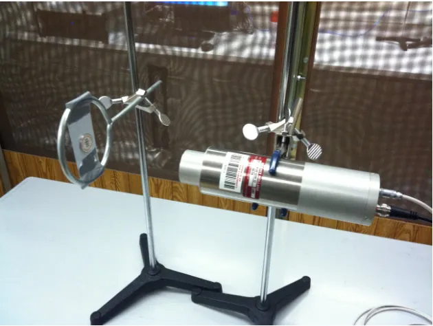
Figure 1.1 CeBr3 with calibration source setup for collecting PHS. . . 2
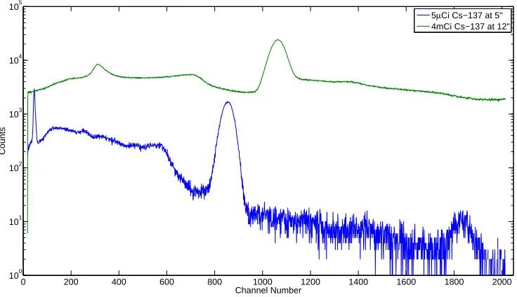
Figure 1.2 Comparison of analog PHS taken from a 38.1mm (diameter)×38.1mm (long) CeBr3 of a 5µCi 137Cs at 5 inches and a 4mCi 137Cs at 3 feet. Spectral distortion was shown, as well as a coincidence peak from the 662 keV gamma-rays (between channels 1600 to 1800). . . 3
Figure 2.1 NaI(Tl) inorganic scintillation crystal electron band structure. . . 8
Figure 2.2 CeBr3 inorganic scintillation crystal electron band structure. . . 8
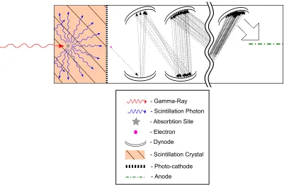
Figure 2.3 Gamma-ray detection through scintillation crystal. . . 10
Figure 2.4 Pulse width comparison between CeBr3 and NaI(Tl). . . 12
Figure 2.5 Analog pulse processing system with pulse shape at each stage. . . 13
Figure 2.6 Two piled pulse pulses from a NaI(Tl) detector. . . 15
Figure 2.7 Three piled pulse pulses from a NaI(Tl) detector. . . 15
Figure 2.8 Showing the effects of pulse pileup of a 137Cs in an NaI(Tl) analog pulse processing system. . . 16
Figure 2.9 Simplified parallel RC circuit diagram of the PMT. . . 17
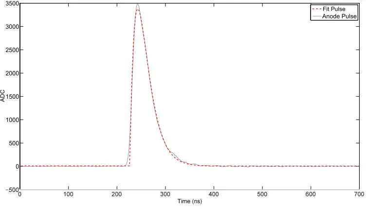
Figure 2.10 Single NaI(Tl) anode pulse fit to the analytical model described in Eq. 2.8. . 19
Figure 2.11 Single CeBr3 anode pulse fit to the analytical model described in Eq. 2.8. . . 19
Figure 2.12 NaI(Tl) trace window fit to the analytical model that describes the superpo-sition of multiple pulses as shown in Eq. 2.12. . . 21
Figure 2.13 CeBr3 trace window fit to the analytical model that describes the superpo-sition of multiple pulses as shown in Eq. 2.12. . . 21
Figure 2.14 NaI(Tl) anode pulse overlaid with the filtered anode pulse. . . 24
Figure 2.15 CeBr3 anode pulse overlaid with the filtered anode pulse. . . 24
Figure 3.1 NaI(Tl) nuclear pulse processing system setup. . . 28
Figure 3.2 CeBr3 nuclear pulse processing system setup. . . 28
Figure 3.3 2,500 ns NaI(Tl) trace window width. . . 30
Figure 3.4 700ns CeBr3 trace window width. . . 31
Figure 3.5 NaI(Tl) pulse with a pulse in the pre-trigger baseline region. . . 32
Figure 3.6 NaI(Tl) trace window with baseline regions shown. . . 33
Figure 3.7 Baseline determination checks. . . 34
Figure 3.8 CeBr3 trace window with baseline regions shown. . . 36
Figure 3.9 NaI(Tl) flat-top pulses. . . 37
Figure 3.10 CeBr3 flat-top pulses. . . 37
Figure 3.11 NaI(Tl) trace window with 2 anode pulses overlaid with the differentiated trace window. The dashed red lines show where the differentiated trace win-dow crosses zero. . . 39
Figure 3.13 τr vs. amplitude. Values used for estimating initial guesses for NaI(Tl) scin-tillation decay times based on pulse amplitude. . . 42 Figure 3.14 τf vs. amplitude. Values for estimating initial guesses for NaI(Tl) PMT decay
times based on pulse amplitude. . . 42 Figure 3.15 τr vs. amplitude. Values used for estimating initial guesses for CeBr3
scin-tillation decay times based on pulse amplitude. These are on a Log-Linear scale. . . 43 Figure 3.16 τf vs. amplitude. Values for estimating initial guesses for CeBr3 PMT decay
times based on pulse amplitude. These are on a Log-Linear scale. . . 43 Figure 3.17 Deconvolution algorithm flow chart. . . 44 Figure 3.18 NaI(Tl) relative uncertainties of the fit amplitude values above 1000 ADC. . 45 Figure 3.19 NaI(Tl) relative uncertainties of the fit amplitude values below 1000 ADC. . 46 Figure 3.20 NaI(Tl) relative uncertainties of the fit τr values with fit amplitudes above
1000 ADC. . . 46 Figure 3.21 NaI(Tl) relative uncertainties of the fit τr values with fit amplitudes below
1000 ADC. . . 47 Figure 3.22 NaI(Tl) relative uncertainties of the fit τf values with fit amplitudes above
1000 ADC. . . 47 Figure 3.23 NaI(Tl) relative uncertainties of the fit τf values with fit amplitudes below
1000 ADC. . . 48 Figure 3.24 CeBr3 relative uncertainties of the fit amplitude values above 1000 ADC.
These are on a log-linear scale. . . 48 Figure 3.25 CeBr3 relative uncertainties of the fit amplitude values below 1000 ADC.
These are on a log-linear scale. . . 49 Figure 3.26 CeBr3 relative uncertainties of the fit τr values with fit amplitudes above
1000 ADCs. These are on a log-linear scale. . . 49 Figure 3.27 CeBr3 relative uncertainties of the fit τr values with fit amplitudes below
1000 ADC. These are on a log-linear scale. . . 50 Figure 3.28 CeBr3 relative uncertainties of the fit τf values with fit amplitudes above
1000 ADC. These are on a log-linear scale. . . 50 Figure 3.29 CeBr3 relative uncertainties of the fit τf values with fit amplitudes below
1000 ADC. These are on a log-linear scale. . . 51 Figure 3.30 NaI(Tl) analog PHS compared to the fit PHS from a 5µCi60Co source. . . . 53
Figure 3.31 CeBr3 analog PHS compared to the fit PHS from a 5µCi 60Co source. . . 54
Figure 3.32 NaI(Tl) analog PHS compared to the fit PHS from a 5µCi22Na source. . . . 54 Figure 3.33 CeBr3 analog PHS compared to the fit PHS from a 5µCi 22Na source. . . 55
Figure 3.34 NaI(Tl) analog PHS compared to the fit PHS from a 5µCi137Cs source. . . . 55 Figure 3.35 CeBr3 analog PHS compared to the fit PHS from a 5µCi 137Cs source. . . 56
Figure 4.1 Deconvolution algorithm utilizing one baseline value for the entire trace win-dow. . . 58 Figure 4.2 Minimum separation time using a CFD on convolved pulses. . . 60 Figure 4.3 Left: NaI(Tl) analytical model of two pulses arriving 57 ns apart. Right:
Figure 4.4 Left: CeBr3 analytical model of two pulses arriving 20ns apart. Right:
Dif-ferentiated pulses crossing zero . . . 61
Figure 4.5 Comparison of the NaI(Tl) normalized template spectra taken from different sources and energy ranges. . . 62
Figure 4.6 A zoom on the trailing edge of the normalized template spectra derived from different radionuclei and their characteristic gamma-ray peaks. . . 62
Figure 4.7 Analytical model fit of a single pulse from NaI(Tl). . . 64
Figure 4.8 Analytical model fit of a double pulse from NaI(Tl). . . 65
Figure 4.9 Analytical model fit of a triple pulse from NaI(Tl). . . 66
Figure 4.10 Poor pulse fit from NaI(Tl) with 4mCi 137Cs at 1 foot. . . 66
Figure 4.11 Noise comparison of different amplitude NaI(Tl) pulses. Left: High amplitude pulse. Right: Lower amplitude pulse. . . 67
Figure 4.12 CeBr3 pulse overlaid with fit analytical model. The blue dashed boxes on the leading edge and the peak of the pulse show where the analytical model does not fit the pulse shape accurately. . . 69
Figure 4.13 Analytical model fit of a single pulse from CeBr3. . . 69
Figure 4.14 Analytical model fit of a double pulse from CeBr3. . . 70
Figure 4.15 Analytical model fit of a triple pulse from CeBr3. . . 70
Figure 4.16 Poor analytical model fit of a triple pulse from CeBr3. . . 71
Figure 4.17 Nocente pulse shape model fit of a single pulse from CeBr3. . . 73
Figure 4.18 Nocente pulse shape model fit of a single pulse from CeBr3. . . 73
Figure 4.19 Poor pulse fitting using the RMSE to check the goodness-of-fit. . . 76
Figure 5.1 Comparison of analog NaI(Tl) PHS to fit PHS of 5µCi 60Co at 5 inches. . . . 79
Figure 5.2 Comparison of analog NaI(Tl) PHS to fit PHS of 5µCi 22Na at 5 inches. . . . 79
Figure 5.3 Comparison of analog NaI(Tl) PHS to fit PHS of 5µCi 137Cs at 5 inches. . . 80
Figure 5.4 Comparison of analog CeBr3 PHS to fit PHS of 5µCi60Co at 5 inches. . . 81
Figure 5.5 Comparison of analog CeBr3 PHS to fit PHS of 5µCi22Na at 5 inches. . . 81
Figure 5.6 Comparison of analog CeBr3 PHS to fit PHS of 5µCi137Cs at 5 inches. . . . 82
Figure 5.7 Comparison of 10 minute analog NaI PHS to 5 minute fit PHS of 4mCi137Cs at 5 feet. . . 83
Figure 5.8 Comparison of 10 minute analog NaI PHS to 5 minute fit PHS of 4mCi137Cs at 3 feet. . . 84
Figure 5.9 Comparison of 10 minute analog NaI(Tl) PHS to 5 minute fit PHS of 4mCi 137Cs at 1 foot. . . 85
Figure 5.10 Comparison of analog NaI(Tl) PHS of 4mCi 137Cs at 5 feet, 3 feet, and 1 foot along with a 5µCi 137Cs at 5 inches. . . 86
Figure 5.11 Comparison of fit NaI(Tl) PHS of 4mCi 137Cs at 5 feet, 3 feet, and 1 foot. . . 87
Figure 5.12 Comparison of 10 minute analog CeBr3 PHS to fit PHS of 4mCi 137Cs at 5 feet. . . 89
Figure 5.13 Screen capture from the oscilloscope of the amplifier’s signal with the 4mCi 137Cs at a source-to-detector distance of 3 feet. . . 89
Figure 5.15 Screen capture from the oscilloscope of the pre-amplifier’s signal with the 4mCi 137Cs at a source-to-detector distance of 1 foot. . . 91
Figure 5.16 Screen capture from the oscilloscope of the amplifier’s signal with the 4mCi
137Cs at a source-to-detector distance of 1 foot. . . 91
Figure 5.17 Comparison of 10 minute analog CeBr3 PHS to fit PHS of 4mCi 137Cs at 1
foot. . . 92 Figure 5.18 Comparison of analog CeBr3 PHS of 4mCi137Cs at 5 feet, 3 feet, and 1 foot
along with a 5µCi137Cs at 5 inches. . . 92 Figure 5.19 Comparison of fit CeBr3 PHS of 4mCi137Cs at 5 feet, 3 feet, and 1 foot. . . 93
Figure B.1 CeBr3 characterization data. Upper Left: Energy vs. Channel curve. Upper
Right: Energy vs. Resolution curve. Bottom: Intrinsic efficiency curve. . . 106 Figure B.2 CeBr3 with calibration source setup to collect PHS to validate fitting
algo-rithms PHS. . . 107
Figure C.1 NaI(Tl) characterization data. Upper Left: Energy vs. Channel curve. Upper Right: Energy vs. Resolution curve. Bottom: Intrinsic efficiency curve. . . 111 Figure C.2 NaI(Tl) with calibration source setup to collect PHS for validation of the
Chapter 1
Introduction
1.1
Motivation
In the field of nuclear engineering and physics, precise and accurate gamma-ray spectra are essential for moving research and technology forward. In the realm of high count rate envi-ronments this becomes very difficult. Whether it is analog or digital pulse processing there are always limitations of the equipment and/or techniques. As count rates increase in a detec-tor, the probability of multiple gamma-ray interactions close in time increases. In analog pulse processing systems these manifest themselves in the spectrum as sum peaks or sometimes as gain shifts. These can be dealt with through pileup rejection circuitry, but in high count rate environments this circuitry can dramatically reduce the efficiency of the spectroscopic system. The goal of this work was to develop a deconvolution algorithm that uses nonlinear regression on a digitized photomultiplier tube (PMT) anode signal from a CeBr3 inorganic scintillator to
minimize spectral distortion in very high count rate environments. A thallium activated, sodium iodide (NaI(Tl)) inorganic scintillator was used as a baseline to evaluate CeBr3. This provided
a measurable demonstration of the capabilities of CeBr3 over a slow scintillator material, and
the effectiveness of digitizing the CeBr3 anode signal to create a pulse height spectrum (PHS)
Figure 1.1: CeBr3 with calibration source setup for collecting PHS.
spectral distortion caused by piled-up pulses in high count rate environments when standard multichannel analyzers (MCA) analog-to-digital (A/D) converters are used. Fig. 1.1 shows the setup of the 5µCi137Cs analog MCA experiment using our CeBr3 detector.
Fig. 1.2 shows the effects of these spectral distortions when the analog PHS of a 4mCi137Cs
was taken. The count rate seen by our CeBr3 detector using a 5µCi 137Cs at 5 inches was
approximately 1.02×10³ γs, where a 4mCi 137Cs, with a source-to-detector distance of 3 feet was approximately 1.61 ×10⁴ γs. The increased counts above the 662 keV peak (channel 850) is indicative of pulse pileup. The coincidence peak from two 662 keV gamma-rays interacting very close in time (between channels 1600 to 1800) is characteristic from PHS in high count rate environments with characteristic gamma-ray peaks emitted from a source. The backscatter peak seen around channel number 230 was due to the farther source-to-detector distance that created a higher number of backscattered gamma-rays that interacted inside the detector.
time-Figure 1.2: Comparison of analog PHS taken from a 38.1mm (diameter) × 38.1mm (long) CeBr3 of a 5µCi 137Cs at 5 inches and a 4mCi 137Cs at 3 feet. Spectral distortion was shown,
as well as a coincidence peak from the 662 keV gamma-rays (between channels 1600 to 1800).
dependent anode pulse shape can be used on digitized waveforms of the anode signal to decon-volve multiple overlapping pulses and mitigate these spectral distortions.
1.2
Prior Work in the Field
In the field of fusion reactors, gamma-rays with counting rates up to 106counts per second (cps) are starting to be used for diagnosis of reactions[1]. For these applications scintillation com-pounds with fast decay times are needed. For Nocente’s research a cerium activated, lanthanum bromide (LaBr3(Ce)) inorganic scintillator was used in conjunction with a 400 megasample per
second (MS/s). 14-bit digitizer that sampled the non-shaped, pre-amplified signal[1]. They pos-tulated that the pulse shapes do not change, only the arrival times of the pulses, amplitude of the pulses, and the baseline change. They used a model that fits the pulse shape, but only due to mathematical equation that contains values that have no physical properties of the detector or PMT (discussed later in Section 4.5). Nocente’s algorithm was able to measure gamma-ray spectra without degradation in the energy resolution up into the range of 2.6×10⁶ cps.
ap-plications. Sources of neutrons can be from the spontaneous fission of Califorium-252 (252Cf), Americium-Beryllium (AmBe)α-n reaction source, or deuterium (D-D) and deuterium-tritium (D-T) generators that can output up to 1015 neutrons per second[2]. 252Cf and AmBe sources constantly emit neutrons in a spectrum of energies, while D-D and D-T generators emit mono-energetic neutrons when turned on. These generators usually operate in a pulsed mode like in the work of H. Yang where the accelerator produced 5µs pulses with a maximum repetition rate of 600 Hz[3]. In homeland security, active neutron interrogation gamma-ray spec-troscopy is becoming more widely used for the detection of special nuclear material (SNM)[3]. These pulsed neutrons create bursts of gamma-rays due to interactions with nuclei in very short pulse periods. To accumulate accurate spectra from a sample, these gamma-rays need to arrive at times not overlapping with other gamma-ray interactions. This is usually not possible, so techniques need to be developed to deconvolve piled up pulses with detectors that are resolved enough to accurately identify important peaks associated with SNM and/or other important isotopes.
In work done by H. Yang in 2008, they used the premise that the recorded signal is a convolution of the input signal and system response function[3]. Once they determined the system response function, they could deconvolve individual pulses. Their analysis assumed that noise is negligible. Their work was able to digitize a cerium activated, lanthanum chloride (LaCl3(Ce)) anode signal with a 200 MS/s, 12-bit resolution digitizer at a rate greater than 106
cps with no dead time and no spectral shifts.
Another area of industry where high count rate environments are encountered is oil well logging. When boreholes are drilled, tools are lowered into the boreholes to test compositions on the surrounding environment. Conventional gamma-gamma density (GGD) logging tools use a 137Cs source to collect spectra, while newer neutron-gamma density (NGD) tools have been
neutron scattering and absorption can cause shifted spectra that create inaccurate spectral features due to pileup and gain shifts. The use of the NGD allows the deployment of this tool without the restrictions caused by the radioactive 137Cs due to the use of D-D or D-T generators. In work done by Weijun Guo, et al, they used the assumption that the scintillator decay time and PMT decay time are “somewhat” constant and can be expressed as the average of many measured results. They digitized the shaped, pre-amplified signal from a Lu2SiO5
(LSO) scintillator detector with a 10 MS/s, 8-bit resolution digitizer. Guo utilized an analytical model that was derived by assuming the PMT was a simple RC circuit. Guo used a differential pulse discriminator to initially determine amplitude and pulse arrival times, then he used a least-squares algorithm to fit the parameters to the pulse shape. Guo et al. used a Monte Carlo radiation transport code that assumed no dead time in the digitizer to show that this method was able to deconvolve piled-up pulses and maintain spectral resolution at 4×10⁶ cps[5].
1.3
Contributions of this Research
This research utilizes different aspects of the previous research to develop a new algorithm that will be more robust and able to deconvolve digitized pulses in high count rate environments accurately with the fast CeBr3 scintillator. Previous research in scintillator pulse shapes have
assumed that pulse shapes are constant and only vary in amplitude, arrival times, and baselines. Our approach uses an analytical model with multiple pulse parameters that will more accu-rately describe pulse shapes. It was shown that anode pulse shapes do in fact differ with pulse amplitudes, so treating scintillator and PMT decay times is needed for fitting a more accurate pulse shape. With slower scintillators it was found that individual pulses had two baselines, one before the pulse and one after the pulse. These additions allows for a more robust description of the pulse shape which will allow for more accurate determinations of the incoming gamma-ray energies.
• CeBr3 : Ideal for high count rate environments,
– Fast scintillation decay time (17ns),
– Good resolution (3.9% at 662 keV),
– No intrinsic radioactivity,
– Anode pulse widths≈ 150ns (NaI(Tl)≈1050ns),
• Directly digitizes the anode pulse,
– Bypasses any pre-amplification and amplification pulse shaping or gain shifts,
• 500 MS/s, 12-bit digitizer
– Voltage resolution in steps of 0.48mV,
– Timing resolution of 2ns,
• Varying scintillation & PMT decay times
• Pre- & post-trigger baselines
• Pulse detection by differentiation
– Can identify pulses separated by≈20 ns,
• Recursive fitting
– Re-examines residuals for “missed” pulses
which used the 500MHz, 12-bit digitizer on our CeBr3 detector. These techniques were applied
Chapter 2
Theory
2.1
Scintillation Detectors
Inorganic scintillation detectors have two important common requirements that make them suitable for detecting gamma-rays. These compounds typically have high photoelectric absorp-tion cross-secabsorp-tions, and the compound has to fluoresce in the visible spectrum (typically in the blue wavelengths ≈ 400nm) so these photons can be detected by a photocathode. To ensure photoelectric absorption of these gamma-rays, compounds should have at least one high atomic number (high-Z) constituent. To ensure the emission of a photon from the gamma-ray absorp-tion, compounds must have band levels that will allow electrons in the crystal to jump into the conduction band, then relax through an activator excited state that allow for the emission of photons able to be absorbed by the photocathode, before relaxing completely into the valence band again. This process is shown in Fig. 2.1.
CeBr3 is a self-activated scintillator[6]. Visible photons are emitted through a 5d to 4f level
transition in the cerium (Ce)[6]. (Discussed in Section 2.1.2). Fig. 2.2 shows the process for CeBr3.
{
Band Gap
Conduction Band
Valence Band
{
Thallium Excited States
Thallium Ground
State
Scintillation Photon
Figure 2.1: NaI(Tl) inorganic scintillation crystal electron band structure.
Conduction Band
Valence Band Cerium
States
Scintillation Photon
5d
4f
following energy deposition by incoming gamma-rays. Higher light yields correspond to a higher energy resolution of the crystal. Since radiation counting statistics follow a Poisson distribu-tion, its uncertainty is the square-root of the number of counts. This means, as NaI(Tl) emits approximately 38,000±195 photons/MeV while the more resolved CeBr3 emits 68,000±261
photons/MeV, NaI(Tl) has a higher proportional uncertainty in energies from the incoming gamma-rays which equates to a lower energy resolution. The relaxation time of the crystal’s fluorescent states controls the width of the light pulse. Scintillation compounds with fast re-laxation times correspond to fast scintillators and compounds with slower rere-laxation times are considered slow scintillators.
- Gamma-Ray
- Scintillation Photon
- Absorbtion Site
- Electron
- Dynode
- Scintillation Crystal
- Photo-cathode
- Anode
Figure 2.3: Gamma-ray detection through scintillation crystal.
2.1.1 Thallium-Activated Sodium Iodide (NaI(Tl))
pulse width of approximately 1050ns. This makes NaI(Tl) a good choice for medium resolution spectroscopy. NaI(Tl) was chosen as a baseline scintillator for these experiments.
One drawback of NaI(Tl) is that is has some longer lived phosphorescence states that cause an “afterglow,” and in high count rate environments these can cause the constant glowing of the crystal. The intermediate phosphorescence states of NaI(Tl) have a decay time of about 0.15s that contribute to about 9% of the photoelectric yield[9]. Another phenomenon associated with high count rate environments occurs in the PMT. As the amount of electrons increase from each dynode, it can cause a gain shift due to the potential difference at different dynodes[10]. Even though this detector is not suited for high count rate environments, it will be used as a baseline detector since most of its characteristics are very well documented. Appendix C shows the characterization of the NaI(Tl) detector used in these experiments. It also contains some of the characteristics of the ET Enterprises 9266B PMT coupled to it.
2.1.2 Cerium(III) Bromide (CeBr3)
Cerium (III) bromide is a self-activated crystal that has become more readily available and is showing impressive characteristics for room temperature medium resolution spectroscopy. CeBr3
has a relatively high average atomic number (Zavg = 40.75). The properties of this compound give it a Ce3+which is the “luminescence center for the scintillation process[8].” This compound emits photons that have a peak wavelength of 371nm due to Ce3+ 5d to 4f transition, emits approximately 68,000 photons per MeV (i.e. this is approximately twice as bright as NaI(Tl)), has an estimated rise time of 0.1 ns, and has a very fast scintillation decay time of 17 ns[8]. CeBr3 shows a non-linearity in light yield to deposited energy between 122 keV to 1274 keV
of about 4%[8]. Characterization of our 38.1mm (diameter) X 38.1mm (long) detector used for this research showed a resolution of 3.9% at 662 keV. Our detector showed a typical pulse width of approximately 150 ns. Fig. 2.4 shows the difference in pulse widths of a CeBr3 pulse
and NaI(Tl) pulse with similar amplitudes. Due to its resolution and fast timing, CeBr3 makes
0 200 400 600 800 1000 1200 1400 1600 1800 2000 500
0 500 1000 1500 2000 2500 3000 3500
Time (ns)
AD
C
CeBr3
NaI(Tl)
Figure 2.4: Pulse width comparison between CeBr3 and NaI(Tl).
makes it well suited for high count rate applications. Appendix B shows the characterization of the detector used in these experiments. It also contains some of the characteristics of the Hamamatsu R6231 PMT coupled to it.
2.2
Electronics
2.2.1 Analog Pulse Processing
Detector
2
1
Pre-Amplifier
3
Amplifier
4
ADC
5
6
Source
Figure 2.5: Analog pulse processing system with pulse shape at each stage.
depending on the scintillation decay time of the detector being used and the PMT decay time. At point 3, the pre-amplifier boosts the anode signal and has a shaping time long enough to allow complete charge collection (≈200µs). At point 4, the amplifier boosts the signal amplitude into the several-volt range and has varying shaping times in the microsecond range which gives the pulse an average width in the tens-of-microseconds range. At point 5, the multichannel analyzer (MCA) converts the peak analog signal voltage to a peak capture analog-to-digital conversion (ADC) value. The last stage at point 6, all of the digital ADC values are binned according to their value to build a pulse height spectrum (PHS).
2.2.2 Digitizer
exceed a threshold level. Once this threshold has been passed, the digitizer samples the signal for a specific window length (set by the user) before passing the data to the buffer. By digitizing the incoming anode signal from a detector, different methods can be employed to get the area under the pulse, which is proportional to the total charge collected from the PMT. These values are then binned, and a PHS can be built from all the digitized pulses.
This work was done using an XIA Pixie-500. It is a 12-bit A/D converter (displayed in units of ADC) with a 500 MS/s sampling rate[12]. The Pixie-500 has a dynamic range of 2V, and with 12-bit resolution can resolve input voltages in steps of 0.48mV[13]. This makes the Pixie-500 a very suitable tool to digital sample the anode pulse from fast detectors like CeBr3.
For more information about the Pixie-500 please consult Ref.[12, 13].
2.3
Pulse Pileup
In high count rate environments, a common problem encountered in analog pulse processing is pulse pileup. Pulse pileup occurs when multiple gamma-rays interact within the detector in a short time window that causes the anode signal to contain multiple pulses that are sent to the pre-amplifier. Fig. 2.6 shows two incoming pulses and Fig. 2.7 has three incoming pulses. The voltage pulse measured by the MCA would be the sum of the total voltages of all the pulses after amplification. Fig.2.8 clearly shows the effect to a PHS due to pulse pileup. The spectrum in blue was from a 5µCi137Cs (low count rate), and the green spectrum was from a 4mCi137Cs (high count rate). In the 4mCi spectrum a shifted 662 keV peak and high counts above the 662 keV peak show the effects of pulse-pileup in the detector.
0 500 1000 1500 2000 2500 200
0 200 400 600 800 1000
Time (ns)
AD
C
Figure 2.6: Two piled pulse pulses from a NaI(Tl) detector.
0 500 1000 1500 2000 2500
200 0 200 400 600 800 1000
Time (ns)
AD
C
0 200 400 600 800 1000 1200 1400 1600 1800 2000 100
101 102 103 104 105
Channel Number
Counts
5µCi Cs−137 at 5" 4mCi Cs−137 at 12"
Figure 2.8: Showing the effects of pulse pileup of a137Cs in an NaI(Tl) analog pulse processing system.
2.4
Pulse Shape Modeling
For the proper fitting of pulses to determine pulse characteristics, an analytical model was used. With an understanding of the dynamics of scintillation and electron multiplication in the PMT, an equation can be developed that describes the pulse shape needed for pulse fitting.
2.4.1 Double Exponential Pulse Shape Model
Since the PMT is a series of parallel resistors (R) and capacitors (C), a simple idealized parallel RC circuit can be used to derive the current at the anode as shown in Fig. 2.9.
Starting with this simple equation[6]:
i(t) =i0e−λrt, t >0 (2.1)
R C V(t) i(t)
iR(t) iC(t)
Figure 2.9: Simplified parallel RC circuit diagram of the PMT.
initial current. To get the total charge collected (Q), i(t) needs to be integrated:
Q=
Z ∞
0
i(t)dt→Q= i0 λr
, (2.2)
which now gives the value fori0, and Eq. 2.1 can be written as:
i(t) =λrQe−λrt. (2.3)
Since the current flowing from the anode is the sum of the current flowing through the capacitors and resistors, the total current is written as:
i(t) =iR+iC, (2.4)
and this can be re-written as:
i(t) =CdV(t) dt +
V(t)
R . (2.5)
λrQ C e
−λrt= dV(t)
dt + V(t)
RC . (2.6)
Eq.2.6 can now be solved with the initial condition at t= 0,V(0) = 0, which is:
V(t) =A λr λr−λf
(e−λft−e−λrt), (2.7)
where A = Q/C, λf = 1/τf, and τf = RC which is the PMT decay time. To be able to fit a
multiple pulses with different arrival times a Heaviside step function was added to the pulse shape model. Also, a pre- and post-trigger baseline was added to the pulse shape model shown in Eq.2.8:
V(t) =H(t)A λr λr−λf
(e−λft−e−λrt) + (1−H(t))B
−+H(t)B+, (2.8)
where B− is the pre-trigger baseline value, and B+ is the post-trigger baseline. H(t) is the
Heaviside step function:
H(t) = Z ∞ t δ(t)dt =
1 t≥0
0 t <0
(2.9)
whereδ(t) is the Dirac delta function. Since my research utilized MATLAB, it used a different form of the Heaviside step function shown in Eq. 2.10.
H(t) =
1 t >0
1/2 t= 0
0 t <0
(2.10)
0 500 1000 1500 2000 2500 500
0 500 1000 1500 2000 2500 3000 3500 4000 4500
Fit Pulse Anode Pulse
AD
C
Figure 2.10: Single NaI(Tl) anode pulse fit to the analytical model described in Eq. 2.8.
0 100 200 300 400 500 600 700
500 0 500 1000 1500 2000 2500 3000 3500
1st Pulse Anode Pulse Fit Pulse
AD
C
this analytical model’s fit is optimal, CeBr3 appears to have an exponential rise of the leading
edge of the anode pulse which is not fully described by our analytical model.
Since the purpose of this work is to be able to fit multiple pulses in one trace window, models need to be created to do this. This was done by the superposition of multiple pulses given by Eq.2.11:
Vn(t) =Hn(t−tn)An λrn
λrn −λfn
(e−λfn(t−tn)−e−λrn(t−tn)). (2.11)
When Eq. 2.11 is incorporated with the pre- and post-trigger baseline values it becomes Eq. 2.12:
V(t) = (1−H(t−t1))B−+H(t−t1)B++
N
X
n=1
Vn(t), (2.12)
whereN is the total number of pulses in a trace window. Now Eq.2.12 can fit multiple pulses per trace window and fit each pulses individual parameters. The pre- and post-trigger baseline is only evaluated from the time of the first pulse (t1). Fig.2.12 shows multiple pulses in a NaI(Tl)
0 500 1000 1500 2000 2500 200
0 200 400 600 800 1000 1200 1400 1600
1st Pulse 2nd Pulse Anode Pulse
AD
C
Figure 2.12: NaI(Tl) trace window fit to the analytical model that describes the superposition of multiple pulses as shown in Eq. 2.12.
0 50 100 150 200 250 300 350 400
500 0 500 1000 1500 2000 2500 3000 3500
1st Pulse 2nd Pulse Anode Pulse
AD
C
Figure 2.13: CeBr3 trace window fit to the analytical model that describes the superposition
2.4.2 Pulse Height Spectrum
The PHS is final result of using the fitting algorithm to deconvolve multiple pulses in a trace window. In high count rate environments analog nuclear pulse processing systems can use rejection circuitry to omit piled up pulses. Without this rejection circuitry being used piled up pulses can cause shifts in the spectra and accidental coincidence sum peaks. In some cases the count rate can become so high that pulse pileup dominates the spectrum and destroys the accuracy of the spectrum.
By digitizing the anode pulse and using fitting algorithms, pulse parameters can be ex-tracted and utilized to build a PHS that eliminates pileup. Having an analytical model of these pulses, degradation of the spectra can be mitigated by correcting spectrum distortion through deconvolution of piled up pulses. Since the PHS is a histogram of the charge collected (Q) values from each pulse, Eq.2.8 can be integrated to solve for Q:
Qn=
Z ∞
0
Vn(t) R dt∝
Z ∞
0
Vn(t)dt, (2.13)
which becomes:
Qn∝An λrn
λrn−λfn
( 1 λfn
− 1
λrn
), (2.14)
Qn∝Anτfn. (2.15)
From Eq.2.15 a PHS can be built from the individual pulses fit amplitudes (An) and PMT decay times (τfn).
2.5
Floating Averaging Low Pass Filter
phe-nomenon will usually just manifest itself as an increased baseline that shifts the spectra a small amount. Due to the digitizer taking the anode pulse directly, this noise can be more problematic and give false triggers. Because of this, a filter was written to minimize this effect. This filter is shown below:
Y(t) = 1 2T+ 1
t+T
X
i=t−T
y(i), (2.16)
whereY(t) is the filtered pulse value, y(i) is the original pulse value,tis the time step value in the trace, andT is the half-width of the filter. Fig. 2.14 shows a digitized NaI(Tl) anode pulse with the filtered pulse overlaid. Due to the noise in the NaI(Tl) we used a 41 point (T = 20) floating average filter. Fig.2.15 shows a digitized CeBr3 anode pulse overlaid with the filtered
pulse. The CeBr3 was not very noisy, but we opted to still use a 21 point (T = 10) floating
0 500 1000 1500 2000 2500 500
0 500 1000 1500 2000 2500 3000 3500 4000
Time (ns)
AD
C
Anode Pulse Filtered Pulse
Figure 2.14: NaI(Tl) anode pulse overlaid with the filtered anode pulse.
0 100 200 300 400 500 600 700
1000 0 1000 2000 3000 4000 5000 6000
Time (ns)
AD
C
Anode Pulse Filtered Pulse
Figure 2.15: CeBr3 anode pulse overlaid with the filtered anode pulse.
2.6
Fitting Algorithm
Chapter 3
Experimental Procedures and
Methods
3.1
Experimental Setup
Table 3.1: Instruments and equipment used for this research. Equipment used in the CeBr3
system is annotated with the†superscript. Equipment used in both systems is annotated with a †† superscript.
Instrument Manufacturer Model Number
High Voltage Power Supply ORTEC 556
Low Voltage Power Supply† BK Precision 1550
38.1mm ×38.1mm CeBr3† Scionix 38B38/2M-HV-CEBR-X2
50.8mm ×50.8mm NaI(Tl) ORTEC 905-3
Pre-Amplifier† Canberra 2005
Pre-Amplifier ORTEC 276
Amplifier†† ORTEC 572A
NIM Bin†† ORTEC 4001A
2K Multi-Channel Analyzer†† ORTEC EASY-MCA-2K
Fast Waveform Digitizer†† XIA-National Instruments Pixie - 500
Oscilliscope†† Tektronix DPO2012
3.2
Sodium Iodide and Cerium Bromide Setup
To create a potential difference at each dynode and the anode in the PMT, a high voltage (HV) power supply was used. It is important to correctly set the HV to a level that provides enough electron multiplication for sufficient current to pass through the anode. Increasing the HV causes higher current pulses which will shift the PHS to the right. Having the HV setting too low may not provide enough potential in the PMT for sufficient electron multiplication and current flowing from the anode will be very small.
The NaI(Tl) detector used a standard adjustable HV power supply connected directly to the detector. The CeBr3 detector used a low voltage (LV) power supply connected to a
self-contained HV power supply that could be adjusted on the detector. The LV power supply fed 5V to the HV power supply and a simple potentiometer to adjust the HV settings.
Detector HV Power
Pre-Amp Amplifier MCA Computer
Source
Analog NaI(Tl) Nuclear Pulse Processing System
Source
Digitizer
Digitial NaI(Tl) Nuclear Pulse Processing System
Pre-Amplifier Power
NIM Bin
HV Power
Detector
Figure 3.1: NaI(Tl) nuclear pulse processing system setup.
Detector w/ HV Power
LV Power
Pre-Amp Amplifier MCA Computer
Source
Analog CeBr
3
Nuclear Pulse Processing System
LV Power
Source
Digitizer
Digitial CeBr
3
Nuclear Pulse Processing System
Pre-Amplifier Power
NIM Bin
Detector w/ HV Power
detector, and an HV setting of 850V for CeBr3. Since our digitizer is sampling from the anode
with no amplification, sufficient electron multiplication from the PMT must occur. Since typical anode pulses are in the millivolt range, the HV of the detectors was kept at 1000V to maximize current, but not create overly high current pulses when we directly digitized the anode signal.
3.3
Pixie-500 Setup
This section of the research was not meant to completely resolve the best settings for the Pixie-500, merely to obtain values that allow the research to be completed correctly so the fitting algorithm can be built and tested. Commentary about the Pixie-500 and its settings can be found in Appendix A. Some of these settings were used from pulse shape discrimination research done by Zachary Bailey[20].
The Pixie-500 uses a leading edge trigger to capture incoming waveforms. Since each detector is different, the leading edge thresholds must be set for each detector. In noisy detectors stray signals may cross the leading edge trigger in the digitizer and cause it to digitize noise more than actual gamma ray scintillation events. The NaI(Tl) detector used for these experiments needed an leading edge threshold setting of 200 ADC channels to mitigate this noise. The CeBr3
detector only needed a leading edge threshold setting of 25 ADC channels to accomplish this. The Pixie-500 has internal memory called a “buffer” where it stores digitized waveforms. It can store a maximum of 8K words of data in a buffer before it is considered full. A “spill” is a term used for when the data stored in the buffer is transferred to the external memory. The Pixie-500 has 3 modes for “List Mode Run,” the setting used for these experiments was 32 events per buffer. This means a maximum of 32 events were captured in one buffer, and only after 32 events were captured or the buffer was full did the data in the buffer transfer to the external memory card.
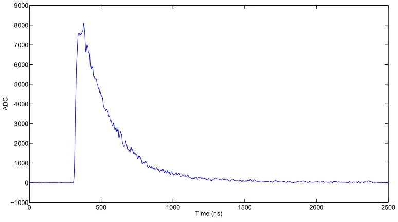
The trace window length was also something that varied for each detector. NaI(Tl) has a longer scintillation decay time and PMT decay time and needed a longer trace window to capture the full waveform. The appropriate setting found for our NaI(Tl) detector used a total trace window length of 2,500 ns with a 200 ns pre-trigger trace as shown in Fig.3.3.
0 500 1000 1500 2000 2500
1000 0 1000 2000 3000 4000 5000 6000 7000 8000 9000
Time (ns)
AD
C
Figure 3.3: 2,500 ns NaI(Tl) trace window width.
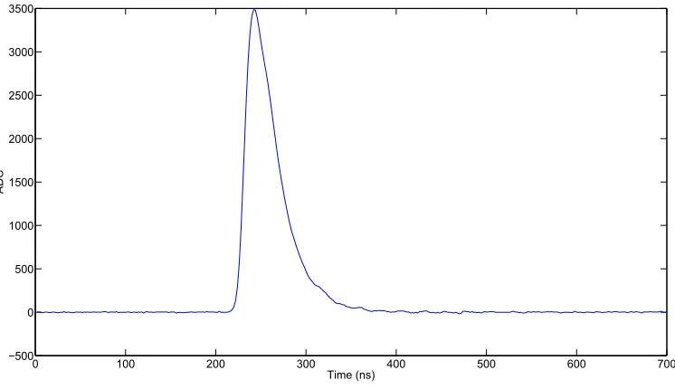
For CeBr3 the total trace window length was 700 ns with a 200 ns pre-trigger trace as
0 100 200 300 400 500 600 700 500
0 500 1000 1500 2000 2500 3000 3500
Time (ns)
AD
C
Figure 3.4: 700ns CeBr3 trace window width.
3.4
Baseline Subtracting Pulses
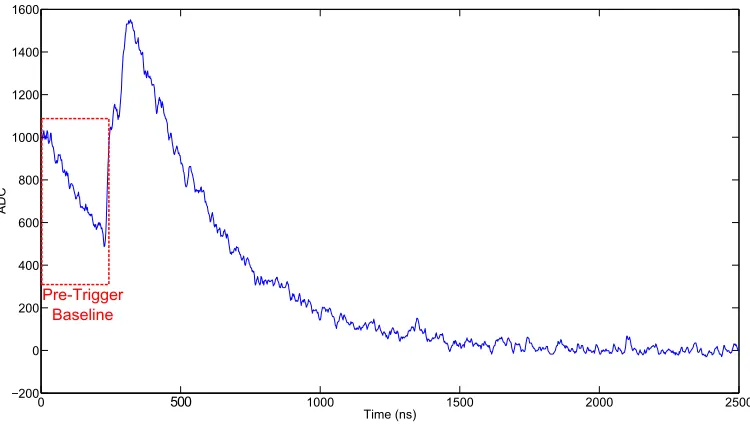
Although the Pixie-500 does calculate an average baseline when digitizing the anode pulse, a more rigorous algorithm was developed to accurately set the baseline of the trace windows as close to zero as possible. In low count rate environments it can be as simple as averaging the baseline of the pre-trigger trace and then subtracting that value from the entire window. This breaks down when an arriving pulse has a pulse in the pre-trigger trace as shown in Fig. 3.5.
Due to this phenomenon, the fitting algorithm was modified to fit a pre- and post-trigger baseline which the algorithm averages a pre-trigger and post-trigger baseline value.
For NaI(Tl), the data showed that it took a long time before the tail of the pulse decayed back to the pre-trigger baseline levels. The trace windows needed to be kept long enough to capture the entire anode pulse and not clip the tail. This phenomenon was very evident in the NaI(Tl) detector, but was not as evident in the CeBr3 detector due to its short pulse decay
0 500 1000 1500 2000 2500 200
0 200 400 600 800 1000 1200 1400 1600
Time (ns)
AD
C
Pre-Trigger Baseline
Figure 3.5: NaI(Tl) pulse with a pulse in the pre-trigger baseline region.
100 digitized samples in the trace window, and the post-trigger baseline by the mean of the last 100 digitized samples in the trace window. Due to the possibility of multiple pulses arriving in the pre- and post-trigger baseline regions, checks were used to calculate the most accurate baseline values from the trace window. Fig. 3.6 shows the regions where the baseline values are extracted from in NaI(Tl) pulse windows.
The general checks for determining the baselines are shown in Fig. 3.7. The specific base-line value checks for each detector are described below. As a note, the determination of what constituted a “good” initial guess of baseline values was done through experimentation. Values above 10 ADC most likely corresponded to a pulse in the trace in those regions. The ideal pre-and post-trigger baselines should be 0 ADC. So by setting a threshold less than 1 ADC for “good” initial guesses of pre- and post-trigger baseline values yielded better results for initial guesses.
0 500 1000 1500 2000 2500 1000 0 1000 2000 3000 4000 5000 6000 7000 8000 9000 Time (ns) AD C s Post-Trigger Baseline Pre-Trigger Baseline Secondary Post-Trigger Baseline Secondary Pre-Trigger Baseline
Figure 3.6: NaI(Tl) trace window with baseline regions shown.
1. If pre-trigger baseline value <1 ADC
(a) The pre-trigger baseline value is subtracted from the entire trace window
(b) Pre- and post-trigger baseline values are recalculated for initial guesses for fit pa-rameters
(c) Pre-trigger baseline value is accepted for initial guess
(d) If post-trigger baseline value<10 ADC
• Post-trigger baseline value is accepted for initial guess
(e) If post-trigger baseline value>10 ADC
i. Recalculate post-trigger baseline in 1800 ns to 2000 ns secondary post-trigger region
ii. If post-trigger baseline value<10 ADC
Starting Point
Pre-Trigger Baselline Check If 1 ADCs
1 -Subtract initial pre-trigger from trace window 2. Recalculate pre- & post-trigger baselines
Post-Trigger Baseline Check
If > 10 ADCs
Recalculate post-trigger baseline from secondary region
Secondary Post-Trigger Baseline Check
If > 10 ADCs
Set post-trigger baseline value to
0 ADCs
Guessed post-trigger baseline value If 10 ADCs
Guessed pre-trigger baseline value
If > 1 ADCs
Post-Trigger Baseline Check If 1 ADCs
1 -Subtract initial post-trigger from trace window 2. Recalculate pre- & post-trigger baselines
Set pre-trigger baseline value to
0 ADCs Pre-Trigger
Baseline Check
If > 10 ADCs
Recalculate pre-trigger baseline from secondary region
Secondary Pre-Trigger Baseline
Check
If > 10 ADCs
If 10 ADCs Guessed pre-trigger baseline value Guessed post-trigger baseline value If 10 ADCs
If > 1 ADCs
iii. If post-trigger baseline value >10 ADC
• Post-trigger baseline value is set to 0 ADCs for initial guess
2. If pre-trigger baseline value >1 ADC and post-trigger baseline value<1 ADC
(a) The post-trigger baseline value is subtracted from the entire trace window
(b) Pre- and post-trigger baseline values are recalculated for initial guesses for fit pa-rameters
(c) Post-trigger baseline value is accepted for initial guess
(d) If pre-trigger baseline value <10 ADC
• Pre-trigger baseline is accepted for initial guess
(e) If pre-trigger baseline value >10 ADC
i. Recalculate pre-trigger baseline in 100nsto 200nssecondary pre-trigger region
A. If pre-trigger baseline value <10 ADC
• Pre-trigger baseline is accepted for initial guess
B. If pre-trigger baseline value >10 ADC
• Pre-trigger baseline value = 0 ADC
3. If pre- and post-trigger baseline values are >1 ADC
• Pre- and post-trigger baseline values set to 0 ADC for initial guess
For CeBr3 the algorithm works exactly the same, only the regions for the secondary
0 100 200 300 400 500 600 700 500
0 500 1000 1500 2000 2500 3000 3500
Time (ns)
AD
C
s
Pre-Trigger
Baseline Post-TriggerBaseline
Secondary Post-Trigger
Baseline Secondary
Pre-Trigger Baseline
Figure 3.8: CeBr3 trace window with baseline regions shown.
3.5
Flat-Topped Pulses
The Pixie-500 has an internal oscilloscope that can be used to set the gain offsets of the incoming channels. The ADC has an input range of 2V and this gain adjustment tunes the dynamic range of the channel. Due to flat-topping, there can be some saturation of high current pulses. From experimentation the NaI(Tl) and CeBr3 both had this floating “flat-top” to these high current
pulses as shown in Fig.3.9 and Fig 3.10.
440 460 480 500 520 540 560 580 1.38
1.4 1.42 1.44 1.46 1.48 1.5
x 104
Time (ns)
AD
C
Figure 3.9: NaI(Tl) flat-top pulses.
475 480 485 490 495 500 505
1.45 1.455 1.46 1.465 1.47 1.475 1.48
x 104
AD
C
Time (ns)
3.6
Identifying Maximum Pulse Amplitude and Time of
Max-imum Amplitude
The next two initial guess values that need to be determined to pass to the fitting algorithm are the maximum amplitude of the pulse and the time that the maximum amplitude arrived. Since the NaI(Tl) detector used for these experiments had a lot of signal noise, a floating average low pass filter was applied to all the trace windows to smooth out the digitized anode signal; a 41 point floating average was used. CeBr3 had little to no noticeable noise in the
traces, so a 21 point floating average was used to smooth out its data. These filtered pulses were then differentiated to find the maximum amplitudes and times. Since differentiating these trace windows will show a zero crossing at local maxima and minima, a threshold trigger was used to start looking for zero crossings in the derivatives of the trace windows. Due to the floating point averaging filter, false maxima were shown in the differentiated trace windows at two specific points. Since NaI(Tl) used a 41 point floating average, the starting point was 21 digitized sample into the trace window, and ended 21 digitized samples before the end of the window. In CeBr3 the first and last 10 digitized samples were omitted due to this floating
point averaging filter. From experimentation a differentiated pulse trigger level of 19 ADC was used to look for pulses in NaI(Tl), and 6 ADC in CeBr3. Once a value in the trace goes above
the trigger threshold, it starts to look for the data point value to go below zero. Once below zero, the digitized sample value was recorded, and the algorithm continued searching the rest of the window for values above the trigger level. Fig.3.11 shows a NaI(Tl) anode pulse with the differentiated pulse overlaid with the zero crossings marked. Fig.3.12 shows a CeBr3 anode
pulse with the differentiated pulse overlaid with the zero crossings marked.
0 500 1000 1500 2000 2500 5000
0 5000
AD
C
0 500 1000 1500 2000 2500100
0 100
Time (ns)
AD
C
Anode Pulse Differentiated Pulse
Zero Crossings
Figure 3.11: NaI(Tl) trace window with 2 anode pulses overlaid with the differentiated trace window. The dashed red lines show where the differentiated trace window crosses zero.
0 100 200 300 400 500 600 700 5000
0 5000 10000
AD
C
0 100 200 300 400 500 600 700200
0 200 400
Time (ns)
AD
C
Anode Pulse Differentiated Pulse
Zero Crossings
Figure 3.12: CeBr3 trace window with 2 anode pulses overlaid with the differentiated trace
3.7
Fitting of Trace Windows
To improve the efficiency of fitting, a correction to the initially guessed amplitudes was needed. Since the stored amplitude parameter is convolved with τr and τf values (see Eq. 2.8) from the analytical model, a correction factor was applied to the initial guess of the amplitude to make the initial guess value closer to the real amplitude value. Plotting the originally guessed amplitudes to the fit amplitudes, it was found that they all followed a nearly linear trend. Due to this, all the amplitudes for NaI(Tl) were multiplied by 1.3533, and CeBr3 by 1.7970.
It was found that the zero crossing times also needed to be corrected to pass better initial guesses for pulse arrival times to the fitter. It was found for NaI(Tl) that the average zero crossing times were approximately 60nsahead of the pulse arrival times. For CeBr3 the average
zero crossing times were approximately 25ns ahead of the fit pulse arrival times. So each zero crossing time had its pulse arrival time adjustment subtracted from it to give us our pulse arrive time initial guesses.
The next step after these corrections were made was to calculate initial guesses for the scintillator decay time (τr) and PMT decay time (τf). This was done by correlating single fit pulse amplitudes to fit pulse scintillation and PMT decay times. These values were then used to linearly interpolate guessed amplitudes to reasonable guessedτr and τf values. Now all the required fit initial guesses have been determined, and fitting can be started on the trace windows.
Fig.3.13 and Fig. 3.14 show the values used to obtain the initial guesses for the τr and τf for NaI(Tl). Fig.3.15 and Fig. 3.16 show the values used to obtain the initial guesses for theτr and τf for CeBr3.
0 2000 4000 6000 8000 10000 12000 14000 16000 18000 10
12 14 16 18 20 22
Amplitude ADC Values
Scintill
ation Decay Ti
me (ns)
NaI Fit Amplitudes vs. Fit Rise Times
Figure 3.13: τrvs. amplitude. Values used for estimating initial guesses for NaI(Tl) scintillation decay times based on pulse amplitude.
0 2000 4000 6000 8000 10000 12000 14000 16000 18000 170
180 190 200 210 220 230 240 250 260
Amplitude ADC Values
PMT De
cay Time (
ns)
NaI Fit Amplitudes vs. Fit Fall Times
0 0.5 1 1.5 2 2.5 3 3.5 4 x 10⁴ 9
10 11 12 13 14 15 16 17 18
Amplitude ADC Values
Scintill
ation Decay Ti
me (ns)
CeBr
3Fit Amplitudes vs. Fit Rise Times
Figure 3.15: τr vs. amplitude. Values used for estimating initial guesses for CeBr3 scintillation
decay times based on pulse amplitude. These are on a Log-Linear scale.
0 0.5 1 1.5 2 2.5 3 3.5 4
x 104 16
18 20 22 24 26 28
Amplitude ADC Values
PMT De
cay Time (
ns)
CeBr3Fit Amplitudes vs. Fit Fall Times
Figure 3.16: τf vs. amplitude. Values for estimating initial guesses for CeBr3PMT decay times
Fitting Algorithm Guessed Parameters Fit Parameters Relative Uncertainty Check of Fit:
Amplitude, r, f, t0
Fit Parameters Stored for PHS Analysis
Pass
Fail
Fit pulse is subtracted from original trace window Residual trace window
goes through floating average low pass filter
Number of pulses in residual trace window are identified, and pulse
parameters determined
Update: number of pulses in original trace window Sort all guessed parameters by ascending arrvial time
Guessed Parameters
Number of pulses in trace window matched with correct
fitting model
Starting Point
Figure 3.17: Deconvolution algorithm flow chart.
the fit values uncertainty divided by the fit value.
0 0.005 0.01 0.015 0.02 0.025 0.03 0.035 0.04 0
1 2 3 4 5 6
7x 10
4
σA/A
Frequency
Figure 3.18: NaI(Tl) relative uncertainties of the fit amplitude values above 1000 ADC.
Table 3.2: Relative uncertainties for NaI(Tl) fit values.
Rel. Uncertainties ≤1000 ADC >1000 ADC
σamp/A 2 0.03
στr/τr 2 0.1
στf/τf 2 0.07
shows the relative uncertainties of theτr fit parameter with pulse amplitudes above 1000 ADC, and Fig. 3.21 shows the relative uncertainties of theτrfit parameter with pulse amplitudes below 1000 ADC. Fig. 3.22 shows the relative uncertainties of the τf fit parameter with amplitudes above 1000 ADC. Fig. 3.23 shows the relative uncertainties of the τf fit parameter with pulse amplitudes below 1000 ADC. The refitting threshold values for NaI(Tl) are shown in Table 3.2. It was found these values accepted enough well fit pulses while omitting poorly fit ones.
0 0.1 0.2 0.3 0.4 0.5 0.6 0.7 0.8 0.9 1 0
500 1000 1500 2000 2500 3000 3500 4000 4500 5000
σA/A
Frequency
Figure 3.19: NaI(Tl) relative uncertainties of the fit amplitude values below 1000 ADC.
0 0.02 0.04 0.06 0.08 0.1 0.12 0.14
0 500 1000 1500 2000 2500 3000 3500 4000 4500
στ
r
/τr
Frequency
0 0.1 0.2 0.3 0.4 0.5 0.6 0.7 0.8 0.9 1 0
500 1000 1500 2000 2500 3000
στ
r
/τr
Frequency
Figure 3.21: NaI(Tl) relative uncertainties of the fit τr values with fit amplitudes below 1000 ADC.
0 0.005 0.01 0.015 0.02 0.025 0.03 0.035 0.04 0.045 0.05
0 0.5 1 1.5 2
2.5x 10
4
στ
f
/τf
Frequency
0 0.1 0.2 0.3 0.4 0.5 0.6 0.7 0.8 0.9 1 0
500 1000 1500 2000 2500 3000
στ
f
/τf
Frequency
Figure 3.23: NaI(Tl) relative uncertainties of the fitτf values with fit amplitudes below 1000 ADC.
0 20 40 60 80 100 120 140 160 180 200
100 101 102 103 104
A/A
F
re
q
u
e
n
cy
Figure 3.24: CeBr3 relative uncertainties of the fit amplitude values above 1000 ADC. These
0 20 40 60 80 100 120 140 160 180 200 100
101 102 103 104
A/A
F
re
q
u
e
n
cy
Figure 3.25: CeBr3 relative uncertainties of the fit amplitude values below 1000 ADC. These
are on a log-linear scale.
0 20 40 60 80 100 120 140 160 180 200
100 101 102 103 104 105
r
/r
F
re
q
u
e
n
cy
0 20 40 60 80 100 120 140 160 180 200 100
101 102 103 104
r
/r
F
re
q
u
e
n
cy
Figure 3.27: CeBr3 relative uncertainties of the fit τr values with fit amplitudes below 1000 ADC. These are on a log-linear scale.
0 20 40 60 80 100 120 140 160 180 200
100
101
102
103
104
105
f
/f
F
re
q
u
e
n
cy
0 20 40 60 80 100 120 140 160 180 200
100
101
102
103
104
f
/f
F
re
q
u
e
n
cy
Figure 3.29: CeBr3 relative uncertainties of the fit τf values with fit amplitudes below 1000 ADC. These are on a log-linear scale.
Table 3.3: Relative uncertainties for CeBr3 fit values.
Rel. Uncertainties ≤1000 ADC >1000 ADC
σamp/A 150 150
στr/τr 150 150
στf/τf 120 120
Figs. 3.24 - 3.29 show the histograms of the relative uncertainties and are on log-linear scales. A threshold value of 150 was used for the amplitude, and τr fit parameters, and a threshold value of 120 was used forτf fit parameter. These refitting threshold values for CeBr3 are shown
in Table 3.3.
refitting had the fit results from the first fitting subtracted from the trace window to remove the previously identified pulses. From here, these residual traces had the floating averaging low pass filter applied, differentiated, and maximum amplitudes and pulse arrival times determined from the residuals of the trace window. See subsection 3.6 for the complete workings. After these values are determined, a check is done to see if any of the amplitudes are below 150 ADC. If the value of the maximum amplitude is below the threshold, the amplitude and corresponding maximum time value are removed from the list of values. After this step, the number of pulses in the trace window is again determined and stored to be passed to the fitter. The new fit amplitudes are used to linearly interpolate their τr and τf. Now that these parameters have been determined, the total number of pulses in the trace window is calculated by the original number of pulses in the trace window added to the secondary number determined. The original fit values are passed again as fit parameters along with the secondary parameters. Once all of these values have been set, they are all sorted by ascending arrival times. The smallest time value is sorted to have its fit parameters passed as the first pulse, and the other values sorted accordingly. The updated fit parameters are passed to the fitter with the determined fit model. The next step is to test the fit parameters relative uncertainties. If they pass the check, the values are stored for PHS analysis. If one or more of the fit parameters fails this check this then begins a tertiary fitting process. It follows the same pattern as above in the secondary refitting. Since the deconvolution algorithm only searches for at most 3 pulses per trace window, pulses poorly fit after the tertiary refitting were removed from the data set.
3.8
PHS Code
0 200 400 600 800 1000 1200 1400 1600 1800 2000 100
101 102 103
Channel Number
C
o
u
n
ts
Analog PHS Fit PHS
Figure 3.30: NaI(Tl) analog PHS compared to the fit PHS from a 5µCi 60Co source.
Table 3.4: Fit values for PHS calibration. Y corresponds to the charge collected andx is the channel number.
Y(x) =ax2+bx+c
Detector a b c
NaI(Tl) -0.04457308176 1201.94631814947 14710.0562660875 CeBr3 0.0043305007 285.9852850946 63.2119085304
Using three analog PHS from 5µCi 60Co, 22Na, and 137Cs check sources (see Figs. 3.30 -3.35), a calibration was done with the fit PHS to allow the histogram binning to equate the two pulse height spectra. A polynomial fit was done between the channel numbers (x) in the analog PHS and the charge collected (Y(x)) in the fit PHS. Table 3.4 gives the polynomial values of these fits from NaI(Tl) and CeBr3.
Channel Number
0 200 400 600 800 1000 1200 1400 1600 1800 2000
100 101
102
103
Analog PHS Fit PHS
Counts
Figure 3.31: CeBr3 analog PHS compared to the fit PHS from a 5µCi 60Co source.
0 200 400 600 800 1000 1200 1400 1600 1800 2000
100 101 102 103 104
Channel Number
C
o
u
n
ts
Analog PHS Fit PHS
0 200 400 600 800 1000 1200 1400 1600 1800 2000 100
101 102
103
104
Analog PHS Fit PHS
Channel Number
Counts
Figure 3.33: CeBr3 analog PHS compared to the fit PHS from a 5µCi 22Na source.
0 200 400 600 800 1000 1200 1400 1600 1800 2000
100
101
102 103
104
Channel Number
C
o
u
n
ts
Analog PHS Fit PHS
0 200 400 600 800 1000 1200 1400 1600 1800 2000 100
101 102
103
104
Analog PHS Fit PHS
Channel Number
Counts
Chapter 4
Development of Deconvolution
Algorithm Analysis Method
This chapter will discuss some different ideas that were tested during the building of the de-convolution algorithm. Some ideas were tested and found that they did not adequately yield accurate estimates, or were not robust enough to strengthen the reliability of the algorithm. The methods used for building this algorithm were determined from trial and error to allow this algorithm’s building method to be implemented into other possible fitting algorithms.
4.1
Baseline Values
Initially a model was developed that fit one overall baseline value to the trace window. It was found that this method worked well, but it did not yield precise enough values that captured the pulse shape in NaI(Tl). This method is shown in Fig. 4.1.
A possible reason was that the NaI(Tl) detector had a decay time longer than the length of the trace window before the baseline returned back to zero could be due to the phosphorescence (afterglow) in the crystal. Due to this, a model was developed that fit each pulse with a