OpenCL Implimentation of LiDAR Data Processing

(1)

Scholarship at UWindsor

Electronic Theses and Dissertations Theses, Dissertations, and Major Papers

2014

OpenCL Implimentation of LiDAR Data Processing

Alexander Bussiere University of Windsor

Follow this and additional works at: https://scholar.uwindsor.ca/etd

Recommended Citation Recommended Citation

Bussiere, Alexander, "OpenCL Implimentation of LiDAR Data Processing" (2014). Electronic Theses and Dissertations. 5243.

https://scholar.uwindsor.ca/etd/5243

This online database contains the full-text of PhD dissertations and Masters’ theses of University of Windsor students from 1954 forward. These documents are made available for personal study and research purposes only, in accordance with the Canadian Copyright Act and the Creative Commons license—CC BY-NC-ND (Attribution, Non-Commercial, No Derivative Works). Under this license, works must always be attributed to the copyright holder (original author), cannot be used for any commercial purposes, and may not be altered. Any other use would require the permission of the copyright holder. Students may inquire about withdrawing their dissertation and/or thesis from this database. For additional inquiries, please contact the repository administrator via email

(2)

by

Alexander Bussiere

A Thesis

Submitted to the Faculty of Graduate Studies

through the Department of Electrical and Computer Engineering in Partial Fulfillment of the Requirements for

the Degree of Master of Applied Science at the University of Windsor

Windsor, Ontario, Canada

2014

c

(3)

by

Alexander Bussiere

Approved By:

Dr Z. Kobt

School of Computer Science

Dr R. Muscedere

Department of Electrical and Computer Engineering

Dr R. Maev, Advisor Department of Physics

Department of Electrical and Computer Engineering (Cross Appointed)

(4)

Declaration of Originality

I hereby certify that I am the sole author of this thesis and that no part of this thesis has been published or submitted for publication.

I certify that, to the best of my knowledge, my thesis does not infringe upon anyone’s copyright nor violate any proprietary rights and that any ideas, techniques, quotations, or any other material from the work of other people included in my thesis, published or otherwise, are fully acknowledged in accordance with the standard referencing practices. Furthermore, to the extent that I have included copyrighted material that surpasses the bounds of fair dealing within the meaning of the Canada Copyright Act, I certify that I have obtained a written permission from the copyright owner(s) to include such material(s) in my thesis and have included copies of such copyright clearances to my appendix.

(5)

Abstract

(6)

Acknowledgements

I first have to acknowledge my parents and family, who have always encouraged me to push myself in science and mathematics. I have to thank them for raising me in an environment that encouraged education and curiosity. I also have to thank them for all the food and support.

Secondly I have to acknowledge my Master’s supervisor, Dr Roman Maev, who not only has lead my through my thesis, but has shown the connection between academic success and applications of research. I have to thank him for hiring myself to work in the Physics department when I was in high school. Showing the connection of fundamental research to commercial application has been important in my studies. He has always encouraged research and fostered the ideas of students.

(7)

Declaration of Originality iii

Abstract iv

Acknowledgements v

List of Figures x

List of Tables xi

Abbreviations xii

1 Introduction 1

1.1 Research Objective . . . 1

1.2 What is Artificial Intelligent Driving? . . . 3

1.3 Problems Inherent with Collision Avoidance . . . 4

1.4 Importance of GPU Accelerated Collision Avoidance Algorithms, a Brief Review 5 1.5 OpenCL (Open Computing Language) . . . 6

1.6 Related Work . . . 9

2 Background Information and Theory 11 2.1 Understanding GPU versus CPU Execution . . . 11

2.2 GPU Accelerated Library . . . 13

2.2.1 LiDAR Depth Data to 3D coordinates . . . 13

2.2.2 Data Filtering . . . 14

2.2.3 Global Geometric Translation . . . 15

2.2.4 Scale Data . . . 16

2.2.5 Gaussian Blur . . . 17

2.2.6 Divide and Conquer with Commutative Summation . . . 18

2.2.7 Sort Points . . . 19

2.2.8 Sobel . . . 19

2.3 Environmental Analysis . . . 20

2.3.1 Magnetic Field Algorithm . . . 20

2.3.2 Tentacle Path Analysis . . . 22

3 Experimental Setup 26

(8)

3.1 Research Methodology . . . 26

3.1.1 Software . . . 26

3.1.2 Hardware . . . 28

3.1.3 Power Analysis - WattsUp Pro. . . 30

3.1.4 Virtual Hardware . . . 32

4 Experiment Setup 36 4.1 OpenCL Accelerated Depth Data Analysis Library . . . 36

4.2 Environement Analysis Application of OpenCL library . . . 38

5 Discussion 41 5.1 Overview. . . 41

5.2 Results - Experiment 1 . . . 41

5.2.1 LiDAR Depth Data to 3D Coordinates . . . 42

5.2.2 Data Filtering . . . 43

5.2.3 Global Geometric Translation . . . 44

5.2.4 Scale Data . . . 45

5.2.5 Gausian Blur . . . 47

5.2.6 Divide and Conquer with Commutative Summation . . . 48

5.2.7 Sort Points . . . 49

5.2.8 Sobel . . . 50

5.3 Results - Experiment 2 . . . 52

5.3.1 Magnetic Field . . . 52

5.3.2 Tentacle Algorithm . . . 53

6 Conclusion 57 A Appendix A - Source Code 61 A.1 LiDAR Sensor Data Interprettor- Matlab Source Code . . . 61

A.2 LiDAR TCP Convert . . . 62

A.3 OpenCL Kernels - Library Functions . . . 63

A.3.1 Translation . . . 63

B Appendix B - OpenCL Hardware Overview 64 B.1 OpenCL Hardware Attributes . . . 64

B.2 Central Processing Units . . . 68

B.2.1 AMD FXTM_-6200_{. . . .} ₆₈

B.2.2 IntelR CoreTM i5-3230M CPU @ 2.60GHz . . . 71

B.3 GPUs . . . 73

B.3.1 AMD Radeon 7970 . . . 73

B.3.2 NVIDIA GeForce GT 740M . . . 76

(9)

C.2 Charts . . . 82

C.2.1 AMD FXTM_{-6200 - System Wattage} _{. . . .} ₈₂

C.2.2 AMD FXTM-6200 & Radeon 7970 System Wattage . . . 83

C.2.3 AMD FXTM-6200 & Geforce 210 System Wattage . . . 83

C.2.4 Intel Core i5 System Wattage . . . 84

C.2.5 Intel Core i5 & Geforce 740M System Wattage . . . 84

D Appendix D - OpenCL Kernel Source Code 85 D.1 Depth Data Coordinate Conversion . . . 85

D.1.1 3D Data Point Translation - Integer Point Data . . . 85

D.1.2 3D Data Point Translation - Floating Point Data . . . 86

D.1.3 2D Data Point Translation - Floating Point Data . . . 87

D.1.4 2D Data Point Translation - Floating Point Data - ONLY XY- NO ROTATION . . . 88

D.2 Data Scaling . . . 89

D.2.1 2D Polar Scaling - Float . . . 89

D.2.2 2D Cartesian Scaling - Float . . . 89

D.2.3 2D Polar Scaling - Int . . . 90

D.2.4 2D Cartesian Scaling - Int . . . 91

D.3 Differentiate . . . 91

D.3.1 Differentiate 2D - Float . . . 91

D.3.2 Differentiate 2D - Int . . . 92

D.4 Lidar Depth Data to 3D Coordinates . . . 93

D.4.1 Lidar RAW to Polar - Int . . . 93

D.4.2 Lidar RAW to Polar - Float . . . 94

D.4.3 Lidar RAW to Cartesian - Int . . . 94

D.4.4 Lidar RAW to Cartesian - Float . . . 95

D.5 Data Filtering . . . 95

D.5.1 Low Pass Filter - Int . . . 95

D.5.2 Low Pass Filter - Float . . . 96

D.5.3 High Pass Filter - Int . . . 97

D.5.4 High Pass Filter - Float . . . 98

D.5.5 Band Pass Filter - Int . . . 99

D.5.6 Band Pass Filter - Float . . . 100

D.6 Gausian Blur Filter . . . 101

D.6.1 Gaussian 1D - Int . . . 101

D.7 Divide and Conquer Summation . . . 102

D.7.1 Summation 1D - Int . . . 102

D.7.2 Summation 1D - Float . . . 103

D.7.4 Summation 2D - Float . . . 105

(10)

Bibliography 108

(11)

2.1 LiDAR Sensor Layout . . . 13

2.2 2D Translation . . . 15

2.3 A front-wheel-steering vehicle [2] . . . 23

2.4 A point inside region, find minimum distance on arc path . . . 24

3.1 Intel DN2800MT Marshaltown Low Profile Mini ITX Motherboard . . . 28

3.2 MSI GeForce 210 1GB GDDR3 PCI-Express 2.0 . . . 29

3.3 Hokuyo URG-04LX-UG01 LiDAR . . . 30

3.4 WattsUp Pro - Power Load Meter . . . 31

3.5 Velodyne HDL 64E S2 . . . 33

(12)

List of Tables

2.1 1D Gaussian Blur Constants . . . 18

3.1 Platform 3 . . . 29

3.2 Platform 2 . . . 29

3.3 Platform 1 . . . 29

3.4 Velodyne HDL 64E S2 - LiDAR Network Protocol . . . 34

3.5 Velodyne HDL 64E S2 - Data Packet . . . 35

5.1 Tentacle Algorithm - Process Parallel - 1024 Data Points . . . 53

5.2 Tentacle Algorithm - Process Parallel - 230 _{Data Points} _{. . . .} ₅₃

5.5 Tentacle Algorithm - Data Parallel - 1024 Data Points . . . 55

5.6 Tentacle Algorithm - Data Parallel - 230 Data Points . . . 55

B.1 OpenCL Attributes - AMD FXTM_-6200 _{. . . .} ₆₈

B.2 OpenCL Attributes - IntelR CoreTM i5-3230M . . . 71

B.3 OpenCL Attributes - AMD Radeon 7970 . . . 73

B.4 OpenCL Attributes - NVIDIA GeForce GT 740M . . . 76

C.1 DARPA Ground Vehicle - Sensors and Systems . . . 79

C.2 DARPA Ground Vehicle - Sensors and Systems . . . 81

(13)

ASIC Application Specific IntegratedCircuit

CUDA Compute Unified Ievice Architecture

CPU Central Processing Unit

FPGA Field-Programmable Gate Array

GPU GraphicsProcessing Unit

LiDAR Light Detection And Radar

OpenCL Open Computing Library

(14)

Chapter 1 Introduction

1.1 Research Objective

The goal of this research is to explore, implement and compare algorithms for analyzing LiDAR sensor data that would be used to determine optimal path detection based on ob-stacle avoidance. The algorithms that will be compared is a magnetic field algorithm for omni-drive robotic platforms, and a tentacle path detection algorithm used for holonic drive vehicles. Both of these algorithms can be CPU intensive for large data sets, but have a potential for being applied to multi-core hardware for a parallel computation that would reduce the processing time. The foundations of the analysis algorithms will incorporate an OpenCL based library, a product of this research. This library contains algorithms that are optimized to work with the data sets involved with 3D depth information; transforming, translating, sorting, etc. This library allows for flexibility of hardware, on both CPU and GPU.

Performance of these algorithms will then be compared with the performance of these algo-rithms implemented with OpenCL to take advantage of the computing capabilities of GPU as well as CPU hardware.

The performance figures that will be compared are the following properties:

(15)

• Memory Usage

• Wattage

• Processing Time

The ideal results will be a robust algorithm that has low memory usage, low wattage, and minimal processing time. These algorithms will be implemented and tested on a mobile hardware platform with two different hardware setups, plus a desktop hardware setup. The algorithms will process data gathered by a LiDAR sensor. For testing large datasets, virtual hardware will be used. This virtual hardware is data recordings from a Velodyne HDL 64E S2 LiDAR sensor recordings in an urban driving environment.

The objective of this research is to show that the performance per watt can be maximized by using a GPU or multi-core setup with OpenCL library support. Algorithms can be opti-mized to take advantage of multiple computation cores in various mathematical applications. The common technique for initial start is loop unrolling. Loop unrolling is the process of converting a FOR LOOP which would run consecutively, into a set of streams that would be computed concurrently. In many applications of image processing, this is easily realized as a simple way to execute an algorithm to multiple pixels concurrently, reducing the overall processing time.

GPUs are designed to handle geometric and mathematical calculations required in gen-erating images and 3D environments. GPUs rely on massive hardware multi-threading to keep arithmetic units occupied. In general computing, this architecture to handle massive number of streams can be applied to mathematical operations on large sets of data. [1] The comparison between a CPU’s and GPU’s operational performance difference can be measured in FLOPS. The following table breaks down the performance comparison:

(16)

has is the core frequency. The higher the frequency the more operations per second a sin-gle thread can perform. The goal is to show that this performance can be gained in the application of path detection algorithms to OpenCL hardware.

1.2 What is Artificial Intelligent Driving?

A simple definition of artificial intelligence is the study of making computers do things which, at the moment, humans do better [6]. One problem with this definition is that it assumes that computers are capable of processing the same way human minds do, i.e. diagnose, advise, and understand. This problem can be avoided by saying that artificial intelligence is the development of computers whose observable performance has features, which, in hu-mans, we would attribute to mental processes [6]. Artificially Intelligent driving is commonly associated with autonomous driving, but the AI systems do not need to be fully autonomous to be considered intelligent.

Many systems have been developed that are in line with the above definition, such as sys-tems for medical diagnosis, navigation and image recognition. However the holy grail of artificial intelligence research is not merely to create systems that can carry out complex functions, but to create systems that comprehend what it is that they do [3]. As the method of teaching often used with children states: learn first, understand later. This means that in order to understand our environment we must first know it, and it is this learning step that this thesis is concerned with. Building a map of the environment a robot must operate in is a method of organizing and validating the information the robot can extrapolate using both its sensors and past information. The task of comprehending the stored information is beyond the scope of this work.

(17)

accident avoidance. Many other manufacturers have announced plans for commercial avail-ability of autonomous vehicles; 2015 Audi, Cadillac, and Nissan will have a vehicles which can autonomously steer, break and lane keeping. By 2025, Volvo, Mercedese Benze, Audi, Nissan, BMW, Chrysler, and Ford are planning to have fully autonomous vehicles. The IEEE predicts that by 2040 75% of all vehicles will be autonomous.[12].

In the field of autonomous robotics, many of the research platforms involved are nonholonic drive systems (one axle is steerable), or omni drive (can change the direction of motion on the spot). These platforms range from very small mouse sized platforms to large commercial vehicle size. Military and commercial autonomous, semi-autonomous, and remote controlled drones are increasingly being used in real world applications.

1.3 Problems Inherent with Collision Avoidance

Artificially intelligent driving algorithms typically deal with large amounts of data. This data must be processed in real time, with minimal delay from input to output, in order to provide a safe system. These driving systems typically involve a combination of LiDAR, ul-trasonic, and image based sensors. To maintain real time performance with devices that are continually getting better in terms of increasing data rates, larger data sets, while the need for portable, and lower powered devices are needed. GPU acceleration provides a method for concurrent computing, and reduce the load on the CPU (which was experimentally deter-mined to require more watts per GFLOP). Studying the final designs in the DARPA Ground Vehicle Challenge, the primary method of detecting the vehicles surrounding objects was a combination of video cameras and LiDAR sensors.

(18)

or parameters during the research stage is a necessity.

In other applications, the need for a platform that can be programmed according to known environment might be necissary. The ability to change path detection algorithms could be necessary given the environment of the application. GPU implementation of the algorithms necessary could provide a reduced development time to reach a prototype stage. Algorithms can be tuned specifically to the application before final implementation. The diversity of GPU’s available can provide a variety of devices to chose between, allowing for low powered GPU’s to be used in applications where less processing power is an option.

1.4 Importance of GPU Accelerated Collision

Avoid-ance Algorithms, a Brief Review

The importance of collision avoidance in autonomous vehicle implementations is simple: in a dynamic environment a vehicle must be able to avoid objects (static and dynamic) in real time with assistance from a virtual mapped environment, from real time sensor data, or both . Collision warning systems can include functions such as forward collision warning, blind spot warning, lane change/merge warning, lane departure warning, backup warning, rear impact warning, roll over warning systems, and adaptive cruise control. The information gathered from these algorithms can then be used to control the vehicle, and prevent such a collision from occurring.

(19)

can be used to massively parallelize the computations involved in the processing of this data.

GPU accelerated code can provide a major advantage of for researchers. Mobile test plat-forms need to minimize the wattage of computing platplat-forms, the processing power needs to be maximized, and physical size of the computing platform must be minimized. The mobile research platforms have limited power and space, and due to financial as well as time restrictions, dedicated ASIC implementations might not be feasible. Commercial GPU’s can provide a cost efficient computing platform, and provide an attractive hardware option.

Some of these systems have been implemented in commercial vehicles. Adaptive cruise control has been implemented by most major manufacturers, but most are limited to con-stantly motion traffic. Only BMW has an adaptive cruise control system that is capable of stop-and-go traffic situations. Collision avoidance systems are currently being developed by General Motors, funded by USDOT (35M prototyping rear-end collision avoidance sys-tem) [2]. Backup warning systems using ultrasonic sensors are currently offered by most vehicle manufacturers, many now offering camera based feedback for the driver. These ve-hicle backup cameras still require humans to process the images. These collision detection systems have been tested and shown to improve accident rates (upwards of 20 decrease in accidents shown in experimental test of 7500 vehicles in Sweden). The question is no longer whether it is worth implementing these systems, and it has changed to how to effectively implement these systems

1.5 OpenCL (Open Computing Language)

(20)

A competing framework, CUDA, was developed by NVIDIA. OpenCL was chosen over CUDA based on the fact that CUDA code can only be executed on NVIDIA GPU’s, ie a non-heterogeneous computing system. With OpenCL 1.2, support has been included to execute code on CPU + OpenCL supported devices. The advantage of applications written with OpenCL support is the ability for the kernel code to be supported on many different architectures and setups. The kernel code written to be executed on a GPU can be run on the CPU, with the limitation that the main code is written to look for both types of devices. This allows the same code to be tested on many different configurations, and is especially useful in the research in this thesis. Support has also been made through the PortableCL library, with is a portable support library that offers the ability for kernels to be run on ARM, x86, x64, as well as PowerPC processors. The PortableCL library was developed by MIT, and offers C platform support for portable devices. The timeline for official support is unknown, but intent has been announced.

The OpenCL framework consists of three components: the platform layer, the runtime, and the compiler [3]. The platform layer allows developers to gather information about OpenCL-capable devices and create contexts on said devices. Devices can be GPUs, multi-core processors, or any other device that supports OpenCL [4]. Developers can query the number of devices, a specific device’s vendor, model, or other information. Additionally, de-velopers can query specific architectural details, such as cache sizes, how shared memory is implemented, shared memory size, etc. This can be used with the OpenCL compiler layer to select the device for which a given kernel should be compiled. The OpenCL compiler maps abstract kernels onto a device-specific architecture. Kernel source code is passed to the com-piler during an application’s runtime and is compiled and linked into an image that can be executed by a device. This paradigm of runtime compilation is used in graphics shader lan-guages (such as GLSL and HLSL) to increase portability. An OpenCL application can safely be moved to a different machine without static recompilation, since device-specific binaries are recreated at runtime. To run compiled kernels, developers use the OpenCL runtime layer.

(21)

transferring data to devices. Tasks can be issued asynchronously, so the runtime provides mechanisms for ensuring synchronization when necessary. When kernels execute, one in-stance is run for every point in a defined index space, as described in the OpenCL specifi-cation. Each kernel instance is a work-item. Workitems are organized into clusters called work-groups. Within a work-group, work-items can share data in local memory and all work-items within a group execute on the same multiprocessor. On multicore processors, this can be used to control cache sharing between work items. Work groups can similarly be used to share data using shared memory on a GPU. The index space used in OpenCL is similar, though not identical to the grid construct used in Nvidia’s CUDA language [5], [4]. OpenCL kernels are written in a superset of the C99 standard with extensions to support data parallelism [4]. The OpenCL language supports vector data types, such as float4 and int16. These types can provide performance benefits on architectures with SIMD instruc-tions, such as the x86 (through SSE), Larrabee [6] (which has 512-bit SIMD instructions), and Cell SPE instruction sets [3]. Vector types are always aligned on a memory boundary equal to their size in bytes. Function intrinsics exist for synchronizing threads within a work-group and fetching a thread’s work-item.

(22)

1.6 Related Work

While the application of OpenCL libraries to work specifically with LiDAR data has not been explored at the point of this research work, there has been a lot of research and applica-tion of OpenCL and CUDA libraries to the area of image processing. Image processing is an importantaspect of intelligent and autonomous driving. OpenCV (Open Computer Vision) library has implemented CUDA GPU libraries to the processing of vision sensor data [3]. These functions are related to video processing, stereo-vision acceleration, and various filters and matrix summations. The choice for OpenCV to use CUDA as the hardware acceleration library was due to the maturity of CUDA versus the immaturity of the OpenCL library at the time. Many research applications in the field of robotics have used CUDA to accelerate the processing of robotic vision sensors [7],[8].

Researchers have also explored the comparison of CUDA vs OpenCL in accelerating func-tions and have shown that in most cases the performance difference was deemed negligible (less than 10%) and in the cases there was a difference, OpenCL was the better [9]. More interesting is the performance for smaller data sets, in this sense referring to data set sizes smaller than 5000 data points. In the results of [9], OpenCL computation had a lower performance for smaller data sets than the CUDA version, for both GPU and CPU imple-mentations.

(23)

(24)

Chapter 2 Background Information and Theory

2.1 Understanding GPU versus CPU Execution

On runtime of the OpenCL enabled program, the program must set up the information about the hardware available and essentially customize the distribution and set up of the kernel code. This kernel is the instruction set that will be loaded into each process or core (NVIDIA or ATI/AMD have different terminology for their hardware). The program gathers infor-mation about the number of parallel cores, the maximum number of dimensions, memory, and many others. These variables are used to customize the performance of the functions during runtime, but these specifications can also help select the hardware platform. These specifications can be determined before kernel compilation, but they are also made available by many of the manufacturers in their documentation. Research into these specifications can help select a hardware platform that matches the research application. For example, some devices support different vector widths, and this can cause certain algorithms to run slower if the vector size available is less than the vector size used. Specifically listed here [3], [11], cite19 in Appendix B

This available information of the hardware can allow the main code to adjust the method of execution, and optimize based on hardware available automatically. Parameters such as local memory available can allow the adjustment in the execution of the kernels on CPU’s, where the availability of local memory is minimal (for this hardware it is local cache, that

(25)

might only be kilobytes or one or two megabytes in size). This very limited local memory makes it important for the kernels to not overload the local cache with data, and focus on loading the data to global memory structures, which is typically the available RAM. The available RAM in the system can by gigabytes instead of kilo/megabytes, allowing for much more information to be loaded. Exact implementation difference are explored further in the final implementation of memory structures used in Chapter 4.

Parameters such as maximum clock frequency, and maximum number of work items can allow the software to intelligently decided which hardware should be used and how it should be used. Part of the intent of this research is to explore the cross over points where the standard C++ implementation of algorithms is better than OpenCL versions executed on CPU and GPU. This can allow for a library to be optimized on various hardware without intervention of the programmer. There have been a lot of research that shows that the parallelization of the GPU in OpenCL can greatly improve the execution and performance of code in various fields. By combining this capability, with an intelligent decision making about the type of kernel execution, an efficient library can be put together that can adapt to the variety of hardware implementations available in the field of robotics.

(26)

2.2 GPU Accelerated Library

A library of functions needed for optimizing the functions used in path detection was a necessary first start. The following sections explain the functions accelerated, their uses, and the version created. Combinations of these functions will be used later for accelerating the two versions of a complete path detection algorithm.

2.2.1 LiDAR Depth Data to 3D coordinates

This algorithm converts the depth data received from the LiDAR to either Cartesian or Polar. The sensors send the data serially, starting from beginning angle, incrementally until the maximum angle is reached. The data sent is only the depth information, without any position information, assuming the point only contains the information P(di). Figure 2.1

shows the layout of the sensor and the sensor data. Pi is the data point that will be covereted

to polar coordinates. θi refers to the angle from the vertical axis. θmin andθmax refer to the

minimum and maximum scanning angles of the LiDAR sensor. Di is the depth of the point

Pi. Finally, i is the index of the point.

(27)

The conversion uses the following equation to the convert the received data to polar coordi-nates with the simple equations (2.1) and (2.2) and will result in the data P(θi,di).

θi =θmin+

θmax−θmin

n ∗i (2.1)

Ri =di (2.2)

The other conversion is from the LiDAR depth information to Cartesian Coordinates, P(xi, yi). The equations (2.3) and (2.4) show the conversion to Cartesian.

Xi =di∗cosθi (2.3)

Xi =di∗sinθi (2.4)

While the actual conversion is a simple algorithm, the lack of logical comparisons and branches makes it an ideal algorithm to convert from sequential calculations to parallel. In application, each thread will compute the conversion of each depth point from the sen-sor. Experimentation will determine the crossover point between the number of points in a dataset needed for GPU / CPU parallelization is more efficient than CPU sequential computation.

2.2.2 Data Filtering

(28)

Three algorithms were produced, a high pass filter (allows for values over a minimum value to pass), a low pass filter (allows for values under a maximum value to pass), and finally a bandpass filter (allows for values above a minimum and below a maximum to pass).

2.2.3 Global Geometric Translation

When adding points from a LiDAR or similar sensor to a point cloud, 3D translation and rotation are necessary actions to perform on the complete data set before inserting into the point cloud. Four versions of this algorithm were produced, a 2D and 3D translation, both in Cartesian-to-Cartesian and polar-to-polar. The format of the array is shown in (2.5) for three dimensions and in (2.6) for two dimensions.

[∆X,∆Y,∆Z,∆θ,∆Φ] (2.5)

[∆X,∆Y,∆θ] (2.6)

To translate the points in 2D are shown in (2.7) and (2.8), where xt and yt are the

trans-Figure 2.2: 2D Translation

lational values, and Θ is the rotation angle.

(29)

y_i1 =−xisinΘ +yicosΘ +yt (2.8)

Versions of the algorithms eliminate the angular translation. While the main option would be to just set the angular variable to zero, this is done to streamline the number of clock cycles the kernel must execute for the operation, if it is known that the angular translation will not be used.

To translate the points in 3D are shown in the roation matrices (2.9), (2.10) and (2.11), where xt, yt, and zt are the translational values, and Θ is the rotation angle. These equations are

combined into one equation, (2.12).

Rx(Θx) 

   

1 0 0

0 cosΘ −sinΘ 0 sinΘ cosΘ

     (2.9)

Ry(Θy) 

   

cosΘ 0 sinΘ 0 1 0

−sinΘ 0 cosΘ

     (2.10)

Rz(Θz) 

   

cosΘ −sinΘ 0 sinΘ cosΘ 0

0 0 1

     (2.11)

Rz(Θz) h

x0 y0 z0

i

=Rx∗Ry∗Rz∗ h

xo _yo _zoi₊h_x

t yt zt i

(2.12)

2.2.4 Scale Data

(30)

be interacted on independently, and can be parallelized to potentially decrease computation time.

2.2.5 Gaussian Blur

Gaussian Filter 1D and 2D blurring filters can be used to reduce the noise that sensor data might have. This is commonly applied before applying an 1D or 2D derivative filter, when used for edge detection. By convolution the sensor data with either (2.13)for 1D data array or (2.14) equations for 2D data array. These equations are evaluated for discrete data sets, that will be stored as a constant arrays to minimize the clock cycles need for calculations. These discrete sets are calculated for different windows sizes.

G(x) = √ 1

2πσ2e −x2

2σ2 _(2.13)

G(x) = 1 2πσ2e

−x2+y2

2σ2 (2.14)

The evaluated discrete values used in the algorithm are shown in table 2.1. These values were calculated with Matlab code, show in Section A.1. The user can chose a window size, and a σ value that matches the application. The mask is then loaded along with the input data and the result is based on the equation (2.15), where i is the center data point, and n is the window size. Gis selected by the σ chosen. Because of the symmetry of the Gaussian curve, values of the centre point and one side of the curve only have to be loaded to reduce the size of the constant. By reducing this size the, the number of memory operations to load each constant into the local memory will be reduced.

Yi =G0∗Xi+ n X

k=1

(31)

Table 2.1: 1D Gaussian Blur Constants

Window σ

1 1.5 2 2.5 3

G0 0.4744241752 0.3873664012 0.3354698081 0.3000597020 0.2739418777 G1 0.2339237072 0.2417650767 0.2355630418 0.2261364887 0.2164184276 G2 0.0280411950 0.0587771359 0.0815583242 0.0967964782 0.1067091509 G3 0.0008172099 0.0055662987 0.0139231294 0.0235328437 0.0328383032 G4 0.0000057900 0.0002053372 0.0011719602 0.0032494900 0.0063071240 G5 0.0000000099 0.0000029506 0.0000486403 0.0002548484 0.0007560555

2.2.6 Divide and Conquer with Commutative Summation

Divide and conquer summation is designed to divide an array of integers or float values over a number of processing cores, and decrease the computation time for computing a summation of the values. The algorithm divides the array between all processing cores in cue. Each kernel computes a summation of the locally stored values. Once all streams have computed the local summations, these local summations are transfered to a global variable. The following algorithm is then used to compute to total summation.

localSumi

n = number of kernels while n != 1do

if KernelID ≤N umberof Kernels then

localSumi ←localSumi+kernelSum[i+n/2]

globalSumi ←localSumi

n ←n/2 else

Break; end if

end while

(32)

of the vector functions will have different execution performance of 1D data type casted to 3D vector structures and containers [11].

2.2.7 Sort Points

The sort function can sort the data according to four axis: X, Y, Z, θ. The sort function uses the radix sort method, which has been show to be effective in parallel execution [11], [12]. This method divides the data set into smaller groups, and then sort based on least significant digit and then by most significant digit. By performing this comparison of small groups, iteratively, the data set is efficiently sorted. While the Voronoi optimal path plan-ning algorithm (a very commonly used algorithm with LiDAR data) hasn’t effectively been implemented in parallel execution [1], being able to sort the data points in parallel is one method of decreasing the performance time of the system.The bitonic sort method was also considered, but previous research has shown that the performance does not match the radix sort method [12].The functions developed include different functions for 1D, 2D and 3D data sets in both float and integer arrays.

2.2.8 Sobel

The Sobel Operator is in essence, an edge detection method which emphasizes any edges and sharp transitions. It’s application is typically in image processing, but by applying its process to LiDAR data received from devices such as the Velodyne LiDAR, this method can detect the edges and corners of objects in the LiDAR space. This can be then used to isolate or classify vehicles or other objects. One of the variables being passed to the kernel is the direction variable. This determines if the data will be convoluted using (2.16) or (2.17), where A is the input data.

Gx = 

   

−1 0 +1

−2 0 +2

−1 0 +1



   

(33)

Gy =     

−+ 1 +2 +1 0 0 0

−1 −2 −1



   

∗A (2.17)

2.3 Environmental Analysis

Once these OpenCL accelerated algorithms have been implemented, two environmental anal-ysis algorithms will be tested with these functions. The goal is to offload the task from the CPU to the GPU for the analysis and computations on the data points. These two algorithms that were implemented with these functions were as a magnetic field analysis algorithm, and a tentacle path analysis algorithm. The magnetic field algorithm is generally used by omni-drive vehicles, and the tentacle path analysis is designed for holonic drive vehicles

2.3.1 Magnetic Field Algorithm

The magnetic field algorithm simply treats all obstacle points as magnetic field point sources. The vehicle and obstacles have equal magnetic field strengths propagating from a point source. These magnetic obstacles apply a force to the vehicle, the sum of the forces is the direction that the obstacles are pushing the vehicle to move towards. The benefit of this algorithm is the minimal calculations required (compared to the Tentacle and Voronoi algorithms). Equation (2.18) calculates the sum of the forces applied to the vehicle along the X-axis. Equation (2.19) calculates the sum of the forces applied to the vehicle along the Y-axis. Equation (2.20) calculates the magnitude of the overall force applied to the vehicle. Equation (2.21) calculates the angle of the magnetic field applied to the vehicle. i is the index of the array being processed. Fx and Fy are the vector components of the magnetic

force. ri and Θi are the radial distance and angle of the point being processed, respectively.

Fx = n X

i=0 1 ri

(34)

Fy = n X

i=0 1 ri

cos Θi (2.19)

|F|=

q

F2

x +Fy2 (2.20)

Fθ = tan

Fx

Fy

(2.21)

From these equations, it can be seen that obstacles that are further away from the vehicle have a much smaller effect on the driving direction as compared with objects that are closer to the vehicle. While this algorithm is relatively quick to execute, it is not without its flaws. This algorithm is not robust in terms of detection a blocked path. A simple example is shown in figure 2.1.1 and figure 2.1.2

Figure 2-1 and Figure 2-2 would result in a force in the x-direction equaling 0, since the obstacles are symmetrical along the Y-axis. Looking at the data points, it can be clearly seen that this will pose a serious problem in the robustness of the algorithm. It can be seen that Figure 2-2 is a blocked path, but the Magnetic Field algorithm cannot determine if a path is clear for driving. It is only capable of determining a driving direction, in this case the theta value would be n/2 radians. One possible solution is to apply the Tentacle algorithm to inspect the chosen direction to determine if the path is clear (or alternatively the maximum drivable distance in the calculated direction. In order to take advantage of the mass parallelization of work items, the code is designed create a thread for each data point. The thread calculates the magnetic force. The thread then computes a divide-and-conquer addition that reduces the total summation cycles from n (where n is the number of data points) to log2n [9]. This step also reduces the memory delay when transferring an array of vectors, versus only sending a single vector containing the summation value. The reasoning behind choosing this test is the simplicity of the algorithm. This algorithm can be easily implemented on CPU architecture to run in real time, but can be shown to test the point between the bottleneck of transferring the data to the GPU, and the bottleneck of the computations.

(35)

the work items sum two of the summations created in the first step. This process continues until the number of summation points is 1. Once this is complete, a single vector is sent back to the host.

2.3.2 Tentacle Path Analysis

The Tentacle Path Detection algorithm is based on Ackermann steering model[13], and can easily be adapted to work with parallel and rear wheel steering vehicles, as well as vehicles with trailers[2]. The portable robotic platform produced the challenge of balancing the processing power needed for high performance algorithms with the weight of batteries needed to power such a platform. The second issue was the need to produce a system that could maintain real-time performance.[4, 5, 14]

The tentacle algorithm compares depth data to predetermined drivable paths. These driv-able paths are determined by the control system for steering. Initial design of the data analysis process was inspired by the Tentacle algorithm used by Hundelshausen et al[1] which correlated colored lanes to polynomial curves. Since the lanes that were being de-tected involved unknown vehicles as well as physical objects, this method could not be used. The method created is more brute force than correlative, but the result is a robust algorithm. The tentacle algorithm calculates the occupancy of traversable paths. These traversable paths are defined by rectangular spaces (analysis of straight driving), arc spaces (used for steering paths) as well as skewed rectangles (veers used to reduce calculations of circle paths)[15–17].

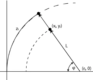
The first tentacle path is defined by boundaries of vertical equations defined by the width of the vehicle plus a buffer width. This path is really a special case of the tentacles based on circular motion paths. The straight path is simplified from (2.22) to vertical linear boundaries. This is shown in equation (2.23), where wvehicle is the width of the vehicle,

and wbuf f er is the width of the buffer spacing. If a depth value, with coordinates (xi, yi),

fails this test, the maximum traversable distance is recorded for future comparison with the control algorithm.

ri = lim

(36)

|xi|> wvehicle+wbuf f er (2.23)

If a data point is within the rectangular region, the maximum traversable distance, zmin,

must be recorded, shown in equation (2.24).

zmin =min(zmin, yi) (2.24)

The main tentacle paths are defined by arc regions. The arc regions have a center radius defined by the potential radii of steering. The definition of the center curve path is defined by Equation (2.33) .

Figure 2.3: A front-wheel-steering vehicle [2]

Calculating the radii of the curve is determined by the following equations [2]: R=

q

a2

2+l2cot2δ (2.25)

cotδ = cotδo+cotδi

2 (2.26)

Rmin =R−

w

2 (2.27)

Rmax =R+ s

R+ w 2

2

+ (l+g)2 _(2.28)

(37)

the front and rear axle. w is the width between the centers of the wheels. δ is the angle from the horizon to the line that goes from the center of the turning radius to the center of the front axle. This distance of the center of mass from the rear axle was experimentally determined to by setting the steering servo to the maximum steering angle, and driven on a carpet surface (tile and concrete surfaces were not enough friction to accurately drive in a circle without slip). The equation was rearranged for a2, shown in equation (2.29).

a2 =

√

R2₋_l2_cot2_δ _(2.29) The value was averaged from 25 trials, and determined to be 20.5 cm.

If a data point is within the arc region, the maximum traversable distance must be calculated (2.30) in reference to the center of the vehicles path and then record the minimum distance (2.32) . The equation (2.31) is based on the law of cosines, calculating the magnitude of the angle from the triangles side lengths.

Figure 2.4: A point inside region, find minimum distance on arc path

L=

q

(|xi| −R)2+yi2 (2.30)

φ=cos−1

R2+L2 −px2

i +y2i

2RL

(2.31)

(38)

The equations (2.34) and (2.35) are the definitions for the outer and inner boundaries of the arcs, respectively. The +- refers to the steering direction (- referring to steering to the right, + for steering to the left)

y=

q

radii2

j −x2 (2.33)

yi > q

(Rmax+wbuf f er)

2

±x2

i (2.34)

yi < q

(Rmin−wbuf f er)

2

±x2

i (2.35)

The veers were created as a way for simplifying the number of CPU intensive math functions. The veers were designed to eliminate the need for large radii curves. The equations (2.36) and (2.37) define the upper an lower bounds of the veer paths. θ is the angle of the veer from the center of the vehicle. Substituting veer paths for large radii curves has been beneficial for low performance hardware, or software platforms where the amount of processing time for path detection needs to be reduced.

yi > xicot(θ) +

w/2 +wbuf f er

cos(θ) (2.36)

yi < xicot(θ)−

w/2 +wbuf f er

(39)

Experimental Setup

3.1 Research Methodology

3.1.1 Software

Analyzing the kernel performance is critical to this research. The tool chosen to perform this for the AMD CPU and the ATI Radeon HD 7970 is AMD’s CodeXL tool. This tool can run as a stand alone application or as an add on to Microsoft Visual Studio. In this research, it is used as an add on to Microsoft Visual Studio 2013. CodeXL is an OpenCL kernel debugger as well as a CPU and GPU profiler tool for running analysis on code. CodeXL is developed by AMD, and is designed to debug OpenCL and OpenGL kernels. The debugger is designed to find any bugs in the kernel code, as well as optimizing performance. The de-bugger is designed to monitor the memory resources, core performance, memory leaks, and areas causing less than optimal kernel execution. The CPU Profiler is designed to analyze the code execution on CPU’s and monitor the resources used during execution. The GPU Profiler collects and visualizes GPU data, kernel occupancy, and hotspot analysis for AMD APUs and GPUs. The Static Kernel Analysis tool allows for kernel code to be compiled for various AMD hardware and simulate the execution time and performance without running the application. This allows for theoretical benchmarking on hardware not in the system. For the Intel CPUs, the Intel OpenCL SDK Debugger was chosen. This debugger does

(40)

not provide as many features as AMD’s CodeXL, Intel’s debugger has been designed and optimized for Intel CPUs. For the NVIDIA GPU, the NVIDIA Nsight debugger add on for Microsoft Visual studio has been chosen as it is designed and optimized to analyze the performance of NVIDIA GPUs in the execution of OpenCL kernels.

The implemented software is grouped into two main test groups: the library functions, implementation using library functions. The library of OpenCL accelerated functions are kernels written that can be executed individually on an OpenCL compatible device, or be used as a reference function from another kernel. The OpenCL enabled library of LiDAR based functions will be individually benchmarked and tested against the C++ implemented code. These functions were discussed in Chapter 2. Since AMD’s CodeXL, Intel’s OpenCL SDK Debugger, and NVIDIA’s Nsight can all profile C++ code, it will be tested with all three profilers. That is, when testing the ATI Radeon HD 7970, CodeXL will profile the C++ implementation as well as the kernel implementation. This will minimize the discrep-ancies in analysis that could come from using three different profilers.

(41)

3.1.2 Hardware

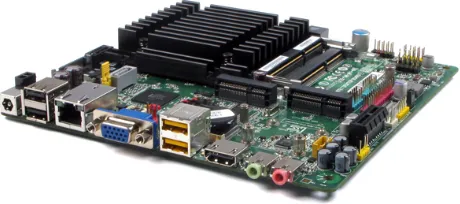
The computer hardware selection was geared to three hardware setups: high wattage system, mobile hardware, and a low power system. The computing hardware for the mobile plat-form consists of an Intel Atom 1.8GHz Mini-ITX motherboard setup, with 4 GB of DDR3 1333MHz RAM. This first test platform requires that the hardware used for implementation must be lightweight, low power. Specifications of this system in Figure 3.1. This setup is a combination of a ultra-low power processor with a low power graphics card. This setup is targeted towards a mobile platform that needs low power and small footprint. This platform is built on the Intel DN2800MT Marshaltown Low Profile Mini ITX Motherboard, shown in ??. This has a vertical profile of 20mm. The other benifit is the flexibility of power input,

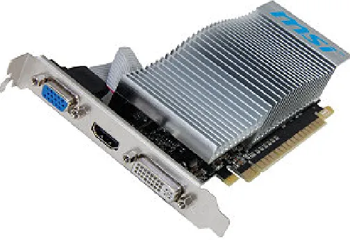
with a power range of 10 to 19V DC. This allows for a lithium polymer batter to be con-nected directly to the motherboard without a DC to DC power converter. The board also features a smart power feature that can automatically shut off if the voltage drops under 11V, protecting batteries from dropping to damagingly low voltages. The MSI GeForce 210 GPU, shown in Figure 3.2, is connected through a PCI Express 1x to 16x ribbon.

Figure 3.1: Intel DN2800MT Marshaltown Low Profile Mini ITX Motherboard

(42)

Figure 3.2: MSI GeForce 210 1GB GDDR3 PCI-Express 2.0

Table 3.3.

CPU 1.8GHz Intel Atom RAM (2) 2GB 1333MHz DDR3 GPU MSI GeForce 210

Table 3.1: Platform 3

CPU 2.6GHz Intel Core i5 RAM (2) 4GB 1866MHz DDR3 GPU NVIDIA 740M

CPU 3.6GHz AMD 6-Core RAM (4) 4GB 1866MHz DDR3 GPU ATI Radeon HD 7970

(43)

in other words a maximum scanning frequency of 10Hz. The detectable range of the sensor is shown in Figure 2.

Figure 3.3: Hokuyo URG-04LX-UG01 LiDAR

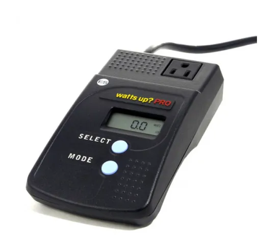
3.1.3 Power Analysis - WattsUp Pro

One of the parameters that is used as a performance metric is the power wattage of of the computer during idle, during CPU load, and during GPU load. This lead to researching various load meters. There are many off-the-shelf load meters available. P3 Kill-A-Watt, Belkin Conserve Insight are popular consumer targeted load meters. Testing began with the P3 Kill-A-Watt. One issue was apparent, while the product boasts an accuracy of 0.2% for wattage, the issue was accurately measuring the wattage. The system does not record data, it only displays data. This limits the accuracy of recording to viewing the device. Any quick power spikes might be missed, and the data cannot be reviewed later.

(44)

Figure 3.4: WattsUp Pro - Power Load Meter

depending on the number of parameters analyzed with each record. Parameters available are Current Watts, Minimum Watts, Maximum Watts, Power Factor, Volt Amp (apparent PWR), Cumulative Watt Hours, Average Monthly KiloWatt Hour, Elapsed Time, Duty Cy-cle, Frequency (Hz), Cumulative Cost, Average Monthly $, Line Voltage, Minimum Volts, Maximum Volts, Current Amps, Minimum Amps, Maximum Amps. The WattsUp Pro is capable of 1Hz power analysis, and has an accuracy of 1.5% for all parameters over 60watts. Under 60 watts, the accuracy of current and power factors is significantly less at approx 10% accuracy. It has a maximum rated power of 1800watts. [insert reference]

(45)

0 200 400 600 800 1,000 1,200 1,400 1,600 0

10 20 30

Time(Seconds)

W

atts

WattsUp Sample Data

To get an accurate power reading for the analysis, the computer hardware will have to be under test load for more than a second.This will reduce the probability that the sampling of the load meter will not accurately take a reading of the test load power, since the test conditions state that the performance metric is to run LiDAR sampling at a rate of 60Hz or faster. In order to accurately test the average power consumed, the software analyzes sample data for 300 readings, which equates to 5 minutes of testing.

An important metric to analyze the power consumed during a non-active state. Background applications have been kept to a minimum and only services needed by the operating system, Windows 8, have been left running. Power will then be measured, and can be compared to the power consumed during data analysis.

3.1.4 Virtual Hardware

(46)

Figure 3.5: Velodyne HDL 64E S2

(47)

Table 3.4: Velodyne HDL 64E S2 - LiDAR Network Protocol

Section Subsection Data Structure Description Header ID 8 byte String ”RDR file”

Options 1 Byte bit0 : 1 if the file contains a lookup table, 0 otherwise bit1-7 : reserved LT Address uint64 Position of the first byte of the

LOOKUP TABLE block in the file if present.

Data Block Timestamp uint64 Milliseconds since the start of the record Packet 27+7*n Bytes A Lidar network protocol packet

(48)

Table 3.5: Velodyne HDL 64E S2 - Data Packet

Section Subsection Data Structure Description

Header Type uint8 Identify the source of the packet [0x01 : real time packet (coming from a live acquisition), 0x02 : sim-ulation packet, 0x03 : replay packet] N uint16 Indicates the number of impacts de-scribed in the IMPACT DATA block. Keep in mind that small packets with a high transmission rate will easily clutter the network. Consider send-ing many impacts in the same pack Sensor Pose X position float West-East axis, east being positive,

in meter

Y position float South-North axis, north being posi-tive, in meter

Z position float Vertical axis, up being positive, in meter

Yaw Angle float In degrees. 0 points to east. 90 points to nort

Pitch Angle float In degrees. 0 points to the horizon. 90 points down

Roll Angle float In degrees. 0 is horizontal. 90 means the left side of the vehicle is pointing up

Impact Data * N Yaw uint16 Between 0 and 35999, the unit is the 100th of degrees. 0 is the for-ward direction. Positive angles go to the left (counter-clockwise when seen from the top of the vehicle)

Pitch uint16 Between 0 and 35999, the unit is the 100th of degree. 0 is the hor-izontal plane in the vehicle’s refer-ence frame. Positive angles go down (counter-clockwise when seen from the left of the vehicle)

Distance uint16 Distance in 0.2 centimeters incre-ments

(49)

Experiment Setup

4.1 OpenCL Accelerated Depth Data Analysis Library

The first step in the analysis of the performance of OpenCL in processing sample LiDAR data was to benchmark the functions written to process the data in terms of :

• Processing time on OpenCL device

• Processing time on CPU without acceleration

• Memory used

• Power Consumed

The algorithms are tested with randomly generated data of various data lengths, as well as sample data from the Hokuyo and the Velodyne HDL 64E S2. The purpose of testing the randomly generated depth data of various lengths is to determine the point at which the efficiency of the processor is greater than using the OpenCL device. For this purpose, data sets of length beginning at 512 to 4294967296 in steps following the equation(4.2), where L is the length of the data set, and i is the step index.

Li = 2i+9 (4.1)

(50)

Testing the kernels with actual data is a necissary step for thorough testing. Sample data from the Hokuyo URG-04LX-UG01 LiDAR will be sampled, and recorded to a data file. The data file will then be used to test each of the kernel functions. Testing will also be done with recorded data provided by Robosoft Inc, France. This data will be from the Velodyne HDL 64E S2 recordings, which were taken from a moving vehicle in an urban environment.

Processing time is analyzed as the time the data is received by the CPU. This is an important benchmark location. For the OpenCL device, at this point all that needs to be done is to initiate the memory transfer from the RAM to the OpenCL device RAM, and then initiate the execution of the kernel. Receiving the data from the depth data device that is used is the same whether a CPU used with the C++ code, or an OpenCL device is used. What needs to be measured though, is the impact that transferring the data to device and the time it takes to execute have in comparison to regular code execution on the CPU. Investigation of the bottleneck in the process is crucial for optimization and measuring the execution time, as well as detailed analysis of how that time is spent is critical to understanding what is happening. AMD CodeXL provides an in depth analysis of the kernel execution and memory transfers, which provides the feedback necessary for this analysis. The end point for the time analysis is when the data has completed transfer off the OpenCL device, and the data is ready for use by the CPU. For consistency of testing the CPU devices, the dynamic clocks on the devices have been disabled. While this does restrict the devices from peak performance, this reduces the discrepancy in time analysis between different tests. These discrepancies arise from how the devices select the operating freqeuncy. The parameters for control are commonly the temperature of the device cores, and power consumption. Something as simple as the environment temperature fluctuating could cause the frequency to be more restricted in one test compared to another.

(51)

Power consumed is an important metric to compare hardware efficiency. As an example, if a performance increases by 40% but the power consumed increases by 80%, the performance gain might not be favorable for the application. To minimize power fluctuations from devices not directly necissary for the experiment, have either been controlled or removed. Heat sink fans of the devices have been controlled to a set fan speed. As well, secondary drives in the system have also been removed to minimize power consumption not related to the experiments.

4.2 Environement Analysis Application of OpenCL

li-brary

The first step in the analysis of the performance of OpenCL in processing sample LiDAR data was to benchmark the functions written to process the data in terms of :

• Processing time on OpenCL device

• Processing time on CPU without acceleration

• Memory used

• Power Consumed

These benchmarks were isolated based on the research of [9] and [11] to be the critical factors when optimizing the execution of the kernel code.

The algorithms are tested with randomly generated data of various data lengths, as well as sample data from the Hokuyo and the Vel. The purpose of testing the randomly generated depth data of various lengths is to determine the point at which the efficiency of the processor is greater than using the OpenCL device. For this purpose, data sets of length beginning at 512 to 4294967296 in steps following the equation(4.2), where L is the length of the data set, and i is the step index.

(52)

Testing the kernels with actual data is a necissary step for thorough testing. Sample data from the Hokuyo URG-04LX-UG01 LiDAR will be sampled, and recorded to a data file. The data file will then be used to test each of the kernel functions. Testing will also be done with recorded data provided by Robosoft Inc, France. This data will be from the Velodyne HDL 64E S2 recordings, which were taken from a moving vehicle in an urban environment.

Processing time is analzed as the time the data is received by the CPU. This is an important benchmark location. For the OpenCL device, at this point all that needs to be done is to initiate the memory transfer from the RAM to the OpenCL device RAM, and then initiate the execution of the kernel. Receiving the data from the depth data device that is used is the same whether a CPU used with the C++ code, or an OpenCL device is used. What needs to be measured though, is the impact that transferring the data to device and the time it takes to execute have in comparison to regular code execution on the CPU. Investigation of the bottleneck in the process is crucial for optimatization and measuring the execution time, as well as detailed analysis of how that time is spent is critical to understanding what is happening. AMD CodeXL provides an in depth analysis of the kernel execution and memory transfers, which provides the feedback necissary for this analysis. The end point for the time analysis is when the data has completed transfer off the OpenCL device, and the data is ready for use by the CPU. For consistency of testing the CPU devices, the dynamic clocks on the devices have been disabled. While this does restrict the devices from peak performance, this reduces the descreptincy in time analysis between different tests. These discreptincies arise from how the devices select the operating freqeuncy. The parameters for control are commonly the temperature of the device cores, and power consumption. Something as simple as the environment temperature fluctuating could cause the frequency to be more restricted in one test compared to another.

(53)

(54)

Chapter 5 Discussion

5.1 Overview

Experiment 1 involves the testing of the execution time of the implementations of the various algorithms on the GPU vs CPU. Using CodeXL, the memory operations and execution time can be analyzed and compared. Using the WattsUp AC Power Analyzer, the power consumed between the CPU and GPU versions can also be analyzed. The cross over point will also be determined. This is the point where the data set size becomes large enough to become more efficient to use the GPU instead of the CPU for the operations.

5.2 Results - Experiment 1

The functions created for this OpenCL accellerated library were tested based on the criteria outlined in Chapter 4. The process for code writing and testing was interated to produce kernel code that was optimized and tested on various hardware platforms. These optimiza-tions include reducing memory operaoptimiza-tions, memory size needed, as well as work group size adjustments. Initial results of kernel performance with little adjustment did show real time performance in most cases (broken down further for each function type), greater performance was gained by changing kernel code to better perform on the OpenCL hardware.

(55)

The hardware platform for final evaluation was the AMD 6 Core CPU with the Radeon 7970 GPU. This platform was selected as the focus hardware, and showed the performance differences between CPU and GPU implentations.

5.2.1 LiDAR Depth Data to 3D Coordinates

Final results of CPU and GPU performance of both C++ implementation, BOOST multi-threading, and OpenCL implementations are shown in the chart 5.2.1 shown below.

−0.1 0 0.1 0.2 0.3 0.4 0.5 0.6 0.7 0.8 0.9 1 1.1

·106 103

104 105 106

Data Set Size

CPU

Cycles

(Tic

ks)

LiDAR Depth Data to 3D Coordinates - Final Results

GPU OpenCL CPU C++ CPU OpenCL

CPU Boost

(56)

Analyzing the memory operations, 72.4% of the total evaluation time was spent on memory transfers from the host to the GPU, and from GPU to host. This is a significant portion of the total operation time, and shows the bottleneck that the system encounters in GPU computing.

The different variations of data types showed similar performance results in terms of com-putation time. The real difference was the memory occupied during operation, which in the cases of the integer variations showed a memory reduction of approximately 24%. This set of functions required very little optimizations from the initial design. The only optimization was changing the number of work items to match the number of possible parallel threads, and dividing the total data set between the work items. The original implementation treated each data point as a work item. This change resulted in a 4% decrease in computation time, which was from a decrease in time spent on queuing.

5.2.2 Data Filtering

−0.1 0 0.1 0.2 0.3 0.4 0.5 0.6 0.7 0.8 0.9 1 1.1

·106 103

104 105 106

Data Set Size

CPU

Cycles

(Tic

ks)

Data Filtering Bandpass - Final Results

CPU Boost

(57)

implementation for the C++, OpenCL, and Boost versions had a maximum power wattage of 220 watts on the AMD system. The GPU version averaged 372 watts on full load. This is a significant increase, 69.1% , of consumed power. There was a performance difference between the OpenCL implementation and the Boost multi threaded versions (in the chart they are overlapping). Both of these were on average 4.5 times performance improvement over the C++ version for OpenCL and Boost library variations. The crossover point for the GPU, this is the point where the GPU outperforms the CPU is 3112 data points. For the large data set, the GPU was 215 times faster.

Analyzing the memory operations, 82% of the total evaluation time was spent on memory transfers from the host to the GPU, and from GPU to host. This is a significant portion of the total operation time, and shows the bottleneck that the system encounters in GPU computing. This bottleneck is increased due to the increased delay in transferring the output to the host. Since the data set might not be smaller than the input due to filter that was removed, the threads now have to push data back asynchronously, and this can cause a performance delay if the memory is being used by another thread.

5.2.3 Global Geometric Translation

−0.1 0 0.1 0.2 0.3 0.4 0.5 0.6 0.7 0.8 0.9 1 1.1

·106 103

104 105 106

Data Set Size

CPU

Cycles

(Tic

ks)

Global Geometric Translation

(58)

As it can be seen, the GPU significantly out performs the CPU implementations of the same calculations. This did however come at a cost of power consumed. During the CPU implementation for the C++, OpenCL, and Boost versions had a maximum power wattage of 220 watts on the AMD system. The GPU version averaged 372 watts on full load. This is a significant increase, 69.1% , of consumed power. There was a performance difference between the OpenCL implementation and the Boost multi threaded versions (in the chart they are overlapping). Both of these were on average 4.5 times performance improvement over the C++ version for OpenCL and Boost library variations. The crossover point for the GPU, this is the point where the GPU outperforms the CPU is 3112 data points. For the large data set, the GPU was 265 times faster. This is a much greater increase in performance of GPU vs CPU, and this comes from the advantage the GPU has for implementing 3D translation and floating point math, being optimized for 3D calculations.

Analyzing the memory operations, 56.9% of the total evaluation time was spent on memory transfers from the host to the GPU, and from GPU to host. This is a significant portion of the total operation time, and shows the bottleneck that the system encounters in GPU computing.

5.2.4 Scale Data

(59)

−0.1 0 0.1 0.2 0.3 0.4 0.5 0.6 0.7 0.8 0.9 1 1.1

·106 103

104 105 106

Data Set Size

CPU

Cycles

(Tic

ks)

Scale Data - Final Results

CPU Boost

As it can be seen, the GPU significantly out performs the CPU implementations of the same calculations. This did however come at a cost of power consumed. During the CPU implementation for the C++, OpenCL, and Boost versions had a maximum power wattage of 220 watts on the AMD system. The GPU version averaged 372 watts on full load. This is a significant increase, 69.1% , of consumed power. There was a performance difference between the OpenCL implementation and the Boost multi threaded versions (in the chart they are overlapping). Both of these were on average 4.5 times performance improvement over the C++ version for OpenCL and Boost library variations. The crossover point for the GPU, this is the point where the GPU outperforms the CPU is 3072 data points. For the large data set, the GPU was 242 times faster. This is a much greater increase in performance of GPU vs CPU, and this comes from the advantage the GPU has for implementing 3D translation and floating point math, being optimized for 3D calculations.

(60)

5.2.5 Gausian Blur

−0.1 0 0.1 0.2 0.3 0.4 0.5 0.6 0.7 0.8 0.9 1 1.1

·106 103

104 105 106

Data Set Size

CPU

Cycles

(Tic

ks)

Gaussian Filter - Final Results

CPU Boost

As it can be seen, the GPU significantly out performs the CPU implementations of the same calculations. This did however come at a cost of power consumed. During the CPU implementation for the C++, OpenCL, and Boost versions had a maximum power wattage of 220 watts on the AMD system. The GPU version averaged 372 watts on full load. This is a significant increase, 69.1% , of consumed power. There was a performance difference between the OpenCL implementation and the Boost multi threaded versions (in the chart they are overlapping). Both of these were on average 4.8 times performance improvement over the C++ version for OpenCL and Boost library variations. The crossover point for the GPU, this is the point where the GPU outperforms the CPU is 3072 data points. For the large data set, the GPU was 205 times faster.

(61)

input data, but depending on the size of the Gaussian filter, up to 8 other data points before and after each work item. This creates a lot of work items that are requesting memory transfers, and creates a memory bottleneck.