Designs of Digital Filters and Neural Networks using Firefly Algorithm

(1)

University of Windsor University of Windsor

Scholarship at UWindsor

Electronic Theses and Dissertations Theses, Dissertations, and Major Papers

2017

Designs of Digital Filters and Neural Networks using Firefly

Algorithm

Ghazanfer Ali University of Windsor

Follow this and additional works at: https://scholar.uwindsor.ca/etd

Recommended Citation Recommended Citation

Ali, Ghazanfer, "Designs of Digital Filters and Neural Networks using Firefly Algorithm" (2017). Electronic Theses and Dissertations. 7344.

https://scholar.uwindsor.ca/etd/7344

This online database contains the full-text of PhD dissertations and Masters’ theses of University of Windsor students from 1954 forward. These documents are made available for personal study and research purposes only, in accordance with the Canadian Copyright Act and the Creative Commons license—CC BY-NC-ND (Attribution, Non-Commercial, No Derivative Works). Under this license, works must always be attributed to the copyright holder (original author), cannot be used for any commercial purposes, and may not be altered. Any other use would require the permission of the copyright holder. Students may inquire about withdrawing their dissertation and/or thesis from this database. For additional inquiries, please contact the repository administrator via email

(2)

Designs of Digital Filters and Neural Networks using Firefly

Algorithm

By

Ghazanfer Ali

A Thesis

Submitted to the Faculty of Graduate Studies

through the Department of Electrical and Computer Engineering in Partial Fulfillment of the Requirements for

the Degree of Master of Applied Science at the University of Windsor

Windsor, Ontario, Canada

2017

(3)

Designs of Digital Filters and Neural Networks using Firefly Algorithm

by

Ghazanfer Ali

APPROVED BY:

______________________________________________ F. Baki

Odette School of Business

______________________________________________ H. Wu

Department of Electrical and Computer Engineering

_____________________________________________ H. K. Kwan, Advisor

Department of Electrical and Computer Engineering

(4)

iii

DECLARATION OF ORIGINALITY

I hereby certify that I am the sole author of this thesis and that no part of this thesis has been published or submitted for publication.

I certify that, to the best of my knowledge, my thesis does not infringe upon anyone’s copyright

nor violate any proprietary rights and that any ideas, techniques, quotations, or any other material from the work of other people included in my thesis, published or otherwise, are fully acknowledged in accordance with the standard referencing practices. Furthermore, to the extent that I have included copyrighted material that surpasses the bounds of fair dealing within the meaning of the Canada Copyright Act, I certify that I have obtained a written permission from the copyright owner(s) to include such material(s) in my thesis and have included copies of such copyright clearances to my appendix.

(5)

iv

ABSTRACT

Firefly algorithm is an evolutionary algorithm that can be used to solve complex multi-parameter problems in less time. The algorithm was applied to design digital filters of different orders as well as to determine the parameters of complex neural network designs. Digital filters have several applications in the fields of control systems, aerospace, telecommunication, medical equipment and applications, digital appliances, audio recognition processes etc. An Artificial Neural Network (ANN) is an information processing paradigm that is inspired by the way biological nervous systems, such as the brain, processes information and can be simulated using a computer to perform certain specific tasks like clustering, classification, and pattern recognition etc. The results of the designs using Firefly algorithm was compared to the state of the art algorithms and found that the digital filter designs produce results close to the Parks McClellan method which shows the algorithm’s capability of handling complex problems.

(6)

v

ACKNOWLEDGEMENTS

(7)

vi

LIST OF TABLES

TABLE 1.1Symmetric Filters ... 8

TABLE 2.1 Comparison of algorithm performance ... 36

TABLE 4.1 2-input one output Neural network design parameters ... 53

TABLE 4.2 2-input one output Neural network design ... 53

TABLE 4.3 Results table with no input noise. ... 57

TABLE 4.4 Results table with 5% input noise. ... 58

TABLE 5.1 Coefficients of 24th-order type1 Lowpass LP-FIR filter by FA ... 61

TABLE 5.2 Coefficients of 24th-order type1 Highpass LP-FIR filter by FA ... 62

TABLE 5.3 Coefficients of 24th-order type1 Bandpass LP-FIR filter by FA... 63

TABLE 5.4 Coefficients of 24th-order type1 Bandstop LP-FIR filter by FA ... 64

TABLE 5.5 24 order FIR type 1 filter design results comparison ... 68

TABLE 5.7 Coefficients of 48th-order type1 Lowpass LP-FIR filter by FA ... 74

TABLE 5.8 Coefficients of 48th-order type1 Highpass LP-FIR filter by FA ... 75

TABLE 5.9 Coefficients of 48th-order type1 Bandstop LP-FIR filter by FA ... 77

TABLE 5.10 Coefficients of 48th-order type1 Bandpass LP-FIR filter by FA... 78

TABLE 5.11 48th order FIR type 1 filter design results comparison ... 81

TABLE 5.13 Coefficients of 24th-order type1 Lowpass LP-GFIR filter by FA ... 86

TABLE 5.14 Coefficients of 24th-order type1 Highpass LP-GFIR filter by FA .. 88

TABLE 5.15 Coefficients of 24th-order type1 Bandpass LP-GFIR filter by FA .. 90

TABLE 5.16 Coefficients of 24th-order type1 Bandstop LP-GFIR filter by FA .. 92

(11)

x

LIST OF FIGURES

Figure 1.1 Digital filter working sequence ... 1

Figure 1.2 Types of filters based on the frequency response ... 3

Figure 1.3 Ideal Lowpass digital FIR filter. ... 5

Figure 1.4 Practical lowpass digital filter ... 6

Figure 1.5 FIR direct form ... 7

Figure 1.6 FIR filter in transposed direct form ... 8

Figure 1.7 Type I FIR filter coefficients ... 10

Figure 1.8 Phase response of a linear phase filter ... 11

Figure 1.9 lowpass digital FIR filter using DE ... 28

Figure 1.10 Bandpass digital FIR filter using DE ... 28

Figure 1.11 Highpass digital FIR filter using DE ... 29

Figure 1.12 Bandstop digital FIR filter using DE ... 29

Figure 4.1 Neural network design for two input XOR problem. ... 52

Figure 4.2 XOR output with 2 input grid ... 54

Figure 4.3 2-dimensional view of Figure 4.2 ... 54

Figure 4.4 Training pattern pairs... 56

Figure 4.5 Ten digit problem output pattern. ... 57

Figure 5.1 24 order Lowpass digital FIR filter using FA... 61

Figure 5.2 24 order Highpass digital FIR filter using FA ... 62

Figure 5.3 24 order Bandpass digital FIR filter using FA ... 63

Figure 5.4 24 order Bandstop digital FIR filter using FA ... 64

Figure 5.5 Lowpass FIR filter comparing FA and DE ... 65

Figure 5.6 Highpass FIR filter comparing FA and DE ... 66

Figure 5.7 Bandpass FIR filter comparing FA and DE... 66

Figure 5.8 Bandstop FIR filter comparing FA and DE ... 67

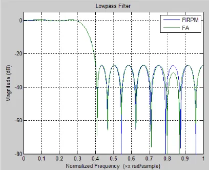
Figure 5.9 Lowpass FIR filter comparing FA and FIRPM ... 69

Figure 5.10 Highpass FIR filter comparing FA and FIRPM ... 70

Figure 5.11 Bandpass FIR filter comparing FA and FIRPM ... 70

Figure 5.12 Bandstop FIR filter comparing FA and FIRPM ... 71

(12)

xi

Figure 5.14 48 order Lowpass digital FIR filter using FA... 73

Figure 5.15 Magnitude response of 48 order Lowpass digital FIR filter ... 74

Figure 5.16 48 order Highpass digital FIR filter using FA ... 75

Figure 5.17 Magnitude response of 48 order Bandstop digital FIR filter ... 76

Figure 5.18 48 order Bandstop digital FIR filter using FA ... 76

Figure 5.19 Magnitude response of 48 order Bandpass digital FIR filter... 77

Figure 5.20 8 order Bandpass digital FIR filter using FA ... 78

Figure 5.21 Lowpass 48 order FIR filter comparing FA and DE ... 79

Figure 5.22 Highpass 48 order FIR filter comparing FA and DE... 79

Figure 5.23 Bandpass 48 order FIR filter comparing FA and DE ... 80

Figure 5.24 Bandstop 48 order FIR filter comparing FA and DE ... 80

Figure 5.25 Lowpass 48 order FIR filter comparing FA and FIRPM... 82

Figure 5.26 Highpass 48 order FIR filter comparing FA and FIRPM ... 82

Figure 5.27 Bandpass 48 order FIR filter comparing FA and FIRPM ... 83

Figure 5.28 Bandstop 48 order FIR filter comparing FA and FIRPM ... 83

Figure 5.29 Lowpass GFIR filter using FA ... 85

Figure 5.30 Passband Group delay of Lowpass GFIR filter using FA ... 86

Figure 5.31 Highpass GFIR filter using FA ... 87

Figure 5.32 Passband Group delay of Highpass GFIR filter using FA... 87

Figure 5.33 Bandpass GFIR filter using FA ... 89

Figure 5.34 Passband Group delay of Bandpass GFIR filter using FA ... 89

Figure 5.35 Bandstop GFIR filter using FA ... 91

(13)

xii

LIST OF ABBREVIATIONS/SYMBOLS

FA PM DE 𝑫(𝝎) 𝜹 𝜹_𝒑 𝜹_𝒔 𝑬(𝝎) FIR g GA 𝒉𝒌 𝑯(𝝎) IIR LP N NP Obj Pmax Pmin Firefly Algorithm Parks-McClellan Method Differential Evolution

Desired frequency response

Passband ripple

Specified passband ripple

Specified stopband ripple

Weighted error function

Finite Impulse Response

Passband gain

Genetic Algorithm

kth filter coefficient

Frequency response of the filter

Infinite Impulse Response

Linear Program

Filter length

Non-deterministic Polynomial Time

Objective function value

Maximum absolute value of frequency response in passband

(14)

xiii PSO

SA

Smax

𝑾(𝝎)

𝝎

𝝎_𝒑

𝝎𝒔

GFIR

Pg

Particle Swarm Optimization

Simulated Annealing

Maximum absolute value of frequency response in stopband

Weighting function

Normalized frequency

Passband cut-off frequency

Stopband cut-off frequency

General Finite Impulse Response

(15)

1

Chapter 1 Introduction

As the technology is reaching its heights, there’s a lot of research work continuing in the

field of digital filters in order to increase their performance, speed and reduce the size, power, and cost of the end products. Digital filters are discrete time devices used to perform operations on an input signal to obtain an output sequence according to a pre-designed difference equation. Inside a digital filter, every sample from input to output sequences with their coefficient values are quantized to a definite word length and are then presented in the form of a binary sequence.

The block diagram representing the working of a digital filter can be seen in fig 1.1.

(16)

2

1.1 Why Digital filters?

Digital filters offer a number of applications with many advantages over analog filters. These advantages of digital filters affect the speed and performances of the overall system as compared to the same system being used with analog filters which require advanced mathematical knowledge and an understanding of the processes involved in the system affecting the filter. Few of the many good characteristics of digital filters as described in Kwan [3] are given below:

 Reliability: Digital filters are reliable that is there is no tolerance problem or aging

in them.

 Accurate: By adjusting the digital word length, one can precisely control the

accuracy of digital filters. It can be made approximately equal or extremely close to the ideal values by adjusting the characteristics of a digital filter.

 Flexible: By having another set of coefficient values, one can easily change the

characteristics of a digital filter.

 Accommodating: It is possible to filter input sequences without any hardware

replication.

 Efficient: Digital filters have a superior performance-to-cost ratio anddo not drift

with temperature or humidity or require precision components.

 Simplicity: Digital filters are software programmable, which makes them easy to

build and test. Digital filters require only the arithmetic operations of addition, subtraction, and multiplication.

(17)

3

1.2 Types of filters

1.2.1 Based on the frequency response

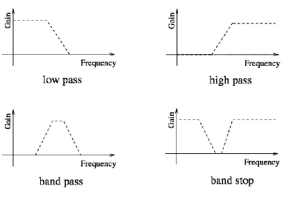
Based on the frequency response, the filters can be categorized in the following 4 common types, as shown in the Fig. 1.1.

Figure 1.2 Types of filters based on the frequency response

These are described below:

1. Low pass filter: The low pass filter allows low frequencies to pass while removing the high frequencies.

2. High pass filter: The high pass filter allows high frequencies to pass while removing the low frequencies.

3. Bandpass filter: The bandpass filter allows only a certain band of frequencies to pass. 4. Bandstop filter: The bandstop filter allows all frequencies to pass except a band which

(18)

4

In addition to these basic types, there are other types such as notch filters, comb filters, etc. The slanted part of the frequency response of the filters is called the transition region, in which the frequency response transitions from the pass band to stop band or vice versa. A good filter must have a narrow transition band.

1.2.2 Based on the impulse response

Based on the impulse response, there are 2 categories of digital filters, namely, finite impulse response (FIR) and infinite impulse response (IIR) filters. As the names suggest, when an impulse input is given to the FIR filter, the output decays to 0 in a finite amount of time. On the other hand, the output takes an infinite amount of time to decay to 0 in the case of an IIR filter. This is due to the recursive nature of an IIR filter, where the output is fed back to the filter, resulting in an output even when the input has been stopped.

1.3 Digital FIR filter design

FIR is short for finite impulse response and is also called non-recursive filter. This kind of digital filter exhibits a finite duration impulse response. An FIR filter is designed by finding the coefficients and filter order that meets certain specifications, which can be in the time-domain (e.g. a matched filter) and/or the frequency time-domain (most common). Matched filters perform a cross-correlation between the input signal and a known pulse-shape. The FIR convolution is a cross-correlation between the input signal and a time-reversed copy of the impulse response. Therefore, the matched filters impulse response is "designed" by sampling the known pulse-shape and using those samples in reverse order as the coefficients of the filter For an FIR filter whose impulse response of length 𝑁=𝑅+1, R being the order, is given by 𝐡=[ℎ0 ℎ1 ℎ2 …ℎ𝑁−1]T_{. The transfer function or the z} transform can be written as equation 1.1.

(19)

5

Where H(𝑧) denotes a polynomial written in ascending powers of 𝑧−1. The coefficients (𝑛) for 𝑛≥0 represent the impulse response values of the FIR digital filter.

When a particular frequency response is desired, several different design methods are common:

 Window design method

 Frequency Sampling method

 Weighted least squares design

 Parks-McClellan method

.

Figure 1.3 Ideal Lowpass digital FIR filter. (Kwan [3], 2016, pg 18)

(20)

6

software simulating, the proper specifications such as amplitude response and phase properties can be completed.

Figure 1.4 Practical lowpass digital filter

(21)

7

Figure 1.5 FIR direct form 1

The output of the filter can be written in the following equation form:

𝑦[𝑘] = ℎ0𝑥[𝑘] + ℎ1𝑥[𝑘 − 1] + ⋯ + ℎ𝑛−1𝑥[𝑘 − 𝑁 + 1] (1.2)

The transfer function of the FIR filter in the 𝑧-domain can be written as

𝐻(𝑧) = ∑ ℎ_𝑛𝑧−𝑛 𝑁−1

𝑛=0

(1.3)

The frequency response of the filter can be found by substituting 𝑧 with 𝑒𝑗𝜔𝑇 as shown below, where 𝜔 is the frequency of the input signal.

𝐻(𝑒𝑗𝜔𝑇 ) = ∑ ℎ𝑛𝑒−𝑗𝜔𝑛𝑇 𝑁−1

𝑛=0

= ∑ ℎ𝑛cos (𝜔𝑛𝑇) 𝑁−1

𝑛=0

− 𝑗 ∑ ℎ𝑛sin (𝜔𝑛𝑇) 𝑁−1

𝑛=0

(22)

8

Generally, in practical implementations, the direct transposed form is used for the FIR filter. This has the advantage, as it does not require the extra shift register for the input.

Figure 1.6 FIR filter in transposed direct form

1.3.1 Linear Phase Filters

The equations 1.2-1.4 represent general FIR filters with the arbitrary magnitude and phase response. It can be shown that it is possible to construct FIR filters with linear phase response. This is possible when the filter coefficients have an even or odd symmetry. Depending on the order of the filter and the symmetry of the filter coefficients, the linear phase filters can be of four types as shown in Table 1.1.

TABLE 1.1 Symmetric Filters

Type Order Symmetry 𝑯(𝝎)at 𝝎 = 𝟎 𝑯(𝝎) at 𝝎 = 𝝅/𝑻

Type I even even any any

Type II odd even any 0

Type III even odd 0 0

(23)

9

If ℎ0,ℎ1… ℎ𝑁−1 are the filter coefficients, where 𝑁 is the length of the filter, then the

following relations hold for the coefficients of the different types of filters.

Type I: ℎ_𝑘 = ℎ_{𝑁−𝑘+1}, 𝑁 is odd

Type II: ℎ_𝑘 = ℎ_{𝑁−𝑘+1}, 𝑁 is even

Type III: ℎ_𝑘 = −ℎ_{𝑁−𝑘+1}, 𝑁 is even

Type IV: ℎ𝑘 = −ℎ𝑁−𝑘+1, 𝑁 is odd

(1.5)

The amplitude responses of the four types of the filters can be expressed by the following equations:

Type I:

𝐻(𝜔) = ℎ(𝑀) + 2 ∑ ℎ𝑛cos ((𝑀 − 𝑛)𝜔) 𝑀−1

𝑛=0

(1.6)

Type II:

𝐻(𝜔) = 2 ∑ ℎ_𝑛cos ((𝑀 − 𝑛)𝜔)

𝑁/2−1

𝑛=0

(1.7)

Type III:

𝐻(𝜔) = 2 ∑ ℎ_𝑛sin ((𝑀 − 𝑛)𝜔)

𝑀−1

𝑛=0

(24)

10 Type IV:

𝐻(𝜔) = 2 ∑ ℎ𝑛cos ((𝑀 − 𝑛)𝜔) 𝑁/2−1

𝑛=0

(1.9)

Where 𝑀 = (𝑁 − 1)/2

It can be seen that Type I can be used to construct both low and high pass filters, Type II can be used to construct only low pass filters, Type IV can be used to construct only high pass filters and Type III can be used to construct only bandpass filters. Due to this, Type I filters are most common.

In the following figure, coefficient values of a Type I linear phase filter are shown:

(25)

11

The coefficients are symmetric around the central coefficient, as can be seen in the above figure. The phase response of a linear phase filter is shown in the following figure

Figure 1.8 Phase response of a linear phase filter

We can see that the phase response of the filter varies linearly. The discontinuities are due to two reasons:

(26)

12

1.4 Design of FIR filters

FIR filters can be designed using various methods. The most common of these methods are:

1. Equi-ripple (minimax) design in which the maximum frequency response error from the specified frequency response is minimized. Parks-McClellan method can be used to design FIR filters based on minimax criterion.

2. Least mean square design, in which the mean square error is minimized from the desired frequency response.

3. Window-based methods based on inverse DFT.

Here, we will focus on the minimax design of FIR filters, as this is the criterion on which the work in this thesis is based.

1.4.1 Equi-ripple design of linear phase FIR filters

The transfer function of the Type 1 filter is shown in equation (2.1) as

H(𝐜, w) = e−j(M−12 )wT{h (M−1

2 ) + ∑ 2h(n) M−3

2

n=0 cos [( M−1

2 − n) wT]} (1.10)

H(𝐜, w) = e−j(M−12 )wTA(𝐜, w)_(1.11)

Where,

A(𝐜, w) = 𝐜T𝐜𝐨𝐬 (w) (1.12)

And,

𝐜𝐨𝐬(w) = [1 cos(wT) cos(2wT) ⋯ cos (M−1

2 wT)]

T

(27)

13

The coefficient vector 𝐜T_{is optimized initially starting with the random values and then}

following the structure of the algorithm used to reduce the objective function value at every iteration which I reduced by minimizing the error value at every iteration. To calculate the error, the minimax error approximation method is used. It takes the error between the frequency response of the ideal and designed filter. An ideal filter has a magnitude of 1 on the passband and 0 on the stopbands. So, the error of the iteration values is given by the absolute difference between the ideal magnitudes and the actual filter coefficient values in that iteration. The expression of the minimax function is given by

e_p(𝐜) = [∑Ip_i=1W_p(w_i)||A(𝐜, w_i)| − A_d(w_i)|2p]1/2p

for W_p(w_i) ≥ 0; 0 ≤ w_i ≤ w_p (1.14)

es(𝐜) = [∑ Ws(wi)||A(𝐜, wi)| − Ad(wi)| 2p Is

i=1 ]

1/2p

for Ws(wi) ≥ 0; ws ≤ wi ≤ π

(1.15)

Where e_p(𝐜) and e_s(𝐜) are the error values in the passband and stopband respectively.

A(𝐜, w_i) is the magnitude response of the ideal filter and A_d(w_i) is the magnitude response of the desired filter. and i is the number of samples used to calculate the error. The minimax optimization problem is to search for an optimal coefficient vector 𝐜 that minimizes the objective function e(𝐜) as

min

𝐜 e(𝐜) (1.16)

W_s(w_i) represents the weighting function which is given by:

(28)

14

Weighting scores may vary depending on the error values and if the error of passband and stopband values differs by quite a margin then the weight values can be increased or decreased accordingly.

Figure 1.3 represents the desired filter response, which corresponds to an ideal low-pass filter, with cut-off frequency 𝜔_𝑐. The response is exactly 1 in the passband and drops to 0 in the stopband sharply. In practical filters of finite length, the frequency response deviates from the ideal response as shown in the solid curve in the figure 1.4. Therefore, the specifications of practical filters are relaxed compared to the ideal filters.

The interval 0-𝜔_𝑝 is the pass-band and 𝜔_𝑐-1 is the stop-band of the filter. For the designed filter, in the pass-band, the response can vary from 1-𝛿𝑝 to 1+𝛿𝑝 and in the stopband from

-𝛿_𝑠 to 𝛿_𝑠. In the transition region, which is from 𝜔_𝑝 to 𝜔_𝑠 the response can take any value.

𝛿_𝑝 is called the pass-band ripple and 𝛿_𝑠 the stop-band ripple. The tighter the filter specifications are, the higher the filter length, 𝑁 is required to design the filter.

The above design problem can be formulated as a linear program shown in the following equations:

Minimize 𝜹

Such that: 1 − 𝛿 ≤ 𝐻(𝜔) ≤ 1 + 𝛿, for 𝜔 ∈ [0, 𝜔_𝑝]

−(𝛿_𝑠𝛿)/𝛿_𝑝≤ 𝐻(𝜔) ≤ (𝛿_𝑠𝛿)/𝛿_𝑝, for 𝜔 ∈ [ 𝜔_𝑠, 1] (1.17)

Where, 𝐻(𝜔) is the frequency response of the filter and is given by

𝐻(𝜔) = ∑ ℎ(𝑛)Trig(𝜔, 𝑛)

⌊𝑁−1₂ ⌋

𝑛=0

(29)

15

Where N is the filter length and Trig is a trigonometric function depending on the type of the filter and whether the filter length is odd or even (See equations 1.6-1.9).

Solving the linear program (LP), we can find the values ofthe filter coefficients ℎ(𝑛) and the ripple 𝛿.

The filter can be instead designed using Parks-McClellan method which is very efficient. This is an iterative algorithm, reducing the maximum error in each iteration. The MATLAB function firpm is based on the Parks-McClellan method and can be used to design linear-phase FIR filters with a given length and specified pass and stop bands. The syntax of the function is shown below:

b = firpm(n,f,a,w)

where, n is the filter order, which is one less than the filter length,

f and a define the pass and stop bands. For example, f = [0 0.3 0.5 1], and a = [1 1 0 0] represents a low pass filter with passband from 0 to 0.3𝜋 and stop band from 0.5𝜋 to 𝜋.

w is the weight vector of length equal to the number of bands. Each value in the vector represents the weight assigned to the corresponding band of the filter.

1.4.2 Advantages of FIR filters

An FIR filter has a number of useful properties which sometimes make it preferable to an infinite impulse response (IIR) filter. FIR filters:

 Require no feedback. This means that any rounding errors are not compounded by

summed iterations. The same relative error occurs in each calculation. This also makes implementation simpler.

(30)

16

 Can easily be designed to be linear phase by making the coefficient sequence

symmetric. This property is sometimes desired for phase-sensitive applications, for example, data communications, seismology, crossover filters, and mastering.

The main disadvantage of FIR filters is that considerably more computation power in a general purpose processor is required compared to an IIR filter with similar sharpness or selectivity, especially when low frequency (relative to the sample rate) cut offs are needed. However many digital signal processors provide specialized hardware features to make FIR filters approximately as efficient as IIR for many applications.

1.5 Quantization of coefficients

The continuous filter coefficients can be quantized using either uniform quantization or non-uniform quantization. The uniform quantization can be achieved by the following number representations:

1.5.1 Signed magnitude representation

In this representation, the magnitude of the number is represented by the bits excluding the MSB and the sign of the number is represented by the MSB.

For example: (0101)2 = +510 and (1010)2 = -210

The number 0 has 2 possible representations in this system, which are (0000)2 and (1000)2.

1.5.2 One’s complement representation

In this representation, the negative of a number is equal to bitwise OR of the number.

For example: (0110111)2 = +5510 and (1001000)2 = -5510

In order to add two one’s complement numbers, it is necessary to add the end-around carry

(31)

17 (1110001)2 + (0010000)2 = (1 0000001)2

To obtain the correct answer the carry bit is added to the remaining number, which gives

(1)2 + (0000001)2 = (0000010)2

1.5.3 Two’s complement representation

To avoid the task of adding the carry bit after the addition of two one’s complement numbers, in the two’s complement representation the negative of a number is formed by

taking bit-wise not of the number and then adding 1 to the result.

For example: -5510 is represented by (1001000)2 + (1)2 = (1001001)2

The addition of two 2’s complement numbers is straightforward and can be done using

normal addition.

1.5.4 Signed digit format

In signed digit format each digit of the number has a sign associated with it. One example is balanced ternary, whose base is 3 and the digits can take the values from {-1, 0, 1}.

For example: (1 0 -1 -1)2 = 23 - 21 -20 = 8 – 2 – 1 = 5

The signed digit format is not unique.

1.5.5 Canonical signed digit representation

If in the signed digit representation no two consecutive digits are non-zero, then the resulting representation is called canonical signed digit representation (CSD). The CSD representation of a number is unique.

1.5.6 Non-uniform quantization

(32)

18

coefficients. Limiting the number to 2, the filter coefficients are then represented by the following equation

ℎ𝑛 = 𝑐𝑛12−𝑏𝑛1+ 𝑐𝑛22−𝑏𝑛2 (1.19)

Where,

𝑐_𝑛1, 𝑐_𝑛2∈ {−1,0,1} and 𝑏_𝑛1, 𝑏_𝑛2∈ {1,2, … 𝑏}

1.5.7 Integer representation of coefficients

The coefficients are quantized to a certain number of bits in an algorithm. The number of digits in binary format of a coefficient, proceeding initial zeros after quantization is called the effective word-length of the coefficient. For example, consider a filter with 3 coefficients with values 0.4569, -0.2438 and 0.1211. The binary values of these coefficients are

0.01110100111101110110…, -0.00111110011010011010… and 0.00011111000000000110…

If these are rounded to 9 digits after the binary point, then the values become

0.011101010, -0.001111101 and 0.000111110

The EWL of each coefficient is then equal to the number of digits of each coefficient after the initial zeros, which is 8, 7 and 6 respectively.

Instead of working on these values which are binary, these can be multiplied by a number which is a power of 2, i.e. 2n, such that the resulting values become integers. In the above example, it can be easily seen that this number is 29. Multiplying the coefficients by 29, we get

(33)

19

1.6 Initial Coefficients

The FIR filters and neural network designs selected for optimization has the Initial

coefficients set such that it maximizes the randomization so that all the filter designs can be started from the scratch giving algorithm most of the work which ensures the quality of the design. The initial coefficients used for the designs in this thesis are given as follows:

Let 𝐶_𝑘[𝑈]and 𝐶_𝑘[𝐿]denote the upper bound and the lower bound of the 𝑘th coefficient 𝐶_𝑘 of a LP or HP or BP or BS used in the equations such that

𝐶_𝑘[𝐿] ≤ 𝐶_𝑘 ≤ 𝐶_𝑘[𝑈] 𝑓𝑜𝑟 1 ≤ 𝑘 ≤𝑁

2 + 1 (1.20)

The initial coefficient value of 𝐶_𝑝𝑘 for a population member p is computed by

𝐶_𝑝𝑘 = 𝐶_𝑘[𝐿]+ 𝑟𝑎𝑛𝑑 ∗ (𝐶_𝑘[𝑈]− 𝐶_𝑘[𝐿]) 𝑓𝑜𝑟 𝑝 = 1: 𝑃, 𝑘 = 1: 𝐾 (1.21)

Where 𝑟𝑎𝑛𝑑 is a uniformly distributed value between [0, 1].

1.7 General FIR Filters

(34)

20

manner as the FIR filters given by the equations 1.14 and 1.15. The transfer function of an N-th order FIR digital filter consisting of N+1 coefficients can be written as

𝐻(𝑧) = ∑ 𝑐(𝑛)𝑧−𝑛_{= 𝒄}𝑇_𝒛 𝑁

𝑛=0

(𝑧) (1.22)

From (1.20), it can be seen that c is the coefficient vector and H(z) denotes a polynomial written in ascending powers of 𝑧−1. The magnitude response |𝐻(𝑤)| of GFIR filter is equal to

|𝐻(𝑤)| = {[∑ 𝑐_𝑛cosnwT

𝑁

𝑛=0

]

2

+ [∑ 𝑐_𝑛sinnwT

𝑁 𝑛=0 ] 2 } 1 2 ⁄ (1.23)

The phase response, 𝜃(𝑤) is given by,

𝜃(𝑤) = −𝑡𝑎𝑛−1[∑ 𝑐𝑛sinnwT

𝑁 𝑛=0

∑𝑁 𝑐_𝑛cosnwT

𝑛=0

] (1.24)

From (1.22), the group delay 𝜏(𝑤) can be expressed as

𝜏(𝑤) = −𝜕𝜃(𝑤) 𝜕𝑤𝑇 =

1 1 + 𝑐2

𝜕𝑐

𝜕𝑤𝑇 (1.25)

where

𝑐 = ∑ 𝑐𝑛sinnwT

𝑁 𝑛=0

∑𝑁_𝑛=0𝑐_𝑛cosnwT (1.26)

Taking partial derivative of (1.24), we have

𝜕𝑐 𝜕𝑤𝑇=

[∑𝑁𝑛=0𝑐𝑛cosnwT][∑𝑁𝑛=0𝑛𝑐𝑛cosnwT]

[∑𝑁_𝑛=0𝑐_𝑛cosnwT]2

+ [∑ 𝑐𝑛sinnwT

𝑁

𝑛=0 ][∑𝑁𝑛=0𝑛𝑐𝑛sinnwT]

[∑𝑁𝑛=0𝑐𝑛cosnwT]2

(35)

21

1.8 Optimization algorithms

A number of optimization algorithms have been discussed in [3] which integrates important FIR filter designs with optimization algorithms. In the following section, some important deterministic and heuristic algorithms from the literature are reviewed.

1.8.1 Deterministic algorithms

In computer science, a deterministic algorithm is an algorithm which, given a particular input, will always produce the same output, with the underlying machine always passing through the same sequence of states. Deterministic algorithms are by far the most studied and familiar kind of algorithm, as well as one of the most practical since they can be run on real machines efficiently.

Formally, a deterministic algorithm computes a mathematical function; a function has a unique value for any input in its domain, and the algorithm is a process that produces this particular value as output. If the system is deterministic, this means that from this point onwards, its current state determines what its next state will be; its course through the set of states is predetermined. Note that a system can be deterministic and still never stop or finish, and therefore fail to deliver a result.

If the feasible range of any coefficient is found to be empty at any stage, the algorithm backtracks to the previous quantized coefficient and quantizes it to the next nearest quantization value from the center of its feasible range.

First, the lower and upper bound of each coefficient is calculated [5]. This is done by solving the following linear program problem:

minimize: 𝑓 = ℎ(𝑘) and 𝑓 = −ℎ(𝑘)

such that: 𝑏 − 𝛿 ≤ 𝐻(𝜔) ≤ 𝑏 + 𝛿, for 𝜔 ∈ [0, 𝜔𝑝]

− (𝛿𝑠𝛿) 𝛿⁄ 𝑝≤ 𝐻(𝜔) ≤ (𝛿𝑠𝛿) 𝛿⁄ 𝑝, for 𝜔 ∈ [𝜔𝑠,𝜋]

𝑏𝑙 ≤ 𝑏 ≤ 𝑏ℎ

(36)

22

Where 𝑏 is the passband gain and 𝛿_𝑝 and 𝛿_𝑠 are the maximum allowed pass and stop-band ripple. 𝐻(𝜔) is the magnitude of the frequency response of the filter.

After this, a depth-first search is done and filter coefficients are fixed to integers one by one. Once a coefficient is fixed the remaining un-quantized one are re-optimized.

These algorithms are guaranteed to return an optimum set of filter coefficients, but for filters with high word-lengths, the algorithm takes very long time to finish the search and becomes impractical. The run-time increases exponentially with the increase of the filter length.

A variety of factors can cause an algorithm to behave in a way which is not deterministic, or non-deterministic:

 If it uses external state other than the input, such as user input, a global variable, a

hardware timer value, a random value, or stored disk data.

 If it operates in a way that is timing-sensitive, for example, if it has multiple

processors writing to the same data at the same time. In this case, the precise order in which each processor writes its data will affect the result.

 If a hardware error causes its state to change in an unexpected way.

Although real programs are rarely purely deterministic, it is easier for humans as well as other programs to reason about programs that are. For this reason, most programming languages and especially functional programming languages make an effort to prevent the above events from happening except under controlled conditions.

(37)

23

1.8.2 Heuristic algorithms

The term heuristicis used for algorithms [11] which find solutions among all possible ones, but they do not guarantee that the best will be found, therefore they may be considered as approximately and not accurate algorithms. These algorithms, usually find a solution close to the best one and they find it fast and easily. Sometimes these algorithms can be accurate, that is they actually find the best solution, but the algorithm is still called heuristic until this best solution is proven to be the best. The method used from a heuristic algorithm is one of the known methods, such as greediness, but in order to be easy and fast the algorithm ignores or even suppresses some of the problem's demands.

In [5], GA is used to design FIR filter with coefficients which are constrained to the sums of two numbers, which are powers of two. In order to constrain the search space, a specific coefficient coding scheme is used. Instead of coding the values of the coefficients directly, the differences from some leading values are chosen and coded. The leading values are chosen as the coefficients obtained after quantizing the optimal continuous coefficients. In the case, when the sum of the power of two terms is used, the quantization is done such that the quantized value is the nearest value in the domain. As the optimal discrete filter coefficients are generally relatively not far away from the continuous filter coefficients, therefore the differences to be encoded are not very large and can be encoded using lesser number of bits, compared to encoding the full coefficient values.

Usually, heuristic algorithms are used for problems that cannot be easily solved [34]. Classes of time complexity are deﬁned to distinguish problems according to their “hardness”. Class P consists of all those problems that can be solved on a deterministic

(38)

24

be understood as the class of problems that are NP-complete or harder. NP-hard problems have the same trait as NP-complete problems but they do not necessarily belong to class NP, that is class NP-hard includes also problems for which no algorithms at all can be provided. In order to justify application of some heuristic algorithm, we prove that the problem belongs to the classes NP-complete or NP-hard. Most likely there are no polynomial algorithms to solve such problems, therefore, for suﬃciently great inputs heuristics are developed. Some of the very effective heuristic algorithms are described below:

Swarm intelligence was introduced in 1989. It is an artiﬁcial intelligence technique, based

on the study of collective behavior in decentralized, Self-organized, systems [15, 23, 49]. Two of the most successful types of this approach are Ant Colony Optimization (ACO) and Particle Swarm Optimization (PSO) [3]. In ACO artiﬁcial ants build solutions by moving

on the problem graph and changing it in such a way that future ants can build better solutions. PSO deals with problems in which the best solution can be represented as a point or surface in an n-dimensional space. The main advantage of swarm intelligence techniques is that they are impressively resistant to the local optima problem.

1.8.3 Evolutionary algorithms

Evolutionary algorithms [10, 54] are methods that exploit ideas of biological evolution, such as reproduction, mutation, and recombination, for searching the solution of an optimization problem. They apply the principle of survival on a set of potential solutions to produce gradual approximations to the optimum. A newest of approximations is created by the process of selecting individuals according to their objective function, which is called ﬁtness for evolutionary algorithms and breeding them together using operators inspired

from genetic processes [47]. This process leads to the evolution of populations of individuals that are better suited to their environment than their ancestors. The main loop of evolutionary algorithms includes the following steps:

1. Initialize and evaluate the initial population.

(39)

25 3. Apply genetic operators to generate new solutions.

4. Evaluate solutions in the population.

5. Start again from point 2 and repeat until some convergence criteria are satisﬁed.

Sharing the common idea, evolutionary techniques can diﬀer in the details of

implementation and the problems to which they are applied. Genetic programming searches for solutions in the form of computer programs. Their ﬁtness is determined by the ability to solve a computational problem. The only difference from evolutionary programming is that the latter ﬁxes the structure of the program and allows their numerical

parameters to evolve. Evolution strategy works with vectors of real numbers as representations of solutions and uses self-adaptive mutation rates. The most successful among evolutionary algorithms are Genetic Algorithms (GAs) [5]. They have been investigated by John Holland in 1975 and demonstrate essential eﬀectiveness. GAs are

based on the fact that the role of mutation improves the individual quite seldom and, therefore, they rely mostly on applying recombination operators. They seek solutions to the problems in the form of strings of numbers, usually binary. There are a number of different Evolutionary algorithms that are being developed and are consistently being research on because of their efficiency and effectiveness to perform a complex task in a lesser amount of time. The evolutionary algorithm chosen for this particular thesis is Firefly Algorithm [1] which demonstrates the optimization of complex problems using the

behavior of fireflies. Another algorithm which is further explained in 1.9 is the Differential Evolution (DE) algorithm [6] which is one of the simplest yet effective evolutionary

(40)

26

1.9 Differential Evolution:

In the initial research for this thesis, Differential Evolution method was applied in order to optimize the filter coefficients and obtain error values as minimum as possible. Differential Evolution (DE) [65] is a stochastic parallel search method that can efficiently optimize non-differentiable, nonlinear objective functions. DE requires only a few parameters to manage its operations. The reason why DE is called a parallel method is that it tries to optimize a number of parameter vectors at the same time, thus creating a higher chance of finding a global optimum.

DE creates new members in the solution space by adding and scaling members from the existing population. This makes it a self-referential method. Since scaling and addition are linear operators, the initial probability distribution of the members is kept the same. This property makes the DE scheme completely self-organizing.

The major characteristics of DE include robust; fast, simple and easy to use, effective with good global optimization abilities; inherently parallel; no predefined probability distribution is required; amendable to real, integer and mixed-parameter optimization; precision limited only by floating-point format; and applicable to noisy objective functions.

Differential evolution [65] requires only a few parameters to manage its operations. Using differential evolution does not require knowledge of its underlining principles and other evolutionary optimization techniques. In general, differential evolution is robust; fast; simple and easy to use.

(41)

27

The main steps of the DE algorithm are given below:  𝐼𝑛𝑖𝑡𝑖𝑎𝑙𝑖𝑧𝑎𝑡𝑖𝑜𝑛

 𝐸𝑣𝑎𝑙𝑢𝑎𝑡𝑖𝑜𝑛  𝑚𝑢𝑡𝑎𝑡𝑖𝑜𝑛  𝑐𝑟𝑜𝑠𝑠𝑜𝑣𝑒𝑟

 selection

The crossover probability 𝐶𝑅 controls the fraction of the parameter values that are copied from the mutant. Mutation is applied in this way to each member of the population. If an element of the trial vector is found to violate the bounds after mutation and crossover, it is reset in such a way that the bounds are respected (with the specific protocol depending on the implementation). Then, the objective function values associated with the children are determined.

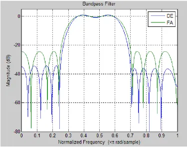
1.9.1 Digital Filters Using DE:

(42)

28

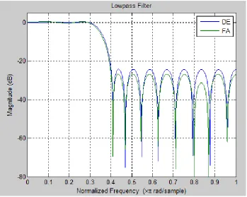
Figure 1.9 lowpass digital FIR filter using DE

(43)

29

Figure 1.11 Highpass digital FIR filter using DE

(44)

30

1.10 Motivation and goals

(45)

31

1.11 Thesis organization

This thesis compromises of a detailed study on Firefly Algorithm and its advantages, It has been used to design digital filters and neural networks and the organization of the compiled data is given as follows:

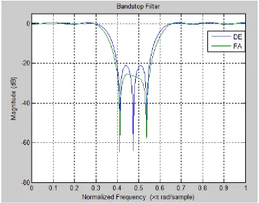
The first chapter has the introduction to the filters, advantages, and disadvantages of using digital filters to state a point why this design has been chosen to be implemented using FA. The conventional methods of filter designing and the common techniques used to design some of the filters. It also contains the motivation and goals of this thesis. The algorithms used in the designing of various filters including deterministic and heuristic methods are also discussed and explained briefly. In addition, a couple of algorithms such as Genetic algorithm and Differential evolution algorithms are also explained which are also used in the later chapters to design the same filters for comparison purposes with FA. In addition, some of the filter designs using DE are also given in the chapter.

In the second chapter, some of the state-of-the-art methods for designing linear phase FIR filters are discussed and the literature is reviewed. In the third chapter, Firefly algorithm is discussed in detail. Its orientation, similarities, advantages, disadvantages and all the information regarding the algorithm is discussed. Its applications before filter designs are also discussed briefly. Also, the mechanism and flow of algorithm are discussed along with its advantages and strong points over other well-known algorithms.

In the fourth chapter, Neural networks are discussed briefly, the need for implementation of neural nets along with its types and applications are discussed. A few described neural network problems are also presented in the chapter with their results using FA.

In the fifth chapter, the results of Firefly algorithm for digital filters and neural networks are analyzed. Some benchmark filters are designed using the algorithm and their frequency responses are presented. The run-time of the algorithm is also calculated and discussed and a comparison is made with the state of the art methods and other algorithms.

(46)

32

The main contribution of the work done here is the implementation of Firefly algorithm and adapting it to make it suitable for designing FIR filters and neural network designs. The algorithm has not been previously used for the design of digital FIR filters. The disadvantage of other algorithms such as GA and PSO is that they require fine-tuning of the parameters. Also, there is a problem of early convergence to a local minimum. FA, on the other hand, is very flexible with parameters, which are relatively easier to tune. Also, it is easy to tune FA such that it doesn’t get trapped in local minima while being a very

(47)

33

Chapter 2 Review of Literature

Filter optimization is not a topic new to us. There have been many advancements in this particular field and a lot of research work has been carried out. But more and more work is being done on daily basis to improve its performance, speed, adaptability and overall efficiency of the system [3]. As discussed in chapter 1, digital filters are an essential part and perhaps one of the most important features of the modern day circuit designs so its accuracy plays a vital role in the improvement of the overall system producing better results.

There have been many methods used for the optimization purposes but one of the most efficient ones have been accomplished using an optimization algorithm [3, 4]. Optimization algorithms are easier to execute, cost-effective and can give you results near to real ones. The improvement of the digital filter is hence dependent on a good performing optimization algorithm [6]. There are a number of high performing optimization algorithms that can be classified into different types with each having a certain advantage over the other. The main focus of this thesis is on Firefly optimization algorithm [1, 9] later explained in Chapter 3 which is a nature-inspired, meta-heuristic algorithm and can solve complex mathematical problems with close to ideal results depending on the parameter values set rightly according to the given problem.

(48)

34

famous problem using firefly algorithm which helps to optimize to the optimal results converging in an acceptable time, which for this test system was approximately 3 seconds.

Xin-She Yang used different complex test functions for FA in [12] to prove the efficiency and optimization capabilities of the algorithm. For the standard pressure vessel design optimization, the optimal solution found by FA is far better than the best solution obtained previously in the literature. In addition, a few new test functions with either singularity or stochastic components were also introduced but with known global optimality, and thus they can be used to validate new optimization algorithms. The optimization results imply that the Firefly Algorithm is potentially more powerful than other existing algorithms such as particle swarm optimization such as those described in [13].X.S.Yang described Firefly algorithm along with other nature-inspired algorithm in [14]. He described the behavior of fireflies, working on the algorithm, its implementation and different modifications to the algorithms [1, 2].

X.Yang in [15] highlighted the importance of exploitation and exploration and their effect on the efficiency of an algorithm. It used the intermittent search strategy theory as a preliminary basis for analyzing these key components and ways to find the possibly optimal settings for algorithm-dependent parameters. It used the firefly algorithm to find this optimal balance and confirmed that firefly algorithm can indeed provide a good balance of exploitation and exploration. It also shows that firefly algorithm requires far fewer function evaluations.

Firefly algorithm has attracted much attention since its development and has been applied to many applications [20, 23, 27, 30, 37, 28,29]. Horng et al. demonstrated that Firefly-based algorithm used least computation time for digital image compression [28, 29], while Banati and Bajaj used firefly algorithm for feature selection and showed that firefly algorithm produced consistent and better performance in terms of time and optimality than other algorithms [21].

(49)

35

optimization and showed that FA can outperform artificial bee colony (ABC) algorithm [23]. In addition, Zaman and Matin have also found that FA can outperform PSO and obtained global best results [41]. Sayadi et al. developed a discrete version of FA which can efficiently solve NP-hard scheduling problems [34], while a detailed analysis has demonstrated the efficiency of FA over a wide range of test problems, including multi-objective load dispatch problems [20, 36, 39]. Furthermore, FA can also solve scheduling and traveling salesman problem in a promising way [28, 30, 40].

Classifications and clustering are another important areas of applications of FA with excellent performance [25, 33]. For example, Senthilnath provided an extensive performance study by compared FA with 11 different algorithms and concluded that firefly algorithm can be efficiently used for clustering [35]. In most cases, firefly algorithm outperforms all other 11 algorithms. In addition, firefly algorithm has also been applied to train neural networks [31]. For optimization in dynamic environments, FA can also be very efficient as shown by Farahani et al. [24, 25] and Abshouri [18].

(50)

36

Various studies show that PSO algorithms can outperform genetic algorithms (GA) and other conventional algorithms for solving many optimization problems. This is partially due to that fact that the broadcasting ability of the current best estimates gives better and quicker convergence towards the optimality. A comparison of the Firefly Algorithms with PSO and genetic algorithms for various standard test functions have been shown in [9]. After implementing these algorithms using MATLAB, extensive simulations have been carried out and each algorithm has been run at least 100 times so as to carry out meaningful statistical analysis. The algorithms stop when the variations of function values are less than a given tolerance ≤ 10−5

. The results are summarized in the following table (see Table 2.1) where the global optima are reached. The numbers are in the format: an average number of evaluations (success rate), so 3752 ± 725(99%) means that the average number (mean) of function evaluations is 3752 with a standard deviation of 725. The success rate of finding the global optima for this algorithm is 99%. We can see that the FA is much more efficient in finding the global optima with higher success rates.

TABLE 2.1 Comparison of algorithm performance for different standard Functions

Functions/Algorithms GA PSO FA

Michalewicz’s (d=16)

Rosenbrock’s (d=16)

De Jong’s (d=256)

Schwefel’s (d=128)

Ackley’s (d=128)

Rastrigin’s

Easom’s

Griewank’s

Shubert’s (18 minima)

Yang’s (d = 16)

89325 ± 7914(95%)

55723 ± 8901(90%)

25412 ± 1237(100%)

227329 ± 7572(95%)

32720 ± 3327(90%)

110523 ± 5199(77%)

19239 ± 3307(92%)

70925 ± 7652(90%)

54077 ± 4997(89%)

27923 ± 3025(83%)

6922 ± 537(98%)

32756 ± 5325(98%)

17040 ± 1123(100%)

14522 ± 1275(97%)

23407 ± 4325(92%)

79491 ± 3715(90%)

17273 ± 2929(90%)

55970 ± 4223(92%)

23992 ± 3755(92%)

14116 ± 2949(90%)

3752 ± 725(99%)

7792 ± 2923(99%)

7217 ± 730(100%)

9902 ± 592(100%)

5293 ± 4920(100%)

15573 ± 4399(100%)

7925 ± 1799(100%)

12592 ± 3715(100%)

12577 ± 2356(100%)

(51)

37

Chapter 3 Firefly Algorithm

3.1 Mathematical model of Firefly algorithm:

Firefly algorithm is organized in a way that it requires the following steps to be set up properly. Not all of these steps are a necessary requirement but helps in implementing the algorithm more efficiently.

1. Set initial parameters in the parameter vector [n iterations α β γ]. Set Upper bound and Lower bound values. (For Example: For a FIR-1 filter, initial values may be set as N=35, iterations=1500, α = 0.25, β = 0.2 and γ=1, Ub=1.5, Lb= -1.5)

2. Generate an initial coefficient vector (say u0). Set the number of coefficients (d) to be optimized.

u0 = Lb + (Ub − Lb) ∗ rand(1, d)

where d =n

2+ 1 for FIR type 1 filter (n=24)

3. Inside the algorithm, calculate the number of evaluations and set up a population matrix P with its size equal to

[number of fireflies, number of filter coefficients to be optimized]

with random values generated around initial coefficient vector u0.

Number of Evaluations = N ∗ iterations

(52)

38

4. From the population matrix obtained, obtain a fitness value for every coefficient vector. There will be (N x 1) number of fitness values obtained. Sort the fitness values of that vector in the ascending order and store the output in an X matrix.

fi = cost(Pi)

X = sort (fi)

5. Obtain fbest value from the X vector (which will always be the topmost value after sorting). Compare every value of X with itself (comparing Xi and Xj,). Calculate the distance ‘rij’ for each of the two compared value.

fbest = XN,1

6. Change every coefficient vector from the population P that satisfies Xi > Xj using

Pi = Pi+ β(Pj – Pi) + α ∗ [rand(1, d) − 1

2] (3.3)

where β = β_oe−γr2

and r_ij = ‖P_i− P_j‖ = √∑d_k=1(P_i,k− P_j,k)2

7. Check whether the values obtained in the new population are within the range and repeat step 4 until the maximum value of iterations is reached. The coefficient vector providing the fbest result is the desired result.

If P_i,k > Ub , P_i,k = Ub

If P_i,k < Lb , P_i,k = Lb

3.2 Background of Firefly algorithm

(53)

39

salesman problem. For example, particle swarm optimization (PSO) was developed by Kennedy and Eberhard in 1995, based on the swarm behavior such as fish and bird schooling in nature. It has now been applied to find solutions for many optimization applications. Another example is the Firefly Algorithm developed by Xin-She Yang [1] which has demonstrated promising superiority over many other algorithms. The search strategies in these multi-agent algorithms are controlled randomization, efficient local search, and selection of the best solutions. However, the randomization typically uses uniform distribution or Gaussian distribution.

The flashing light of fireflies is an amazing sight in the summer sky in the tropical and temperate regions. There are about two thousand firefly species, and most fireflies produce short and rhythmic flashes. The pattern of flashes is often unique for a particular species. The flashing light is produced by a process of bioluminescence, and the true functions of such signaling systems are still debating. However, two fundamental functions of such flashes are to attract mating partners (communication) and to attract potential prey. In addition, flashing may also serve as a protective warning mechanism. The rhythmic flash, the rate of flashing and the amount of time form part of the signal system that brings both sexes together. Females respond to a male’s unique pattern of flashing in the same species, while in some species such as Photuris, female fireflies can mimic the mating flashing pattern of other species so as to lure and eat the male fireflies who may mistake the flashes as a potential suitable mate.

The flashing light can be formulated in such a way that it is associated with the objective function to be optimized, which makes it possible to formulate new optimization algorithms. In the rest of this paper, we will first outline the basic formulation of the Firefly Algorithm (FA) and then discuss the implementation as well as analysis in detail.

(54)

40

1) All fireflies are unisex so that one firefly will be attracted to other fireflies regardless of their sex;

2) Attractiveness is proportional to their brightness, thus for any two flashing fireflies, the less bright one will move towards the brighter one. The attractiveness is proportional to the brightness and they both decrease as their distance increases. If there is no brighter one than a particular firefly, it will move randomly.

3) The brightness of a firefly is affected or determined by the landscape of the objective function. For a maximization problem, the brightness can simply be proportional to the value of the objective function. For a maximization problem, the brightness can simply be proportional to the value of the objective function. Other forms of brightness can be defined in a similar way to the fitness function in genetic algorithms or the bacterial foraging algorithm.

In the firefly algorithm, there are two important issues: the variation of light intensity and formulation of the attractiveness. For simplicity, we can always assume that the attractiveness of a firefly is determined by its brightness which in turn is associated with the encoded objective function.

In the simplest case for maximum optimization problems, the brightness I of a firefly at a particular location x can be chosen as I(x) ∝ f(x). However, the attractiveness β is relative, it should be seen in the eyes of the beholder or judged by the other fireflies. Thus, it will vary with the distance rij between firefly i and firefly j. In addition, light intensity decreases

with the distance from its source, and light is also absorbed in the media, so we should allow the attractiveness to vary with the degree of absorption. In the simplest form, the

light intensity I(r) varies according to the inverse square law I(r) = Is

r2 where Is is the

intensity at the source. For a given medium with a fixed light absorption coefficient γ, the light intensity I vary with the distance r. That is

(55)

41 where I0 is the original light intensity.

As a firefly’s attractiveness is proportional to the light intensity seen by adjacent fireflies,

we can now define the attractiveness β of a firefly by

β = β₀e−γr2_(3.2)

where β₀ is the attractiveness at r = 0.

3.3 Firefly Algorithm Specifications

As the literature of firefly algorithms is rapidly expanding, a natural question is ‘why FA is so efficient?’. There are many reasons for its success. By analyzing the main

characteristics of the standard/classical FA, we can highlight the following three points:

• FA can automatically subdivide its population into subgroups, due to the fact that local

attraction is stronger than long-distance attraction. As a result, FA can deal with highly nonlinear, multi-modal optimization problems naturally and efficiently.

• FA does not use historical individual best, and there is no explicit global best either. This

avoids any potential drawbacks of premature convergence as those in PSO. In addition, FA does not use velocities, and there is no problem as that associated with velocity in PSO.

• FA has an ability to control its modality and adapt to problem landscape by controlling its scaling parameter such as γ. In fact, FA is a generalization of SA, PSO, and DE.

(56)

42

In general, the analysis of the experimental results, explained in later sections, has demonstrated that the firefly algorithm performs better than other methods used for the same problem, or at least it obtains good quality optimal solutions in significantly low computing times. It is characterized by a stable and fast convergence compared to other conventional methods and good computation efficiency, as it has been demonstrated by its application. This much-improved speed of computation allows for additional searches and improvements that could be made in order to increase the confidence and efficiency of the generated solutions.

In addition, the standard firefly algorithm can be considered as a generalization to particle swarm optimization (PSO), differential evolution (DE), and simulated annealing (SA).

 From Eq. (3.3), we can see that when β0 is zero, the updating formula becomes

essentially a version of parallel simulated annealing, and the annealing schedule is controlled by α.

 On the other hand, if we set γ = 0 in Eq. (3.3) and set β0 = 1, FA becomes a simplified version of differential evolution without mutation, and the crossover rate is controlled by β0.

 Furthermore, if we set γ = 0 and replace Pj with the current global best solution g*,

then Eq. (3.3) becomes a variant of PSO, or accelerated particle swarm optimization, to be more specific.

(57)

43

Chapter 4 Neural Networks

4.1 Introduction

An Artificial Neural Network (ANN) is an information processing paradigm that is inspired by the way biological nervous systems, such as the brain, process information. The key element of this paradigm is the novel structure of the information processing system. It is composed of a large number of highly interconnected processing elements (neurons) working in unison to solve specific problems. ANNs, like people, learn by example. An ANN is configured for a specific application, such as pattern recognition or data classification, through a learning process. Learning in biological systems involves adjustments to the synaptic connections that exist between the neurons. This is true of ANNs as well.

Neural networks (or connectionist systems) are a computational model used in computer science and other research disciplines, which is based on a large collection of simple neural units (artificial neurons), loosely analogous to the observed behavior of a biological brain's axons to solve problems in the same way that the human brain would.

A neural network is typically defined by three types of parameters:

 The interconnection pattern between the different layers of neurons

 The weights of the interconnections, which are updated in the learning process.

 The activation function that converts a neuron's weighted input to its output

activation.