ABSTRACT
COWELL, JASON M. Development of a Practical Fatigue Analysis Methodology for Life Prediction of Rotary-Wing Aircraft Components. (Under the direction of Dr. John S. Strenkowski.)
A practical fatigue analysis methodology was developed for predicting the life of rotary-wing aircraft components. The focus of this fatigue capability was two-fold. First, to gain insight into the current life prediction methodologies and their use, and second, to be able to predict the service life of aircraft components and determine if reworked parts are suitable for continued service. Commercially available software, ANSYS and Fe-safe, were utilized as the finite element and fatigue life prediction solvers, respectively.
It was demonstrated that the predicted fatigue life on aircraft components can be performed with reasonable accuracy and efficiency by utilizing commercially available software. This methodology was first demonstrated by investigating the predicted fatigue life of a flat plate with a centrally located hole under constant amplitude and variable amplitude loading. This approach was validated by comparing simulated life predictions using several stress-life and strain-life algorithms with previously published experimental data. In addition, an illustrative helicopter main gear drag beam was analyzed and the effect on fatigue life due to a reduction in the beam thickness was demonstrated.
DEVELOPMENT OF A PRACTICAL FATIGUE ANALYSIS
METHODOLOGY FOR LIFE PREDICTION OF ROTARY-WING
AIRCRAFT COMPONENTS
by
JASON MICHAEL COWELL
A thesis submitted to the Graduate Faculty of North Carolina State University
in partial fulfillment of the requirements for the Degree of
Master of Science
MECHANICAL ENGINEERING Raleigh, North Carolina
2006
APPROVED BY:
________________________________ _________________________________ Dr. Jerome J. Cuomo Dr. Kara J. Peters
________________________________ Dr. John S. Strenkowski
BIOGRAPHY
Jason Michael Cowell was born in Orange, California on December 22, 1974. He is the eldest son of Keith and Leilani Cowell, and has two brothers, Keith Cowell and Mark Cowell. He and his family moved to Harrisonburg, Virginia before his sophomore year of high school. After completing high school in Harrisonburg, he attended Virginia Tech where he earned a B.S in Mechanical Engineering and a B.S. in Math.
ACKNOWLEDGEMENTS
I would like to sincerely thank my advisor Dr. John S. Strenkowski for giving me the opportunity to work under his guidance during my research. I would also like to thank the other two faculty members who served on my thesis committee, Dr. Jerome J. Cuomo and Dr. Kara J. Peters. I thank all the faculty and staff members of the Department of Mechanical Engineering, particularly Dr. Mohammed A. Zikry, Dr. Jeffery W. Eischen, and Dr. Carl F. Zorowski. I would also like to thank Mike Roedersheimer, Chris Draper, and Ian Mercer of Safe Technology Inc. and Mike Rife of ANSYS Inc. Additionally, I would like to thank Greg Sabin and Ken Workman at the Naval Air Depot at Cherry Point for their assistance in providing valuable information in regards to the fatigue problem.
TABLE OF CONTENTS
LIST OF TABLES ... vii
LIST OF FIGURES ... viii
1 INTRODUCTION...1
1.1 Main Objective... 1
1.2 Significance of the Research... 2
1.3 Overview of Thesis ... 4
2 LITERATURE REVIEW ...5
3 FATIGUE LIFE PREDICTION METHODS...10
3.1 Introduction to the Safe-Life and Damage Tolerance Methodologies... 10
3.2 Stress-Life Approach ... 12
3.2.1 Introduction... 12
3.2.2 S-N Diagrams... 13
3.2.3 Mean Stress Effects... 15
3.2.4 Modifying Factors... 17
3.2.5 Notches... 18
3.2.6 Concluding Remarks... 19
3.3 Strain-Life Approach ... 19
3.3.1 Introduction... 19
3.3.2 True Stress and Strain... 21
3.3.3 Fatigue Life Relationships... 22
3.3.4 Strain-Life Curves... 24
3.3.5 Mean Stress Effects... 26
3.3.6 Stress Concentrations... 27
3.3.7 Nueber’s Rule... 27
3.3.8 Concluding Remarks... 29
3.4 Fracture Mechanics Approach ... 29
3.4.3 Stress Intensity Factor... 31
3.4.4 Fracture Toughness... 32
3.4.5 Fatigue Crack Growth... 33
3.4.6 Mean Stress Effects... 34
3.4.7 Crack Size Limitations... 35
3.4.8 Crack Propagation for Complex Components... 37
3.4.9 Concluding Remarks... 37
4 FATIGUE UNDER VARIABLE AMPLITUDE LOADING ...39
4.1 Cycle Counting ... 39
4.2 Cumulative Damage... 41
4.3 Miner’s Rule ... 41
5 STANDARIZED LOAD SPECTRUM ...44
6 MULTIAXIAL FATIGUE...46
6.1 Introduction... 46
6.2 Strain-Based Models... 47
6.3 Critical Plane... 49
7 FATIGUE ANALYSIS FROM FINITE ELEMENT METHODS...51
8 COMPUTER SOFTWARE DESCRTIPTION AND VALIDATIONS...54
8.1 Fatigue Modeling Software Description... 54
8.2 ANSYS Overview... 55
8.3 FE-SAFE Overview... 55
9 CLASSICAL MODEL VALIDATION ANALYSES AND RESULTS ...56
9.1 Classical Model – Constant Amplitude Loading... 56
9.1.1 Classical Model – Conclusions... 66
9.2 Classical Model – Variable Amplitude Loading ... 67
10 MAIN LANDING GEAR DRAG BEAM ANALYSIS AND RESULTS ...70
10.1 Background... 70
10.2 Main Gear Drag Beam Model... 76
10.3 ANSYS Analysis ... 77
10.5 Illustrative Example ... 79
10.6 Merit of Numerical Solutions ... 88
11 CONCLUSIONS AND RECOMMENDATIONS FOR FUTURE WORK...89
11.1 Conclusions... 89
11.2 Recommendations for Future Work... 90
12 REFERENCES...91
13 APPENDICES ...96
Appendix A – Materials Data File Created for Use Within Fe-Safe ... 97
Appendix B – Load Definition File used for Constant Amplitude Loading Analysis... 100
Appendix C – Fe-safe Output File for Constant Amplitude Loading... 101
Appendix D – Load Definition File used for Variable Amplitude Loading... 103
Appendix E – Hand Calculations utilizing the Stress Life Approach ... 104
Appendix F – Determination of Internal Loads of the Main Gear Drag Beam ... 107
Appendix G – ANSYS FE Batch Command File for the Main Gear Drag Beam... 108
Appendix H – Load Definition File used for Main Gear Drag Beam ... 113
LIST OF TABLES
Table 9.1 – Material Properties for AISI 4340 ... 57
Table 9.2 – Fatigue Life Comparison for Different 4340 Steels ... 60
Table 10.1 – Life Calculations for Section A of the Drag Beam, 300M ... 75
Table 10.2 – Physical Dimensions Used in Simulations ... 77
Table 10.3 – ASTM-A579-G72 Material Properties 27... 77
LIST OF FIGURES
Figure 3.1 – Constant Amplitude Cycle Terminology... 12
Figure 3.2 – S-N Curves for (a) Material Displaying a Fatigue Limit and (b) Material Not Displaying a Fatigue Limit ... 14
Figure 3.3 – Comparison of Constant Life Curves ... 16
Figure 3.4 – Strain Based Approach for Fatigue of a Notched and Smooth Specimen... 20
Figure 3.5 – Comparison of Engineering and True Stress-Strain... 22
Figure 3.6 – Bauschinger Effect ... 23
Figure 3.7 – Hysteresis Loop 29... 23
Figure 3.8 – Elastic, Plastic, and Total Strain vs. Life Curves ... 26
Figure 3.9 – Neuber’s Rule... 28
Figure 3.10 – Three Basic Independent Modes of Crack Deformation... 30
Figure 3.11 – Location of Local Stress near a Crack Tip ... 31
Figure 3.12 – Idealized Regions of the Crack Growth Rate Curve ... 33
Figure 3.13 – Behavior of Small and Short Cracks on a Microstructural Scale 29... 36
Figure 4.1 – Complex Load History ... 40
Figure 4.2 – Palmgren-Miner Rule for Life Prediction of a Variable Amplitude Loading .... 42
Figure 5.1 – Felix/28 Long Transport Flight (3.75 hrs)... 45
Figure 6.1 – Test Specimen for Multiaxial Fatigue ... 47
Figure 6.2 – Shear and Tensile Load Applied at Crack Faces... 48
Figure 7.1 – Finite Element-Based Durability Analysis 6... 53
Figure 9.1 – Fatigue Test Specimen Configuration (dimensions in inches)... 56
Figure 9.2 – Constant Amplitude Test Data 7, 8... 57
Figure 9.3 – Quadrilateral Meshing Scheme ... 59
Figure 9.4 – ANSYS Stress Results for a Unit Applied Load (ksi)... 59
Figure 9.5 – Uniaxial Principal Strain Algorithms, Constant Amplitude Loading ... 62
Figure 9.6 – Multiaxial Principal Strain Algorithms, Constant Amplitude Loading... 63
Figure 9.10 – Multiaxial Strain Life Algorithms, Felix/28 Spectra... 69
Figure 10.1 – H-60 Naval Aircraft... 70
Figure 10.2 – Main Gear Landing Drag Beam 56... 72
Figure 10.3 – S-N Curve for 300M Steel Uts = 280 ksi ... 74
Figure 10.4 – Perspective View of Modeled Segment ... 76
Figure 10.5 – Perspective Views of the Meshed Modeled Drag Beam Section ... 78
Figure 10.6 – Drag Beam Normal Axial Stress Distribution, (psi) ... 80
Figure 10.7 – Drag Beam Normal Stress Distribution in the Critical Section, (psi) ... 81
Figure 10.8 – Drag Beam First Principal Stress Distribution in the Critical Section, (psi).... 81
Figure 10.9 – Nodal Fatigue Life Contours, t = 0.115 inches ... 83
Figure 10.10 – Elemental Fatigue Life Contours in Log10 Scale, t = 0.115 inches ... 85
Figure 10.11 – Nodal Fatigue Life Contours, t = 0.100 inches ... 87
1 INTRODUCTION
Currently, naval air depots are responsible for providing engineering support for maintaining several aircraft platforms, including the H-3, V-22, H-60 Skyhawk, and the AV-8. These aircraft are in service long beyond their design lifetime and due to the nature of the present day conflicts they are subjected to extreme environmental conditions e.g. desert sand and salt air. There is a need to predict the life of critical components for the timely scheduling of maintenance. Engineers are required to perform both static and fatigue analysis of structural components for all the supported aircraft platforms. At present, an adequate capability exists for static analysis. However, there is a need for a comprehensive fatigue and durability capability. This capability is needed to be able to predict the service life of aircraft components in a timely manner and determine if reworked parts are suitable for continued service. In the past, engineers at the air depots have relied on the original equipment manufactures (OEM’s) for this fatigue analysis capability. Very often, the OEM’s are not able to respond on a short-term basis and a premium is paid for outsourcing these analyses.
1.1 Main Objective
Within the overall objective, several requirements must be met. The first requirement is to conduct a survey of commercially available fatigue software codes that could be used in an analytical fatigue and durability capability at naval air depots. The second requirement is to analyze a classical model, in order to validate the fatigue capability by gaining insight into the several life prediction techniques and to gain confidence in the results. The final requirement is to analyze and predict the service life of an illustrative complex aircraft component and determine if a reworked part is suitable for continued service.
1.2 Significance of the Research
In recent times, a new challenge has arisen in the aircraft structural integrity program within the naval fixed- and rotary-wing aircraft. A large number of these military aircraft are being operated beyond their design lives. For these aging aircraft, maintenance and repair costs have been steadily increasing due to a multitude of reasons, including but not limited to the presence of corrosion1.
The predominant cause for the removal and replacement of an entire aircraft platform during the Cold War era was performance obsolescence. For this reason, aircraft platforms were removed and replaced much earlier than that which would have been determined by a fatigue life analysis. However, in today’s military, aircraft are removed and replaced because of fatigue life and not because of performance requirements2.
crack propagation and it can promote crack initiation sites within the structure. Additionally, naval aircraft do not have the benefit of unscheduled inspections for fatigue cracking and thus crack initiation becomes the basis for life management. This is because naval aircraft are often deployed at sea for several months and maintenance hangars are not readily available.
Within the aging aircraft community a shift is beginning to emerge in which the design approach for rotorcraft is being questioned. Rotorcraft are typically designed using a safe-life philosophy. However, there is a growing interest in using the damage tolerance approach (DTA) because the FAA is considering implementing this design philosophy into the federal air regulations, FAR3. The increasing number of technical papers being published in this area reflects the growing interest in numerical simulations and the increase in computational techniques for predicting fatigue life. These papers document both research and experimental studies of numerous physical aspects of fatigue life prediction methodologies (mainly DTA) for critical aircraft components.
need, the research presented in this thesis will focus on the strain-life approach for life prediction using numerical simulation models.
1.3 Overview of Thesis
2 LITERATURE REVIEW
There have been a number of research publications in the open literature in the area of life prediction methodologies for aircraft components. Most of these publications have dealt with life prediction based on experimental techniques and computational algorithms for crack propagation. Analyses based on numerical simulations have increased in recent years due to the advances in both finite element and fatigue analysis software capabilities. Correlation between predicted and test results are now becoming very good, both for identifying hotspots (location of the initial crack site) and in predicting the actual fatigue life itself4. Recently the use of commercially available life prediction software has become a justifiable cost for improving the quality and efficiency of both design and test programs.
of engineering numerical simulations6. Thus, a life prediction analysis that incorporates time-to-crack initiation and its location would be beneficial for maintenance scheduling in predicting the service life of aircraft components.
Everett7 refers to the work by Jacoby, in which one-third of the predicted lives of about 300 tests on several types of structures and materials were determined to be on the non-conservative side. Arden showed variations of 9 to 2,594 hours in predicted fatigue life of a hypothetical pitch link problem formulated by the American Helicopter Society (AHS). This brought into question as to whether the safe life approach (stress-life) was a reliable method for life prediction of rotary-wing aircraft.
Everett7,8 participated in a round-robin study formulated by the AHS in the early 1990’s that investigated a reliability-based fatigue methodology as well as the actual methodologies used to predict fatigue life. The test specimen was an isotropic flat plate with a central hole analyzed under both a uniaxial constant amplitude load and a uniaxial variable amplitude load. A S-N curve was developed along with the determination of the material properties for a strain-life approach to fatigue. The load spectrum used was that of a generic loading called Felix/28, which allowed for consistency within the participants of the round-robin study. Everett compared the predicted lives with the test lives for several different fatigue methodologies, including the stress-life, strain-life, damage tolerance (analysis based on an initial crack length, ai, equal to 0.05 inches), and a damage tolerance approach based
initiation of a detectable crack. Additionally, he concluded that the safe life approaches predicted fatigue life with reasonable accuracy.
J.C. Newman9,10,11,12 has been instrumental in the development of a fatigue life prediction methodology using small-crack theory. Numerous investigations have shown [10, 11] that very small cracks (0.00004 to 0.002 inches) have growth characteristics that are considerably different from large cracks (0.08 inches). Thus, this method utilizes a plasticity-induced crack closure model that treats fatigue as a crack-propagation process from a micro-defect (voids, inclusions, etc) to failure. Newman developed a crack growth life prediction program called FASTRAN13 which accounts for retardation of plastically deformed material in the wake of a crack tip. Additionally, along with Forman and others, Newman developed the NASGRO equation used in NASA’s crack growth life prediction program, NASGRO14. The NASGRO equation is also available in AFGROW15, a crack growth prediction program developed by the U.S. Air Force.
Later work by Everett and Newman16 assessed the effects of a machine-like scratch on the fatigue life of 4340 steel. It was shown both experimentally and by a FASTRAN analysis that a material with a machine-like scratch will experience a reduction in the endurance limit of the material. However, shot peening either a pristine material or a material containing a machine-like crack can increase the endurance limit.
Hoffman and Hoffman raised the question “is the corrosion and fatigue research heading in the right direction to solve real and potential problems in aging aircraft?”2. In this paper they provided an overview of how the U.S. Navy validates and assesses service life with respect to structural integrity management of naval air vehicles. At the forefront of the naval policy is the preservation of flight safety throughout the entire service life-time and it is the cornerstone of all structural management plans. In this paper, the authors describe how naval aircraft are required to withstand randomly occurring fatigue loading without visible cracking during their design service life. Thus the main focus of reference [2] is that a safe-life approach for fatigue is acceptable in the design and analysis of all naval aircraft. This approach to fatigue differs significantly from the U.S. Air Force where the damage tolerant approach is used. Finally, the U.S. Navy currently defines failure as the formation of a 0.1 inch crack, which is derived from the strain-life approach and it is based on full-scale tests.
Adey and colleagues18 describe an approach for predicting crack growth which combines the use of boundary element models (BEASY) with finite element models (NASTRAN). The approach removes the requirement of rebuilding FE models in order to capture stress concentrations and it enables the prediction of stress intensity factors for crack growth analysis. In this paper the authors suggest the need for crack initiation but state it can “normally be predicted based on the stress history which can be obtained from a suitable stress analysis”.
the advances in computing power and multiaxial fatigue algorithms, significant improvement in fatigue prediction accuracy has been achievable.
Several papers published by Draper4,6,23,24,25,26 document the development of life prediction techniques based on finite element fatigue analysis. A commercially available computer code, fe-safe27, developed by Draper has been used for life prediction of complex components under complex loadings. Excellent correlation has been achieved between numerical fatigue life simulations and experimental testing. In reference [6] a steel component from an aircraft control system was analyzed for time-to-crack initiation and compared with fatigue test results. Good correlation between the calculated life of 1631 repeats and the test life of 1650 repeats was achieved. In reference [27] a fatigue analysis was conducted on an end-yoke by Dana Corporation, Automotive Systems Group, USA. In this analysis the predicted location of the crack initiation site and the time-to-crack initiation collaborated well experimental results. However, principal stresses as determined by a finite element analysis resulted in the predicted critical area being different than was determined by the experimental results. Several other examples were outlined, including a steering knuckle from a car suspension25. The component consisted of three applied load histories at the tire contact patch and reasonable results were again achieved.
3 FATIGUE LIFE PREDICTION METHODS
Metal fatigue, which results in fatigue cracks, is the process of premature failure or damage of a component subjected to the repeated application of loads which individually would be too small to cause failure. Fatigue cracks usually initiate on the surface of the component on the microscopic scale and they are referred to as crack initiation or Stage I cracks. During the fatigue life, crack growth usually occurs on the macroscopic scale in the direction normal to the applied tensile stress, and it is referred to as crack propagation or Stage II. Finally, the component may fail due to fracture.
Earlier fatigue theories analyzed the entire fatigue life of a component as a single entity. However, modern fatigue theories analyze each of the three stages of fatigue life separately. This is typically accomplished by splitting the fatigue life into two periods: the crack initiation period followed by the crack propagation or growth period. It is very difficult if not impossible to define the transition from initiation to propagation of crack growth due to the variability in crack length.
3.1 Introduction to the Safe-Life and Damage Tolerance Methodologies
Currently, none of the methods are accurate enough to completely eliminate the need for testing. In addition, the precision of each of the techniques for predicting fatigue life is a function of how well the input variables are defined. Typically, the particular method chosen for analysis is based on its level of acceptance and the confidence that the designer/analyst has in the method. The stress-life approach was introduced about 150 years ago, the strain-life approach about 40 years ago, and the damage-tolerance approach, which is based on Linear-Elastic Fracture Mechanics (LEFM), was introduced about 30 years ago. The level of acceptance of the stress-life approach is widespread and this technique is usually taught at the undergraduate level thus, it requires only an understanding of elastic stress analysis. Both the strain-life and damage-tolerance approaches require increased levels of technical background in elastic-plastic stress-strain properties and fracture mechanics, respectively28. However, there is no general fatigue analysis method for all applications; each technique has its strengths and weaknesses and the selection must be based on material, load history, operating environments such as corrosion, surface finish, and residual stresses and fretting between adjacent surfaces.
3.2 Stress-Life Approach
3.2.1 Introduction
The stress-life approach was first introduced by Wohler in the 1860’s and presents a means of determining the fatigue life of a smooth (unnotched) specimen subjected to an applied alternating stress. This empirical method is best suited for high cycle fatigue (HCF) and introduces the concept of an endurance or fatigue limit. This traditional approach was developed in its present form by 1955 and it is based on the nominal stresses in the region of the component being analyzed.
Time
St
re
s
s
Figure 3.1 – Constant Amplitude Cycle Terminology
Several parameters must first be defined in order to discuss the stress-based approach for fatigue. These parameters are shown schematically in Figure 3.1, which shows a sinusoidal waveform of a fatigue cycle. The stress range, Δ
σ, the stress amplitude, σ
a, andthe mean stress, σm, are defined as:
,
min
max σ
σ
σ = −
Δ ,
2 σ σa = Δ
2
min
max σ
σ σm = +
max
σ
min
σ m σ a σ
Additionally, ratios of the above parameters are often used and defined by:
,
max min
σ σ
=
R
m a
A
σ σ
=
Where R and A are the stress and amplitude ratios, respectively. With the stress ratio defined in this manner, fully reversed loading occurs when R = -1, zero-to-tension fatigue occurs when R = 0, and static loading occurs when R = 1.
3.2.2 S-N Diagrams
The basis of the stress-based method is the stress-life curve, also called the S-N diagram, where the amplitude of stress (σa) or nominal stress (Sa) is plotted versus the
number of cycles to failure, Nf. The number of cycles to failure is usually plotted on a
logarithmic scale since the cycle numbers change rapidly with the stress magnitude. Two distinct types of S-N behavior are represented schematically in Figure 3.2. As these figures imply, higher stress magnitudes result in reducing the number of cycles that the material is capable of sustaining before failure. Additionally, some ferrous materials, such as plain-carbon and low-alloy steels, exhibit a distinct endurance limit (Se), where the S-N curve
becomes flat and asymptotically approaches the stress amplitude of Se. However, for
materials such as aluminum and copper alloys, the S-N curve does not appear to approach an asymptote. Thus the fatigue limit is specified by the fatigue strength and defined by the stress level at which failure will occur for a specified number of cycles, typically defined between 107 and 108 cycles. The endurance limit for most ferrous materials is often related
Figure 3.2 – S-N Curves for (a) Material Displaying a Fatigue Limit and (b) Material Not Displaying a Fatigue Limit
The data points of the S-N curve are determined experimentally from an unnotched specimen under constant amplitude loading with a zero mean stress, or at some specific nonzero mean stress, σm. The test is repeated at increasingly higher stress levels equating to
lower cycles to failure. During the development of S-N curves it is not uncommon to observe an order magnitude uncertainty in statistical scatter of the test data. The resulting S-N curve consists of averaging the number of life cycles for each applied stress level. A linear relationship of the averaged curve is commonly observed on a log-log plot with the mathematical representation of the curve obtained by the following equation:
( )
bf f a 2N 2
'
σ σ σ
= = Δ
Where '
f
σ is the fatigue strength coefficient and is often approximately equal to the true
fracture strength σf and b is known as the fatigue strength exponent or Basquin exponent.
Cycles to Failure, Nf
(log scale) (a)
Cycles to Failure, Nf
(log scale) (b) Se
Both σf and b are fatigue properties of the material. Lastly, 2Nf or half-cycles is the number
of reversals to failure and Nf is the number of cycles.
3.2.3 Mean Stress Effects
Thus far, the empirical description of the fatigue life pertains to fully reversed fatigue loads where the mean stress of the fatigue cycle, σm, is equal to zero. However, this is not
necessarily representative of many applications where in fact the mean stress may not be equal to zero. The fatigue behavior of engineering materials is known to be greatly influenced by the mean level, where typically a mean tensile stress is more detrimental than a mean compressive stress. It has been observed that increasing the mean stress level decreases the fatigue life [4].
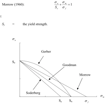
Mean stress effects in fatigue can be represented by constant-life diagrams, as shown in Figure 3.3. Stresses falling above the possible failure criteria lines result in failure. The most well known failure models are the Gerber line and the Modified Goodman line which are best used for fracture criteria, and the Soderberg line which is best used for yield criteria. The failure models are described by the following equations:
Gerber (1874): 1
2 = ⎟⎟ ⎠ ⎞ ⎜⎜ ⎝ ⎛ + u m e a S S σ σ
Morrow (1960): + =1 f m
e a
S σ
σ σ
Where:
Sy = the yield strength.
Figure 3.3 – Comparison of Constant Life Curves
Some general observations can be made on the failure criteria models when discussing cases of tensile mean stresses. The Gerber model is generally appropriate for ductile alloys but does not distinguish between tensile and compressive mean stresses. The Modified Goodman model is best suited for brittle metals. It is generally conservative for ductile alloys and it is generally non-conservative for compressive mean stresses. The Soderberg model is seldom used since this method is very conservative for most alloys.
Morrow
Soderberg
Goodman Gerber
m σ a
σ
f σ Se
Su
Sy
While the Basquin model, given by equation 3, is only valid for a mean stress of zero, a more general equation that accounts for a nonzero mean stress was developed by Morrow in 1968. This modified Basquin model is described by the following equation:
(
)( )
bf m f
a σ' σ 2N
σ = −
3.2.4 Modifying Factors
Several modifying factors are usually considered when using the stress-based approach for fatigue analysis of a smooth unnotched test specimen. Years of testing of the effects of various factors such as: surface finish and treatments (ka), size (kb), loading (kc),
temperature (kd), and other miscellaneous effects (ke) such as the environment have been
quantified as modification factors that result in a modified endurance limit often denoted as '
e
S . The modified endurance limit tends to be conservative with a correction for the remainder of the S-N curve not clearly defined. The modified endurance limit has the form:
e e d c b a
e k k k k k S S' =
The endurance limit will typically be reduced by the tensile mean stress, large section size, rough surface finish, chrome and nickel plating, decarburization (due to forging and hot rolling) and severe grinding. The endurance limit will typically be increased by modifying factors such as nitriding, carburization, shot peening, cold rolling, and induction hardening [31].
(8)
3.2.5 Notches
The discussion of the stress-based approach of fatigue has focused on nominally smooth-surfaced solid test specimens. However, almost all machine components and structural members invariably contain geometric or micro-structural discontinuities such as holes, fillets, grooves, and keyways. These discontinuities, or stress concentrations, cause the stress to be locally elevated, thus having a strong effect on how fatigue cracks nucleate and propagate [29].
The elastic stress concentration factor Kt relates the local stress ahead of the notch tip
to the far-field loading and is defined by the ratio of the maximum local stress at the discontinuity,
σ
max, to the nominal stress of the member, S.S Kt =σmax
This theoretical stress concentration factor is a function of the component geometry and loading and is available in many handbooks with the most popular and well used being that of Peterson [32].
Under fatigue loading conditions the effect of notches are accounted for by the fatigue notch factor Kf, which unlike Kt, is also dependent on material type.
( )
(notched)
e unnotched e f
S S K =
To account for these additional effects, the so-called notch sensitivity factor, q, was developed and is defined as
(10)
1 1 −
− =
t f K K
q
⎟⎟ ⎠ ⎞ ⎜⎜ ⎝ ⎛
+ =
ρ α 1
1 q
Where r is the notch-root radius and a is a constant dependent on the strength and ductility of the material. The parameter q varies from zero for no notch effect (Kf = 1) to unity for the
full effect predicted by elasticity theory (Kf = Kt).
3.2.6 Concluding Remarks
The S-N method is quite simple and can be used in almost any situation to obtain an initial rough estimate of the fatigue life. The method works well in applications of constant amplitude loading and designs involving long fatigue lives (effects due to variable amplitude loading will be discussed in a latter section). There are many existing S-N and test data readily available. However, this method is completely empirical and it derives from tensile tests of materials in the intermediate to long life region. Additionally, this method ignores plastic strains, which are critical for short fatigue lives, and this method is often dependent on geometry.
3.3 Strain-Life Approach
3.3.1 Introduction
The strain-life approach was initially developed independently by Coffin and Manson in the 1950’s. This method assumes that in many practical applications the engineering component response of the material will undergo plastic deformation, particularly at
yielding, which is often the case for low cycle fatigue (LCF) of ductile metals but may also be applied during high cycle fatigue (HCF) when there is little plasticity. Thus the strain-life approach differs significantly from the stress-life approach, as described earlier, which emphasizes nominal stresses and elastic stress concentration factors with empirical modifications.
Equivalent fatigue life (as well as fatigue damage which is discussed in Section 4.2) is assumed to occur in the material of an engineering component at the notch root and a smooth test specimen. This is due to the constraint imposed by the elastically stressed material surrounding the plastic zone when both are subjected to identical load histories as shown in Figure 3.4.
Figure 3.4 – Strain Based Approach for Fatigue of a Notched and Smooth Specimen
σ
S
σ
S
3.3.2 True Stress and Strain
A monotonic tensile test of a smooth cylindrical test specimen, which is obtained from a single load application, is typically used to determine the engineering stress and strain behavior of a material. However, in analyzing the results of tensile tests, the test specimen not only exhibits an increase in length but the specimen will also undergo a reduction in diameter. Therefore, the true stress is defined as the applied load P divided by the actual cross-sectional area A, rather than the original area Ao.
A P true = σ
Similarly, true strain is calculated from small increments in the instantaneous length and defined by
⎟⎟ ⎠ ⎞ ⎜⎜ ⎝ ⎛ =
o true
l l
ln
ε
It must be noted that the simple relationships given by Equations (13) and (14) are only valid up to necking. Once necking has occurred, the stress is not uniformly distributed across the section.
The difference between engineering and the true stress-strain response of a ductile material is shown in Figure 3.5. The true stress-strain curve consists of an elastic portion
( )
εe which is recovered when the load is removed and a plastic portion( )
εp which is notrecovered. They are both defined by the following relationships:
(13)
⎟ ⎠ ⎞ ⎜ ⎝ ⎛ =
E e
σ
ε p n
K
1
⎟ ⎠ ⎞ ⎜ ⎝ ⎛ = σ
ε
Where:
E = the elastic modulus
K = strain hardening coefficient
n = strain hardening exponent derived from monotonic stress-strain data. Ramberg and Osgood proposed that the total strain can be defined by the summation of the elastic and plastic strains.
Figure 3.5 – Comparison of Engineering and True Stress-Strain
3.3.3 Fatigue Life Relationships
If a test specimen is loaded in tension and then compression with yielding occurring at each load application of the half-cycle, the Bauschinger effect as seen in Figure 3.6 is
Engineering Strain, e
True Strain, ε
Engineering Stress,
S
True Stress,
σ
True σ-ε
Eng. S-ε
σf, εf
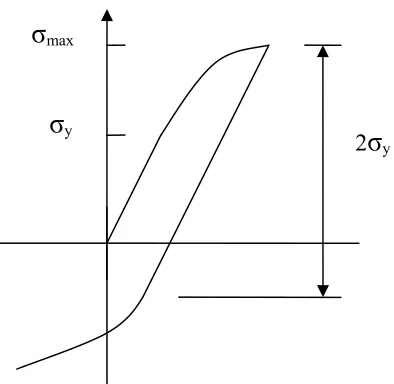
observed. If the test specimen is then loaded again in tension, completing one full cycle, the closed loop is known as a hysteresis loop as shown in Figure 3.7.
Figure 3.6 – Bauschinger Effect
Figure 3.7 – Hysteresis Loop 29 2
σ
yσ
maxCyclic stress-strain curves where a line from the origin passes through the tips of several loops, such as O-A-B-C in Figure 3.7 are used for assessing the durability of components and structures subjected to repeated loading, and are similar to monotonic stress-strain curves obtained during static load tests. The total width of loop C-H-F-G is Δε and the total height of the loop isΔσ, or total strain and stress ranges, respectively. The area within the loop represents a measure of the work done on the material due to plastic deformation. Thus, the total strain is the sum of the elastic and plastic strain ranges.
p e ε ε ε =Δ +Δ Δ
The response of a material subjected to a cyclic inelastic loading (that is at each load application yielding occurs) is in the form of a hysteresis loop and represents the true stress versus true strain and is defined by the following equation:
'
1
'
2
2 n
K
E ⎟⎠
⎞ ⎜ ⎝ ⎛ Δ + Δ =
Δε σ σ
Where primes are used to specify that the constants for the plastic term are from cyclic rather than monotonic stress-strain data and Δ represents the stress and strain ranges relative to coordinate axes at either loop tip. In addition, the stress-strain path for the hysteresis loops typically has the same shape as the cyclic stress-strain curve (Ramber-Osgood equation from cyclic stress-strain data) except for the addition of a scale factor of two.
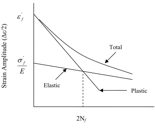
3.3.4 Strain-Life Curves
As with the stress-life approach, if several specimens are tested under different constant amplitude loads with a zero mean stress, test lives of the elastic and plastic regions
can be plotted on the basis of the true stress amplitude. By dividing both sides of Equation (3) (Basquin equation) by the elastic modulus E, the elastic strains commonly result in a linear relationship with a shallow slope when plotted on a log-log plot.
( )
bf f e N E E 2 2 2 ' σ σ ε = Δ = Δ
The Coffin-Manson equation showed that the relationship between plastic strain amplitude and endurance also commonly results in a linear relationship when plotted on a log-log plot, but with a much steeper slope.
( )
cf f p N 2 2 ' ε ε = Δ
Combining equations 18 and 19 results in the basis of the strain-life method, which relates the total strain amplitude to the fatigue life and is given by the following relationship [29]
( )
( )
43 42 1 43 42 1 plastic c f f elastic b ff N N
E 2 2
2 ' ' ε σ ε = + Δ Where: ' f
ε = the fatigue ductility coefficient
c = the fatigue ductility exponent
Figure 3.8 – Elastic, Plastic, and Total Strain vs. Life Curves
3.3.5 Mean Stress Effects
For the most part, the effect of mean strain is negligible on the fatigue life of a component. However, mean stress may have a significant effect on the fatigue life, predominantly at longer lives. Mean stress effects can either increase the fatigue life under compressive loads or decrease the fatigue life under tensile loads. A number of modifications to the strain-life equation, Equation (20), that incorporate the effect of mean stress are currently being used. However, no consensus exists on which approach is best [4].
Morrow suggested that the mean stress effect could be accounted for by modifying the elastic term in the strain-life equation by subtracting the mean stress, σm. The strain-live
equation then becomes
( )
( )
cf f b f m f N N E ' ' ' 2 2 2 ε σ σ ε + − = Δ Elastic Total Plastic ' f ε E f ' σ
Cycles to Failure (2Nf)
Another approach to account for mean stress effects was proposed by Smith, Watson, and Topper (SWT) [33]. They suggested that fatigue life was the product of strain amplitude and maximum stress in the cycle. Recalling Equation (3) at zero mean stress i.e. (σmax =
Δ
σ/2) and multiplying the strain-life equation by this term, results in
( ) ( )
( )
b cf f f b f f N N E + + = Δ 2 2 2 ' ' 2 2 '
max σ ε
σ σ
ε
3.3.6 Stress Concentrations
Stress concentration factors as described previously are equal to strain concentration factors when elastic deformation occurs at the tip of the notch. However, once the material yields at the notch tip (local yielding) the local stress
( )
σ and local strain( )
ε are no longer linearly related. Thus, concentration factors estimated by elastic analysis alone become invalid. At this point it becomes necessary to define separate stress and strain concentration factors, where S and e are the nominal stress and strain, respectively [29].S Kσ =σ
e Kε = ε
3.3.7 Nueber’s Rule
The strain-life method accounts for notch-root plasticity by requiring that the notch root stresses and strains be known. These are typically determined either experimentally by strain gage measurements or through numerical analysis such as finite elements. It is often advantageous to analyze an engineering component using linear elastic finite element
(22)
σ
ε
e eε σ σε =
σe, εe σ, ε
numerical analysis is sometimes necessary i.e. during fully plastic yielding, Neuber’s rule is a method used for estimating notch stresses and strains from a linear elastic model. Thus, it is essentially used as a correction factor. Neuber’s rule is defined by
ε
σK
K Kt =
This can be rearranged to directly convert stresses from an elastic finite element analysis (σe,
εe representing elastic stress-strain) into elastic-plastic stress-strain (σ, ε representing
elastic-plastic stress-strain). It is used with the cyclic and hysteresis stress-stain curves and the relationship can be seen in Figure 3.9.
Figure 3.9 – Neuber’s Rule
Assuming fully plastic yielding does not occur; Neuber’s rule for local yielding is defined by the following equation,
{
( )
3 2 1
load applied
t
response notch E
S K 2 = σε
(24)
3.3.8 Concluding Remarks
The strain-life method takes into account the actual stress-strain response of the material and thus accounts for localized plasticity. This method is suitable for estimating both long and short lives and it is well-suited for handling variable amplitude loading (discussed in Chapter 4). It can handle complicated geometries such as notches and it takes into account the mean stress correction. This method involves a relatively complicated analysis by hand but it is ideally suited with the use of computer analysis. The strain-life approach is attractive for practical reasons since strains can be measured using strain gages and it is well-suited for application with finite element analysis (FEA). However, this method along with the stress-based approach does not include an analysis of crack growth. The analysis of crack growth is accomplished through the use of fracture mechanics.
3.4 Fracture Mechanics Approach
3.4.1 Introduction
3.4.1.1 Linear Elastic Fracture Mechanics
In ductile materials, large plastic deformations occur in the vicinity of a crack tip since materials plastically deform as the yield stress is exceeded. As long as this region of plasticity remains small in relation to the overall dimensions of the crack and cracked body, the linear elastic fracture mechanics (LEFM) approach is valid. Thus the LEFM is a mature field in which the material is assumed to behave in a linear-elastic manner as defined by Hooke’s Law.
3.4.2 Loading Modes
A cracked body can be generally loaded in any one or a combination of the three modes of loading as shown in Figure 3.10. Mode I is the normal or opening mode, Mode II is the sliding or in-plane shear mode, and Mode III is the tearing or anti-plane shear mode. The following discussion deals with crack propagation due to Mode I since it is the most important for practical analysis within most engineering applications.
Figure 3.10 – Three Basic Independent Modes of Crack Deformation Mode
I
Mode II
3.4.3 Stress Intensity Factor
For a semi-infinite through-thickness crack of size a, in an infinite plate of an isotropic and homogeneous solid loaded in Mode I, the stress distribution near the crack tip is of the general form
( )
...2 +
= θ
π
θ I ij
ij f
r K
Where:
θij = the local stresses acting on an element dxdy at a distance r from the
crack tip and at an angle theta from the crack plane fij(θ) = known functions of theta
The stress intensity factor, KI where I denotes mode I loading, defines the magnitude of the
local stresses around the crack tip.
Figure 3.11 – Location of Local Stress near a Crack Tip
The stress intensity factor is affected by crack size and shape, loading, and geometry. For Mode I it has the general form,
txy
θ σy
σy
σ σ
r
a
σx σx
txy
Where:
σ = the applied far-field stress a = the crack length
F = a dimensionless correction factor that depends on geometry and loading
Solutions for stress intensity factors for a wide variety of problems have been obtained and published in several readily available handbooks [30].
3.4.4 Fracture Toughness
The value of the stress intensity factor, KI, at fracture is called the fracture toughness
and denoted Kc. Thus fracture occurs when KI equals Kc regardless of the shape of the body
or the size of the crack.
As discussed earlier, stresses are very high at the crack tip. Therefore, a large transverse strain should develop in the plastic zone. However, the material surrounding the plastic zone is at a much lower stress, which constrains the crack tip from contracting. This deters transverse strains from developing but the material is subjected to transverse stress. It must be noted that transverse stress will only develop if the material is sufficiently thick i.e. a plain strain condition. In a thin body, the out of plane stresses (σz) are zero equating to a plane stress condition [30].
toughness is called the plane strain fracture toughness and usually denoted KIc for mode I
loading.
3.4.5 Fatigue Crack Growth
It has been found that the majority of fatigue life occurs during the propagation of a crack. Therefore, fracture mechanics principles enable the prediction of the number of cycles for a crack to grow to some specified length or to final failure of the component.
Figure 3.12 – Idealized Regions of the Crack Growth Rate Curve
Crack growth behavior for constant amplitude loading can be described by the relationship between cyclic crack growth rate da/dN and the stress intensity range ΔK. Values of log da/dN versus values of log ΔK can be plotted for a given crack length as shown
III II
I
Kc ΔKth
ΔK
Log scale
the curve appears to approach a vertical asymptote in which the cracking behavior is associated with ΔKth called the fatigue crack growth threshold. It is in this region that crack
growth does not ordinarily occur. At higher growth rates, Region III, unstable crack growth occurs just prior to final failure. Most of the current applications of LEFM to describe crack growth occur in Region II. It is at these intermediate values of ΔK, that a straight line on a log-log plot is often observed. A relationship representing this line was developed by P. C. Paris in the early 1960’s and is given by
( )
mK C dN
da = Δ
Where:
C = material constant
m = material constant and slope of the log-log plot
ΔK = the stress intensity range Kmax - Kmin.
The crack growth life, in terms of cycles to failure under constant amplitude loading, may be calculated by integrating the Paris equation over the interval ai (the initial crack length) to af
(the final or critical crack length).
( )
∫
Δ= f i
a
a m
f
K C
da N
3.4.6 Mean Stress Effects
As with both the stress-life and strain-life approaches to fatigue, mean stresses can have a significant effect on the fatigue life of a component. An increase in the R-ratio of the cyclic loading causes growth rates for a given ΔK to be larger. Various empirical
(28)
relationships characterizing the effect of R on da/dN vs. ΔK curves will now briefly be discussed. One of the most widely used methods is based on applying the Walker relationship which is defined by the following equation
(
)
(
)
nm I R K C dN da − Δ = 1 Where:
n = material constant
Another proposed method to include R effects is that of Forman and is defined by the following equation.
( )
(
R)
K KK C dN da c m Δ − − Δ = 1
These models do not account for any micro-structural or environmental effects and need to be further modified.
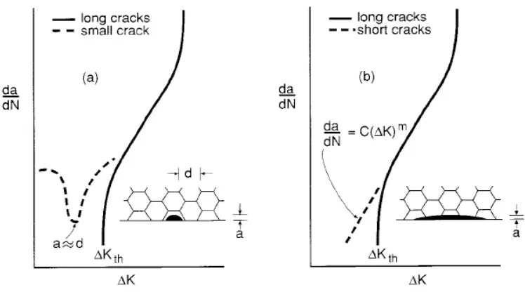
3.4.7 Crack Size Limitations
The practice of characterizing the growth of fatigue cracks on the basis of fracture mechanics typically relies on components containing long cracks or flaws with an initial length of about 0.05 inches [7]. However, if a crack is sufficiently small and thus interacts with the microstructure of the material it can have dramatic effects on crack growth behavior. The growth of small cracks, when described by LEFM, tends to grow faster than estimated from the usual da/dN vs. ΔK curves from test specimens with long cracks. This is illustrated
(30)
Figure 3.13 – Behavior of Small and Short Cracks on a Microstructural Scale 29
Small cracks are defined when all of its dimensions are comparable to the micro-structural dimensions, such as grain size, of the material. However, short cracks have one dimension that is large compared to the microstructure [29].
In the early 1970’s, Elber developed the theory of crack closure. He observed that the surfaces of fatigue cracks close as a result of crack-tip plasticity and thus cannot propagate until the applied stress exceeds the stress necessary to fully open the crack faces. Thus, from crack closure considerations, ΔK in Equation (28) is replaced by an effective stress intensity factor range, ΔKeff, which is smaller than ΔK and defined as
open eff K K
K = −
Δ max
(
S S)
aF( )
gKeff = − o π
Δ max
(32)
Where So is the crack-opening stress as calculated from the analytical closure model
developed by Newman9,14. To calculate the crack growth rate due to the effects of small cracks, Equation (28) becomes
(
)
( )
[
]
mo aF g S
S C dN
da = − π
max
Therefore, to calculate the total life of a component using the fracture mechanics approach a modified damage tolerance approach is used which incorporates the effects of small cracks. This approach is referred to as the total life analysis (TLA) and is described by Everett in reference [7].
3.4.8 Crack Propagation for Complex Components
Standard references are readily available giving values of the shape parameter or correction factor, F, of many simple classical shapes for use with the Paris, Walker, or Forman equations. However, in practice many components are of a complex shape and thus the fatigue crack growth equations with the shape parameter are not valid. This results in the need for a full FEA or boundary element analysis allowing for stress redistribution as the crack propagates. Another problem with complex components is defining the effective remote stress [4].
3.4.9 Concluding Remarks
The LEFM approach is the only method that deals directly with crack growth and provides a method to characterize the failure due to fracture. Crack growth rates can be
4 FATIGUE UNDER VARIABLE AMPLITUDE LOADING
Up to this point most of the discussion about fatigue has dealt with constant amplitude loading. Constant amplitude fatigue loading is defined as fatigue under cyclic loading with constant amplitude and a constant mean load. However, engineering components are usually subjected to variable amplitude loading which can be defined by complex loading histories of varying cyclic stress amplitudes, mean stresses and loading frequencies.
4.1 Cycle Counting
Time
St
ra
in
Figure 4.1 – Complex Load History
4.2 Cumulative Damage
As defined earlier, an engineering component’s total life can be separated into crack initiation and propagation stages. Thus, there are different approaches used in determining cumulative fatigue damage in regards to the safe-life and damage-tolerant approaches for fatigue.
4.3 Miner’s Rule
The linear cumulative damage hypothesis was first proposed by Palmgren36 as early as 1924 and further developed by Miner37 in 1945. This empirical damage summing method
for the initiation phase as determined by either the stress or strain life approach is best known as Miner’s Rule.
The load history as shown in Figure 4.2 consists of two blocks of constant amplitude loading, making up a variable amplitude load history. If the loading consists of only the largest cycle, Sa1, and it is assumed this load history will be repeated until failure, the
Figure 4.2 – Palmgren-Miner Rule for Life Prediction of a Variable Amplitude Loading 1 1 1 = N n Where:
n1 = the number of cycles at stress level Sa1
N1 = the number of cycles to failure as obtained from the fatigue life
endurance curve
The failure criterion for variable amplitude loading is simply the summation of the life fractions for each loading block, thus damage (Bf) is defined as
1 ... 1 3 3 2 2 1
1 + + + = =
=
∑
= m i i i f N n N n N n N n BAn alternative form of Miner’s rule has been proposed by Madayag38.
Where:
X = the desired factor of safety and is selected on the basis’s of the load history, usually less than 1
5 STANDARIZED LOAD SPECTRUM
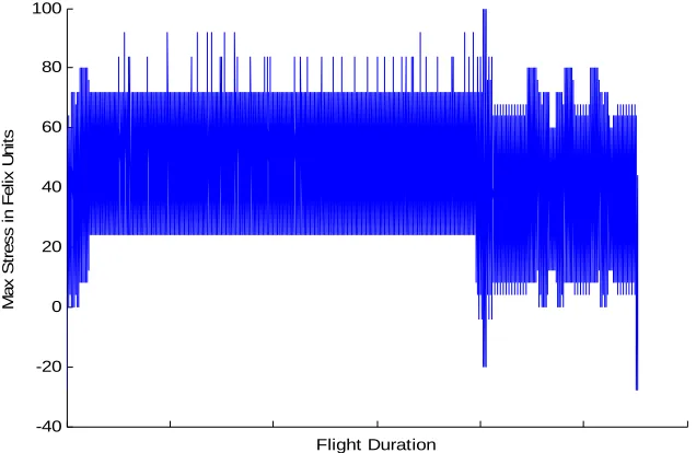
One of the more significant inputs in determining service life is the load spectrum [2]. The loading spectrum chosen for the validation portion of this work was that of a generalized helicopter loading sequence developed in a collaborative study by three European countries, which resulted in the development of two standardized spectra. The first is referred to as Helix and it is a loading sequence representative of hinged articulated rotors. The second spectrum, called Felix, is a loading sequence representative of fixed or semi-rigid rotors [39]. The load spectrum, Felix/28, is a shortened version of the Felix spectrum and consists of 161,034 cycles through one pass, while the full Felix sequence has over two million loading cycles through one pass.
The Felix spectrum is scaled in Felix units with a maximum load in the sequence being 100 units. The ground load at landing is -28 Felix units and all alternating loads below 16 Felix units were omitted. The Felix/28 spectrum was developed further by omitting all alternating loads below 28 Felix units.
-40 -20 0 20 40 60 80 100
Flight Duration
M
a
x
S
tr
e
s
s
in
F
e
lix
U
n
it
s
6 MULTIAXIAL FATIGUE 6.1 Introduction
The fatigue theories introduced thus far can only be applied under the conditions of uniaxial stress states. In many applications, engineering components experience biaxial states of stress as a result of combined loading due to bending and torsion. In this thesis, the discipline of multiaxial fatigue will only be introduced as it continues to be a topic of concentrated research. However, a general field of knowledge on multiaxial fatigue analysis methods is emerging [4].
Figure 6.1 – Test Specimen for Multiaxial Fatigue
6.2 Strain-Based Models
The three essential features of the strain-life methodology for fatigue consists of the stress-strain relationships, the stain-life relationship, and Neuber’s rule which is used as an elastic to elastic-plastic correction factor. Therefore, each of these must be extended in order to handle biaxial stress states in low cycle fatigue in which plasticity may occur.
If nodal stresses are biaxial and the direction of the principal stresses do not change during the load history, Neuber’s uniaxial elastic-plastic correction factor can be extended to the following relationship.
e ij e ij ij
ij ε σ ε σ +Δ =Δ Δ Δ
However, the complexity of this equation increases for cases where the principal stresses change direction.
separate. The application of the normal stress will cause the crack tip to experience the entire applied shear load by eliminating the friction between the mating faces [41].
Figure 6.2 – Shear and Tensile Load Applied at Crack Faces
Currently, one of the more widely used models for predicting crack initiation of ductile metals due to multiaxial loading is the Brown-Miller criterion. Brown and Miller extended Findley’s theory to incorporate strains. They proposed that the maximum fatigue damage occurs on the plane which experiences the maximum shear strain amplitude. The complete criterion is given by the following relationship [42]:
( )
( )
cf f b
f f
N N N
E 2 1.75 2
65 . 1 2 2
' '
max ε σ ε
γ
+ =
Δ + Δ
Where:
γmax = the maximum shear strain
ε
N = the strain normal to the plane which experiences the maximum shearstrain amplitude
σ, e γ
γ
σ, e
As discussed in Section 3.3.5, mean stress effects can have a significant impact on fatigue life. Thus, Morrow’s mean stress correction can be included in the Brown-Miller relationship. The constants 1.65 and 1.75 are derived based on the assumption that the Poisson ratios for elastic and plastic stresses are 0.3 and 0.5, respectively, and that cracks initiate on the plane of maximum shear strain. However, the values of these constants will change under complex variable amplitude loading due to the effects of the varying damaged plane, but the values shown here are almost universally accepted [4].
Other methods, such as the principal strain criterion is often used for the analysis of brittle metals. By replacing the axial strain in Equation (21) with the principal strain, a multiaxial fatigue criterion which only requires uniaxial materials data can be developed.
6.3 Critical Plane
Principal strains can change their orientation during multiaxial load histories, necessitating the use of a critical plane analysis. In these cases it is not always obvious which plane will experience the most severe strains because the phase relationship between stresses is not always constant when components are subjected to multiaxial loading. Critical plane methods resolve the strains onto a number of planes and calculate the damage on each plane. Therefore a successful model should be able to predict both the fatigue life and the dominant failure plane(s) [41]. Additionally, because of the different possible failure modes, no single damage model should be expected to be used universally.
Brown criterion [44], the Brown-Miller (developed with Kandil) criterion [42], and the more recent proposal by Chu, Conle and Bonnen [45].
7 FATIGUE ANALYSIS FROM FINITE ELEMENT METHODS
Finite element analysis (FEA), also called the finite element method (FEM), is a method of analyzing engineering components in which the geometry of the structure is discretized into a series of nodes and elements. Using this numerical technique, a solution in terms of stresses, strains, deflections, temperatures, and frequency response can be obtained. These results, in turn, can be used for fatigue analysis. Fatigue analysis software uses stress results from a linear elastic FE analysis.
Fatigue analysis from FEA models is a fairly new subject, and many of the analysis rules have yet to be established. However, since crack initiation predominately occurs on the surface of a component, nodal stresses are generally the preferred approach over integration point stresses and averaged elemental stresses [4, 6]. Additionally, life prediction is dependent on the accuracy of both the stress analysis and the fatigue damage analysis. Chu19,20 has stated that a 10% error in the stress calculation is likely to double the error in the calculation of fatigue damage. Therefore, careful attention must be given to geometry details, mesh density, load history, and material properties.
In a typical FE analysis, elements are joined at nodes, with each node having several values of stress calculated from adjacent elements. FE codes generally average these stresses, resulting in a single average nodal stress tensor for each node in the model. A good indication of the quality of the mesh is the difference between the averaged and un-averaged stresses at a node.
used primarily in the special case in which the nominal stress approaches the yield stress, in which an elastic-plastic FEA could be used [4].
To ensure that Miner’s Rule gives adequate life estimates for most engineering applications, fatigue analysis codes reduce the stress or strain amplitude at the endurance limit, which is determined from a constant amplitude test by 20% to 25%. This has become a common practice since under variable amplitude loading the endurance limit may disappear or its amplitude may be reduced [48].
Analyzing a linear elastic model with a single applied load history will consist of a finite element load case solution for the stresses at each node. The elastically calculated stress tensor for each node is multiplied by the load history to give a time history of the stress tensor. Fatigue software is used to calculate the time histories of the in-plane principal stresses and their corresponding directions at the surface of the model. The strain time history is then used in a strain life fatigue calculation and the process is repeated for each node in the model [4, 6].
to determine the most damaged plane at each node. Thus, the location of the most damaged node can be determined and it does not necessarily have to be located at the node of maximum stress.
Major advances have been made in fatigue analysis software over the past decade and the correlation between predicted fatigue life and fatigue life based on test results are improving. Software such as fe-safe and FE-Fatigue are able to predict hotspots and actual fatigue lives with relative accuracy and reasonable processing speed. This is accomplished using either the stress-life method or the strain-life method. Once the hotspots are determined the results can be exported back into a FEA code to determine crack propagation and fracture if necessary. The flow chart in Figure 7.1 outlines a FEA-based durability analysis procedure.
Figure 7.1 – Finite Element-Based Durability Analysis 6
Design
Fatigue Software FEA
ANSYS, I-DEAS ABAQUS, NASTRAN
Life Contours Redesign
Material Properties
Stress Results
8 COMPUTER SOFTWARE DESCRTIPTION AND VALIDATIONS 8.1 Fatigue Modeling Software Description
For this work, the commercially available software suite fe-safeWorks developed by Safe Technology Limited was used. Safe Technology is recognized as a world-wide leading supplier of durability software and consulting services. In particular, Safe Technology is the leader in multiaxial fatigue analysis solutions. Safe Technology was formed in 1987 as John Draper & Associates. The software suite has been used to optimize the design of an automotive suspension component for durability under multiaxial loading.
8.2 ANSYS Overview
Preprocessing is the first step for a fatigue analysis. The steps consist of creating the model and mesh and specifying the material properties, loads, and boundary conditions. Fe-safe can read FEA data (stresses, strains, and temperatures) from several other third-party software files. ANSYS [49] was chosen for its geometry modeling and high quality meshing capabilities along with the additional benefit that fatigue results can be post-processed directly in ANSYS.
8.3 FE-SAFE Overview